Download as PDF, PPTX

![Example 1: Learning for multi-armed bandit
problems
Multi-armed bandit problem: Let i ∈ {1, 2, . . . , K} be the K
arms of the bandit problem. νi is the reward distribution of arm
i and µi its expected value. T is the total number of plays. bt is
the arm played by the agent at round t and rt ∼ νbt
is the
reward it obtains.
Information: Ht = [b1, r1, b2, r2, . . . , bt , rt ] is a vector that
gathers all the information the agent has collected during the
first t plays. H the set of all possible histories of any length t.
Policy: The agent’s policy π : H → {1, 2, . . . , K} processes at
play t the information Ht−1 to select the arm bt ∈ {1, 2, . . . , K}:
bt = π(Ht−1).
8](https://image.slidesharecdn.com/ernst-inria-2011-talk-150328095645-conversion-gate01/75/Learning-for-exploration-exploitation-in-reinforcement-learning-The-dusk-of-the-small-formulas-reign-9-2048.jpg)
![Notion of regret: Let µ∗
= maxk µk be the expected reward of
the optimal arm. The regret of π is : Rπ
T = Tµ∗
−
T
t=1 rt . The
expected regret is E[Rπ
T ] =
K
k=1 E[Tk (T)](µ∗
− µk ) where
Tk (T) is the number of times the policy has drawn arm k on
the first T rounds.
Objective: Find a policy π∗
that for a given K minimizes the
expected regret, ideally for any T and any {νi}K
i=1 (equivalent to
maximizing the expected sum of rewards obtained).
Index-based policy: (i) During the first K plays, play
sequentially each arm (ii) For each t > K, compute for every
machine k the score index(Hk
t−1, t) where Hk
t−1 is the history of
rewards for machine k (iii) Play the arm with the largest score.
9](https://image.slidesharecdn.com/ernst-inria-2011-talk-150328095645-conversion-gate01/75/Learning-for-exploration-exploitation-in-reinforcement-learning-The-dusk-of-the-small-formulas-reign-10-2048.jpg)
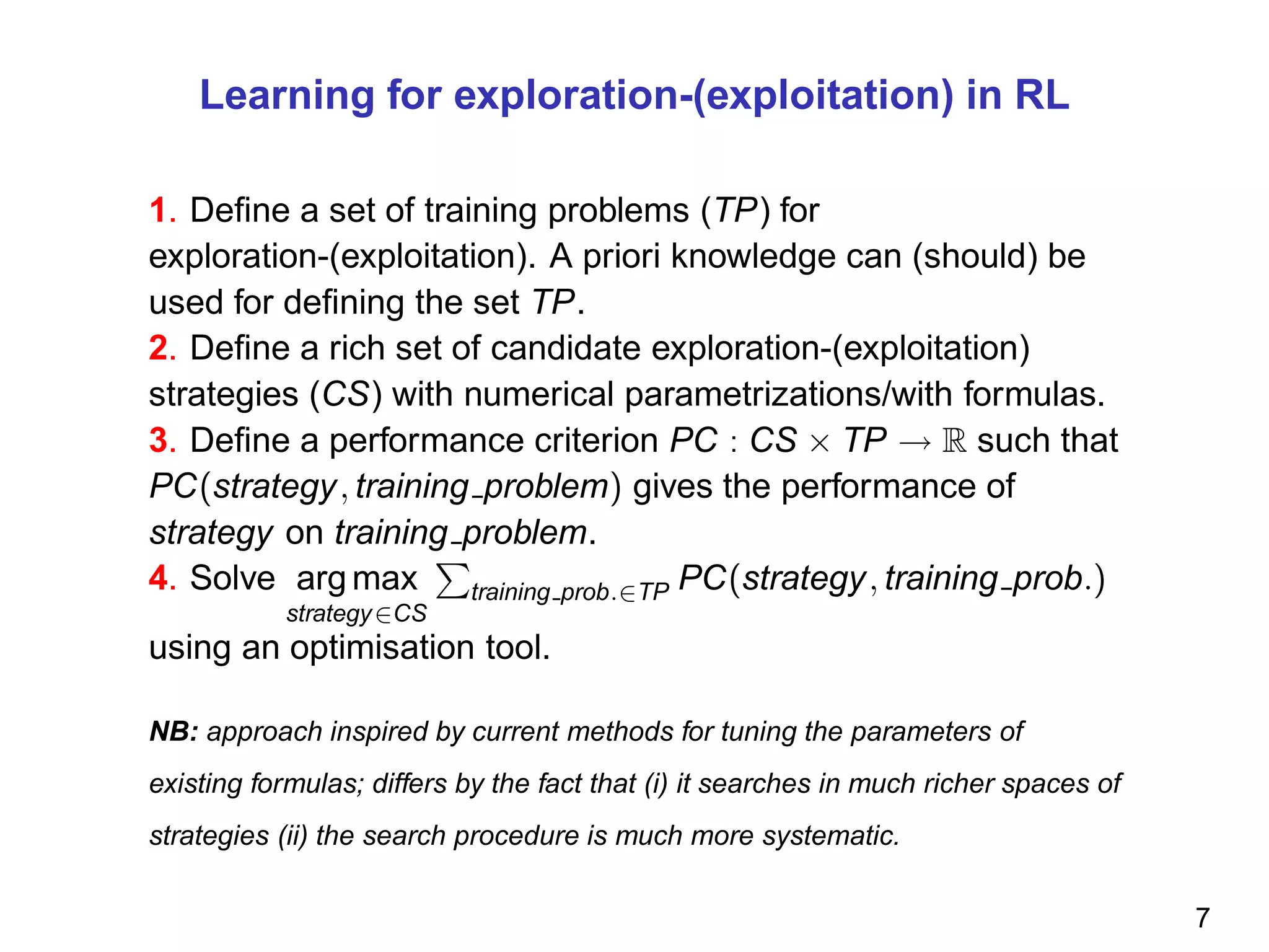
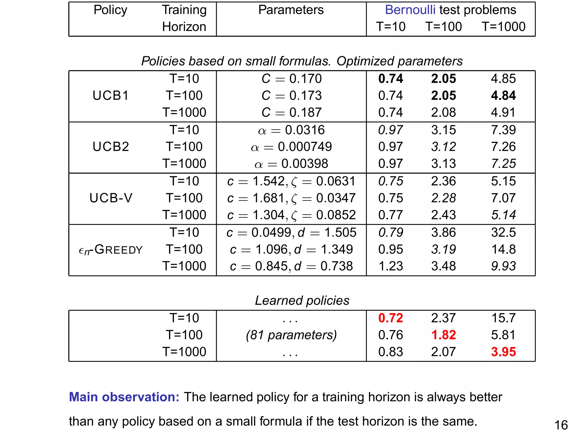
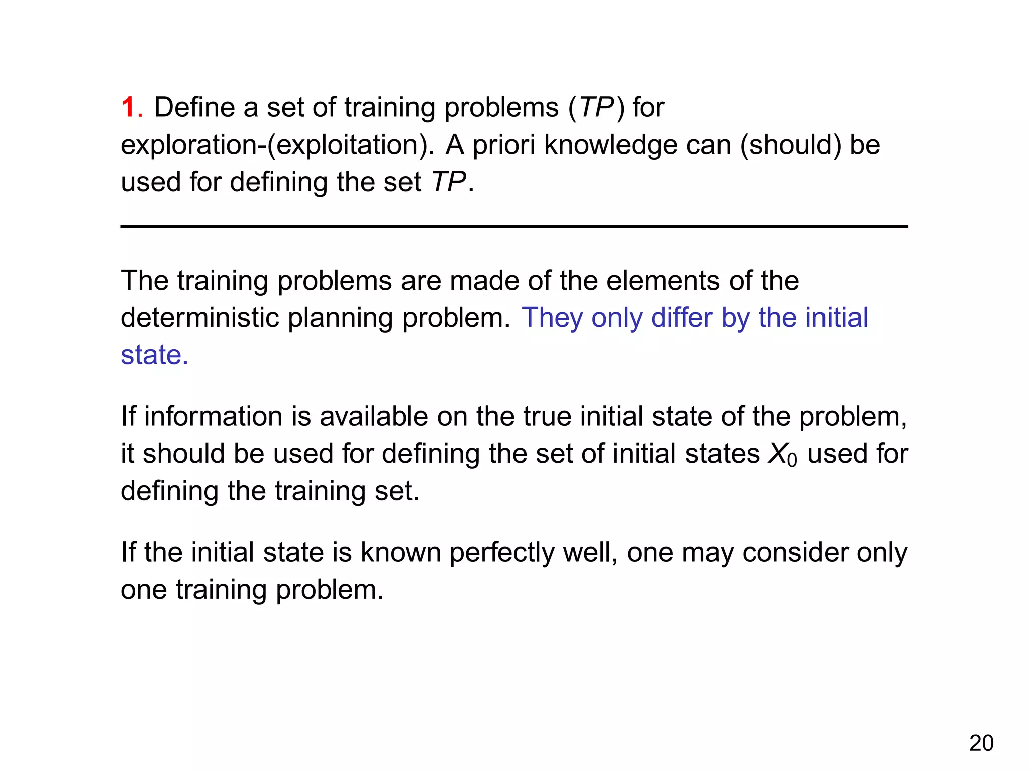
![1. Define a set of training problems (TP) for
exploration-exploitation. A priori knowledge can (should) be
used for defining the set TP.
In our simulations a training set is made of 100 bandit
problems with Bernouilli distributions, two arms and the same
horizon T. Every Bernouilli distribution is generated by
selecting at random in [0, 1] its expectation.
Three training sets generated, one for each value of the
training horizon T ∈ {10, 100, 1000}.
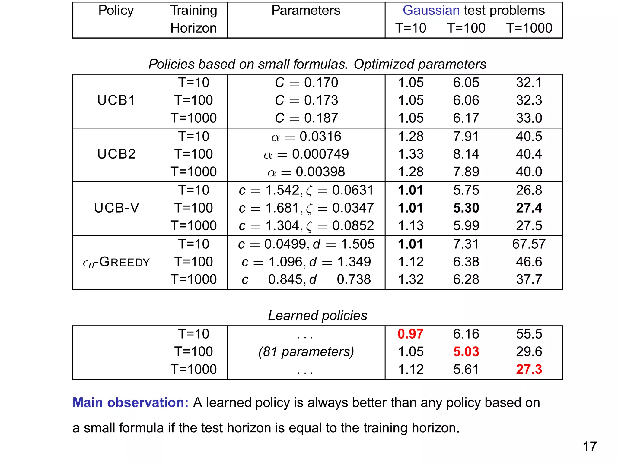
NB: In the spirit of supervised learning, the learned strategies are evaluated on
test problems different from the training problems. The first three test sets are
generated using the same procedure. The second three test sets are also
generated in a similar way but by considering truncated Gaussian distributions
in the interval [0, 1] for the rewards. The mean and the standard deviation of
the Gaussian distributions are selected at random in [0, 1]. The test sets count
10,000 elements.
10](https://image.slidesharecdn.com/ernst-inria-2011-talk-150328095645-conversion-gate01/75/Learning-for-exploration-exploitation-in-reinforcement-learning-The-dusk-of-the-small-formulas-reign-11-2048.jpg)
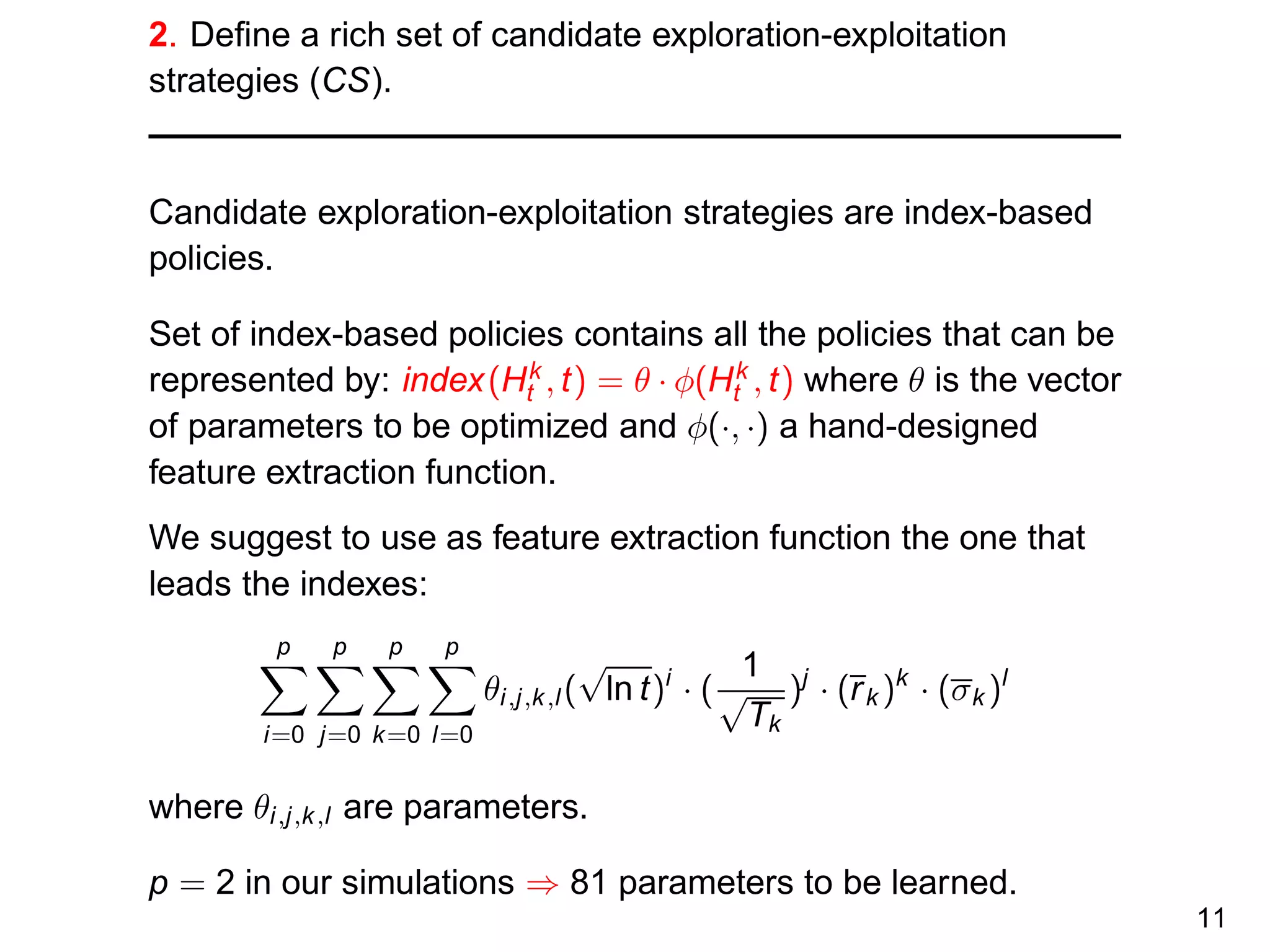


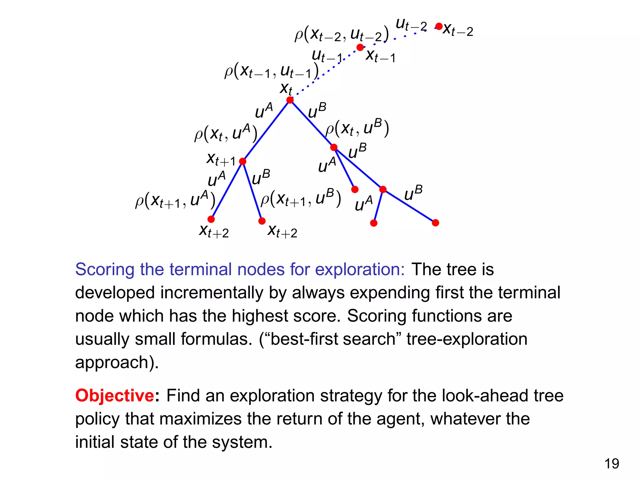
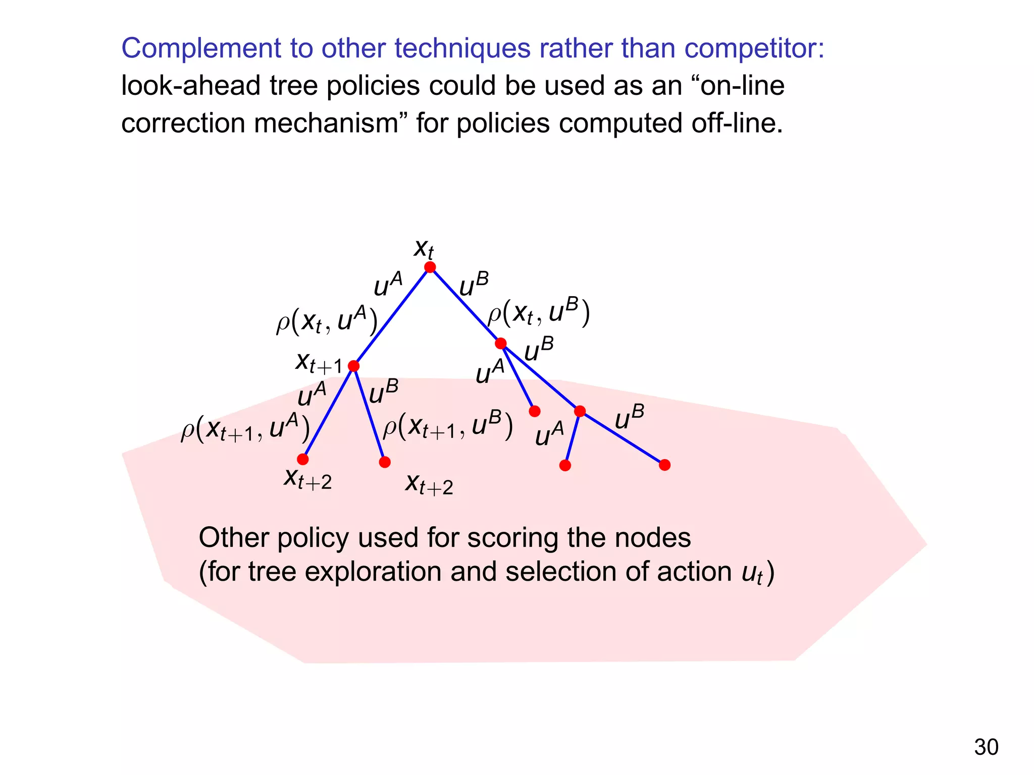
![2. Define a rich set of candidate exploration strategies (CS).
The candidate exploration strategies all grow the tree
incrementally, expending always the terminal node which has
the highest score according to a scoring function.
The set of scoring functions contain all the functions that take
as input a tree and a terminal node and that can be
represented by: θ · φ(tree, terminal node) where θ is the vector
of parameters to be optimized and φ(·, ·) a hand-designed
feature extraction function.
For problem where X ⊂ Rm
, we use as φ:
(x[1], . . . , x[m], dx[1], . . ., dx[m], rx[1], . . ., rx[m]) where x is the
state associated with the terminal node, d is its depth and r is
the reward collected before reaching this node.
21](https://image.slidesharecdn.com/ernst-inria-2011-talk-150328095645-conversion-gate01/75/Learning-for-exploration-exploitation-in-reinforcement-learning-The-dusk-of-the-small-formulas-reign-22-2048.jpg)
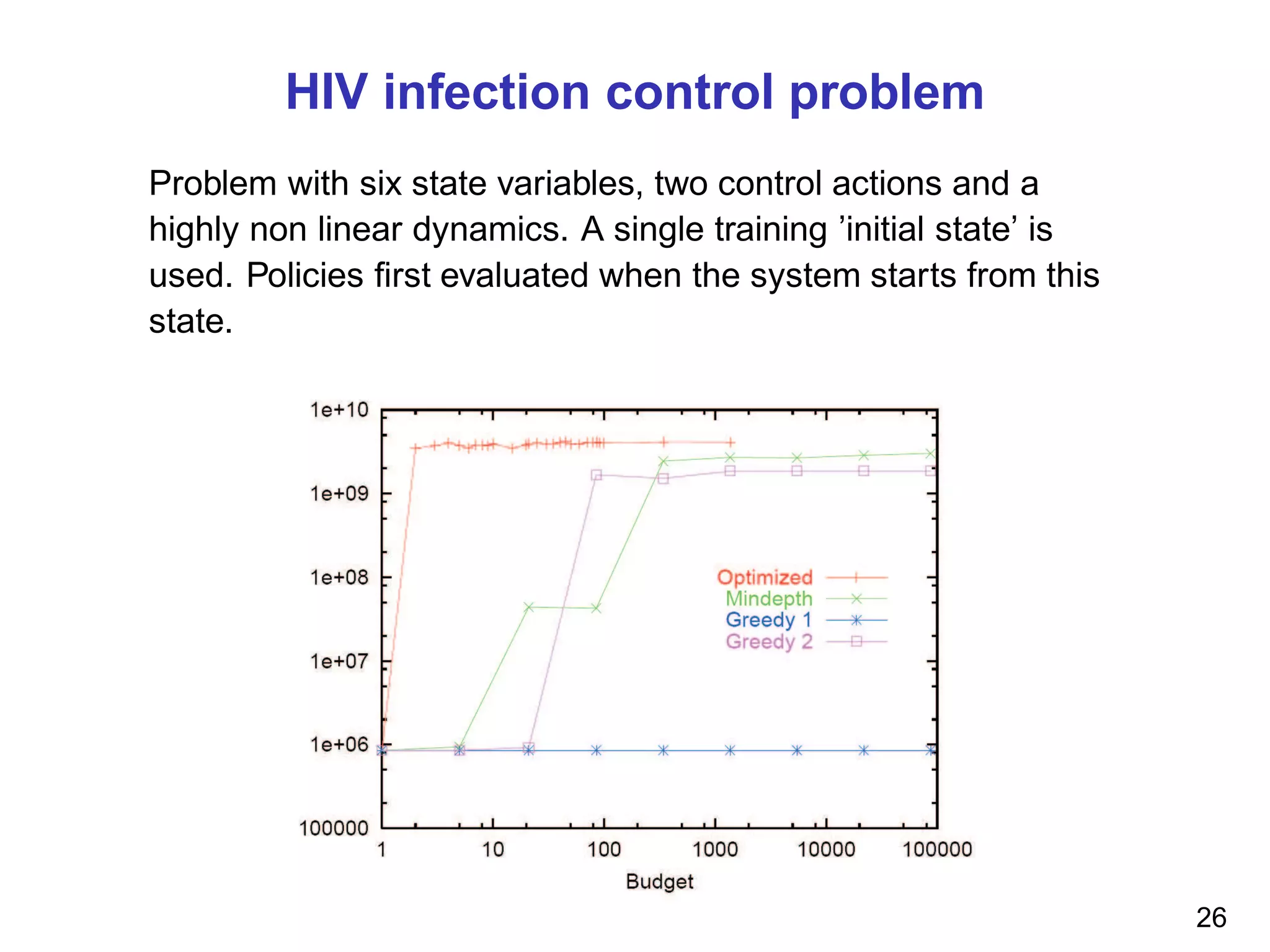
![2-dimensional test problem
Dynamics: (yt+1, vt+1) = (yt , vt ) + (vt , ut )0.1; X = R2
;
U = {−1, +1}; ρ((yt , vt ), ut ) = max(1 − y2
t+1, 0); γ = 0.9. The
initial states chosen at random in [−1, 1] × [−2, 2] for building
the training problems. Same states used for evaluation.
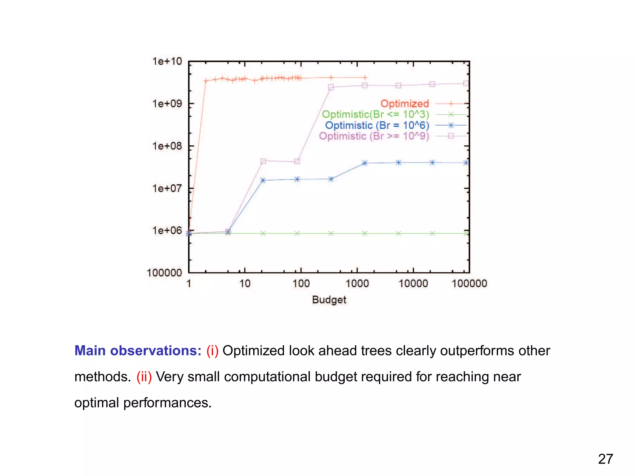
Main observation: (i) Optimized trees outperform other methods (ii) Small
computational budget needed for reaching near-optimal performances. 25](https://image.slidesharecdn.com/ernst-inria-2011-talk-150328095645-conversion-gate01/75/Learning-for-exploration-exploitation-in-reinforcement-learning-The-dusk-of-the-small-formulas-reign-26-2048.jpg)

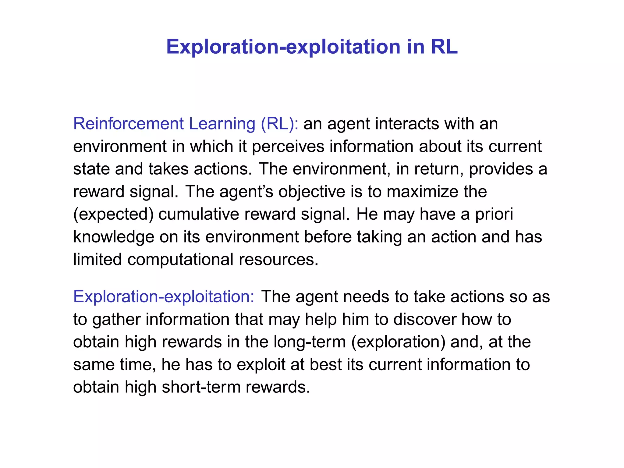
The document discusses reinforcement learning and the exploration-exploitation tradeoff that agents face. It proposes learning exploration-exploitation strategies rather than relying on predefined formulas. The approach defines training problems, candidate strategies parameterized by formulas, a performance criterion, and optimizes strategies on training problems using an estimation of distribution algorithm. Simulation results show learned strategies outperform strategies from common formulas on matching test problems.