Applications and Analysis of Bio-Inspired Eagle Strategy for 
Engineering Optimization 
Xin-She Yang and Mehmet Karamanoglu 
1 arXiv:1408.5320v1 [math.OC] 22 Aug 2014 
School of Science and Technology, Middlesex University, 
The Burroughs, London NW4 4BT, United Kingdom. 
T. O. Ting 
Department of Electrical and Electronic Engineering, 
Xi'an Jiaotong-Liverpool University, 
Suzhou, Jiangsu Province, P. R. China. 
Yu-Xin Zhao 
College of Automation, Harbin Engineering University, 
Harbin, P. R. China. 
Abstract 
All swarm-intelligence-based optimization algorithms use some stochastic components to 
increase the diversity of solutions during the search process. Such randomization is often repre- 
sented in terms of random walks. However, it is not yet clear why some randomization techniques 
(and thus why some algorithms) may perform better than others for a given set of problems. In 
this work, we analyze these randomization methods in the context of nature-inspired algorithms. 
We also use eagle strategy to provide basic observations and relate step sizes and search e- 
ciency using Markov theory. Then, we apply our analysis and observations to solve four design 
benchmarks, including the designs of a pressure vessel, a speed reducer, a PID controller and 
a heat exchanger. Our results demonstrate that eagle strategy with Levy 
ights can perform 
extremely well in reducing the overall computational eorts. 
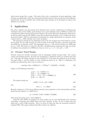
Citation details: X. S. Yang, M. Karamanoglu, T. O. Ting and Y. X. Zhao, Applications and 
Analysis of Bio-Inspired Eagle Strategy for Engineering Optimization Neural Computing and Appli- 
cations, vol. 25, No. 2, pp. 411-420 (2014). 
1 Introduction 
In contemporary neural computing, an active branch of research is the nature-inspired algorithms 
with diverse applications in engineering optimization. Most of these algorithms are based on the so- 
called swarm intelligence, and usually involve some form of non-deterministic, stochastic components, 
which often appear in terms of random walks. Such random walks can be surprisingly ecient when 
combined with deterministic components and elitism, as this has been demonstrated in many modern 
metaheuristic algorithms such as particle swarm optimization,
re
y algorithm and other algorithms 
[1, 18, 26, 29, 30, 32, 33, 34, 35]. 
Recent studies in nature-inspired algorithms have shown promising results with divers algorithms, 
including new algorithms such as accelerated particle swarm optimization [32, 11], bat algorithm [33], 
krill herd algorithm [10], 
ower algorithm [40], and other algorithms [35, 26]. A comprehensive review 
can be found in [5, 9, 38]. In all these algorithms, dierent degrees of randomization, exploration 
and exploitation have been used so as to maintain a good degree of solution diversity in the solution 
population, which helps to enhance the performance of these algorithms. Applications of modern 
nature-inspired algorithms have been very diverse with promising results [5, 6, 27, 12, 31].
In order to gain insight into the working mechanism of a stochastic algorithm, mathematical 
analysis of the key characteristics of random walks is necessary. Though there are some extensive 
studies of random walks with solid results in the statistical literature, most of these results are 
based on rigorous assumptions so as to obtain theoretical results using Markov chain models and/or 
Markov chain Monte Carlo methods [7, 8, 13, 14, 15, 29]. Consequently, such results may be too 
theoretical, and thus have not much practical implications for designing optimization algorithms. 
In addition, it is necessary to translate any relevant theoretical results in the right context so that 
they are truly useful to the optimization communities. The current work has extended our earlier 
work extensively [37]. Therefore, the aims of this paper are two-folds: to introduce the random 
walks and Levy 
ights in the proper context of metaheuristic optimization, and to use these results 
in the framework of Markov theory to analyze the iteration process of algorithms such as step sizes, 
eciency and the choice of some key parameters. 
The rest of the paper is organized as follows: Section 2 brie
y introduce the eagle strategy (ES). 
Section 3 introduces the fundamentals of random walks and discusses Levy 
ights, as well as their 
links to optimization via Markov chain theories. Section 4 analyzes the choice of step sizes, stopping 
criteria and eciency. Section 5 presents four case studies for engineering optimization applications. 
Finally, we brie
y draw the conclusions in Section 6. 
2 Eagle Strategy and Solution Diversity 
2.1 Eagle Strategy 
Eagle strategy developed by Xin-She Yang and Suash Deb [35] is a two-stage method for optimiza- 
tion. It uses a combination of crude global search and intensive local search employing dierent 
algorithms to suit dierent purposes. In essence, the strategy
rst explores the search space globally 
using a Levy 
ight random walk; if it
nds a promising solution, then an intensive local search 
is carried out by using a more ecient local optimizer such as hill-climbing and downhill simplex 
method. Then, the two-stage process starts again with new global exploration followed by a local 
search in a new region. The main steps of this method can be represented as the pseudo code as 
outlined in Fig. 1. 
The advantage of such a combination is to use a balanced tradeo between global search which 
is often slow and a fast local search. Some tradeo and balance are important. Another advantage 
of this method is that we can use any algorithms we like at dierent stages of the search or even at 
dierent stages of iterations. This makes it easy to combine the advantages of various algorithms so 
as to produce better results. 
It is worth pointing out that this is a methodology or strategy, not an algorithm. In fact, we 
can use dierent algorithms at dierent stages and at dierent time of the iterations. The algorithm 
used for the global exploration should have enough randomness so as to explore the search space 
diversely and eectively. This process is typically slow initially, and should speed up as the system 
converges, or no better solutions can be found after a certain number of iterations. On the other 
hand, the algorithm used for the intensive local exploitation should be an ecient local optimizer. 
The idea is to reach the local optimality as quickly as possible, with the minimal number of function 
evaluations. This stage should be fast and ecient. 
For the local optimizer in this paper, we will use the accelerated particle swarm optimization 
(APSO) [32] which is a simple but ecient variant of particle swarm optimization. The APSO 
essentially has one updating equation 
xt+1 
i = (1
)xti 
+
g + t; (1) 
where g is the current best solution among all the solutions xti 
at iteration t.
2 (0; 1) is a 
parameter, and  = O(1) is the scaling factor. Here t is a random number drawn from a standard 
normal distribution N(0; 1). As the typical scale L of a problem may vary,  should be linked to L 
as  = 0:1tL where t should decrease as the iterations proceed in the following form 
t = 0
t; (2) 
2
Objective function f(x) 
Initialization and random initial guess xt=0 
while (stop criterion) 
Global exploration by randomization (e.g. Levy 
ights) 
Evaluate the objectives and
nd a promising solution 
Intensive local search via an ecient local optimizer 
if (a better solution is found) 
Update the current best 
end 
Update t = t + 1 
end 
Figure 1: Pseudo code of the eagle strategy. 
where 0 2 (0:5; 1) and 0  
  1. From our previous parametric study, we will use 0 = 1,
= 0:5, 
and 
 = 0:97 [32]. 
2.2 Exploration, Exploitation and Solution Diversity 
In almost all nature-inspired algorithms, two con
icting and yet important components are explo- 
ration and exploitation, or diversi
cation and intensi
cation. The balance between these components 
are very important to ensure the good performance of an algorithm [1, 4]. In other words, a good 
degree of diversity should be maintained in the population of the solutions so that exploration and 
exploitation can be re
ected in the evolving population. If the population is too diverse, it is good 
for global exploration, but it may slow down the convergence. On the other hand, if the diversity 
is too low, intensive local exploitation may lead to premature convergence, and thus may loose the 
opportunity of
nding the global optimality. However, how to maintain good balance is still an 
unsolved problem, and dierent algorithms may have dierent ways of dealing with this issue. 
In most algorithms such as the particle swarm optimization, exploration and diversity can be 
considered as the steps by using random numbers, while intensi

Applications and Analysis of Bio-Inspired Eagle Strategy for Engineering Optimization

  • 1.
    Applications and Analysisof Bio-Inspired Eagle Strategy for Engineering Optimization Xin-She Yang and Mehmet Karamanoglu 1 arXiv:1408.5320v1 [math.OC] 22 Aug 2014 School of Science and Technology, Middlesex University, The Burroughs, London NW4 4BT, United Kingdom. T. O. Ting Department of Electrical and Electronic Engineering, Xi'an Jiaotong-Liverpool University, Suzhou, Jiangsu Province, P. R. China. Yu-Xin Zhao College of Automation, Harbin Engineering University, Harbin, P. R. China. Abstract All swarm-intelligence-based optimization algorithms use some stochastic components to increase the diversity of solutions during the search process. Such randomization is often repre- sented in terms of random walks. However, it is not yet clear why some randomization techniques (and thus why some algorithms) may perform better than others for a given set of problems. In this work, we analyze these randomization methods in the context of nature-inspired algorithms. We also use eagle strategy to provide basic observations and relate step sizes and search e- ciency using Markov theory. Then, we apply our analysis and observations to solve four design benchmarks, including the designs of a pressure vessel, a speed reducer, a PID controller and a heat exchanger. Our results demonstrate that eagle strategy with Levy ights can perform extremely well in reducing the overall computational eorts. Citation details: X. S. Yang, M. Karamanoglu, T. O. Ting and Y. X. Zhao, Applications and Analysis of Bio-Inspired Eagle Strategy for Engineering Optimization Neural Computing and Appli- cations, vol. 25, No. 2, pp. 411-420 (2014). 1 Introduction In contemporary neural computing, an active branch of research is the nature-inspired algorithms with diverse applications in engineering optimization. Most of these algorithms are based on the so- called swarm intelligence, and usually involve some form of non-deterministic, stochastic components, which often appear in terms of random walks. Such random walks can be surprisingly ecient when combined with deterministic components and elitism, as this has been demonstrated in many modern metaheuristic algorithms such as particle swarm optimization,
  • 2.
    re y algorithm andother algorithms [1, 18, 26, 29, 30, 32, 33, 34, 35]. Recent studies in nature-inspired algorithms have shown promising results with divers algorithms, including new algorithms such as accelerated particle swarm optimization [32, 11], bat algorithm [33], krill herd algorithm [10], ower algorithm [40], and other algorithms [35, 26]. A comprehensive review can be found in [5, 9, 38]. In all these algorithms, dierent degrees of randomization, exploration and exploitation have been used so as to maintain a good degree of solution diversity in the solution population, which helps to enhance the performance of these algorithms. Applications of modern nature-inspired algorithms have been very diverse with promising results [5, 6, 27, 12, 31].
  • 3.
    In order togain insight into the working mechanism of a stochastic algorithm, mathematical analysis of the key characteristics of random walks is necessary. Though there are some extensive studies of random walks with solid results in the statistical literature, most of these results are based on rigorous assumptions so as to obtain theoretical results using Markov chain models and/or Markov chain Monte Carlo methods [7, 8, 13, 14, 15, 29]. Consequently, such results may be too theoretical, and thus have not much practical implications for designing optimization algorithms. In addition, it is necessary to translate any relevant theoretical results in the right context so that they are truly useful to the optimization communities. The current work has extended our earlier work extensively [37]. Therefore, the aims of this paper are two-folds: to introduce the random walks and Levy ights in the proper context of metaheuristic optimization, and to use these results in the framework of Markov theory to analyze the iteration process of algorithms such as step sizes, eciency and the choice of some key parameters. The rest of the paper is organized as follows: Section 2 brie y introduce the eagle strategy (ES). Section 3 introduces the fundamentals of random walks and discusses Levy ights, as well as their links to optimization via Markov chain theories. Section 4 analyzes the choice of step sizes, stopping criteria and eciency. Section 5 presents four case studies for engineering optimization applications. Finally, we brie y draw the conclusions in Section 6. 2 Eagle Strategy and Solution Diversity 2.1 Eagle Strategy Eagle strategy developed by Xin-She Yang and Suash Deb [35] is a two-stage method for optimiza- tion. It uses a combination of crude global search and intensive local search employing dierent algorithms to suit dierent purposes. In essence, the strategy
  • 4.
    rst explores thesearch space globally using a Levy ight random walk; if it
  • 5.
    nds a promisingsolution, then an intensive local search is carried out by using a more ecient local optimizer such as hill-climbing and downhill simplex method. Then, the two-stage process starts again with new global exploration followed by a local search in a new region. The main steps of this method can be represented as the pseudo code as outlined in Fig. 1. The advantage of such a combination is to use a balanced tradeo between global search which is often slow and a fast local search. Some tradeo and balance are important. Another advantage of this method is that we can use any algorithms we like at dierent stages of the search or even at dierent stages of iterations. This makes it easy to combine the advantages of various algorithms so as to produce better results. It is worth pointing out that this is a methodology or strategy, not an algorithm. In fact, we can use dierent algorithms at dierent stages and at dierent time of the iterations. The algorithm used for the global exploration should have enough randomness so as to explore the search space diversely and eectively. This process is typically slow initially, and should speed up as the system converges, or no better solutions can be found after a certain number of iterations. On the other hand, the algorithm used for the intensive local exploitation should be an ecient local optimizer. The idea is to reach the local optimality as quickly as possible, with the minimal number of function evaluations. This stage should be fast and ecient. For the local optimizer in this paper, we will use the accelerated particle swarm optimization (APSO) [32] which is a simple but ecient variant of particle swarm optimization. The APSO essentially has one updating equation xt+1 i = (1
  • 6.
  • 7.
    g + t;(1) where g is the current best solution among all the solutions xti at iteration t.
  • 8.
    2 (0; 1)is a parameter, and = O(1) is the scaling factor. Here t is a random number drawn from a standard normal distribution N(0; 1). As the typical scale L of a problem may vary, should be linked to L as = 0:1tL where t should decrease as the iterations proceed in the following form t = 0 t; (2) 2
  • 9.
    Objective function f(x) Initialization and random initial guess xt=0 while (stop criterion) Global exploration by randomization (e.g. Levy ights) Evaluate the objectives and
  • 10.
    nd a promisingsolution Intensive local search via an ecient local optimizer if (a better solution is found) Update the current best end Update t = t + 1 end Figure 1: Pseudo code of the eagle strategy. where 0 2 (0:5; 1) and 0 1. From our previous parametric study, we will use 0 = 1,
  • 11.
    = 0:5, and = 0:97 [32]. 2.2 Exploration, Exploitation and Solution Diversity In almost all nature-inspired algorithms, two con icting and yet important components are explo- ration and exploitation, or diversi
  • 12.
  • 13.
    cation. The balancebetween these components are very important to ensure the good performance of an algorithm [1, 4]. In other words, a good degree of diversity should be maintained in the population of the solutions so that exploration and exploitation can be re ected in the evolving population. If the population is too diverse, it is good for global exploration, but it may slow down the convergence. On the other hand, if the diversity is too low, intensive local exploitation may lead to premature convergence, and thus may loose the opportunity of
  • 14.
    nding the globaloptimality. However, how to maintain good balance is still an unsolved problem, and dierent algorithms may have dierent ways of dealing with this issue. In most algorithms such as the particle swarm optimization, exploration and diversity can be considered as the steps by using random numbers, while intensi
  • 15.
    cation and exploitationare by the use of current global best. However, there is no direct control on how to switch between these components. Even in the accelerated particle swarm optimization (ASPO), diversity is mainly controlled by a random-walk-like term, while the control is indirectly carried out by an annealing- like reduction of randomness. On the other hand, eagle strategy provides a direct control of these two stages/steps in an iterative manner. First, solutions are sampled in a larger search space, and these solutions often have high diversity. These solutions are then fed into the APSO for evolution so that a converged state can be reached, and at the converged state, solution diversity is low. Then, a new set of samples are drawn again from the larger search space for another round of intensive APSO iteration stage. In this way, both exploration and exploitation have been used to main a good degree of diversity in the overall population, which also allows the system to converge periodically towards global optimality. As we will see in the late analysis of random walks and search strategies, randomization techniques are often used for exploration to increase the diversity of the solutions, while the selection of good solutions and evolution of an algorithm tend to lead to convergence of the system. However, their role is subtle. For example, in memetic algorithms, the balance is even more subtle [4]. It can be expected that the analysis in the rest of the paper can provide some insight into the working mechanisms and subtlety of random walks and randomization techniques in maintaining the good diversity of solutions in dierent algorithms. 3
  • 16.
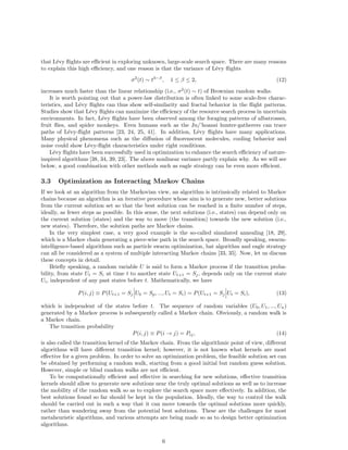
    3 Random Walksand Levy Flights as a Search Strategy In modern stochastic optimization algorithms, especially those based on swarm intelligence, there are often a deterministic component and a stochastic component, though traditional algorithms such as the steepest descent method are purely deterministic. Randomness is now an essential part of the stochastic search algorithms. Randomization techniques such as random walks have become an integrated part of a search process in stochastic algorithms. However, how to achieve the eective randomization remains an open question. The exact form of randomization may depend on the actual algorithm of interest. One of the objective of this paper is to analyze and discuss the main concepts of random walks and Levy ights, and their role in metaheuristic optimization. 3.1 Search via Random Walks In essence, a stochastic search process involves the use of a random process to generate new solutions in the search space so that the solutions can sample the landscape appropriately. However, the eectiveness of this sampling process depends on the random process used and the actual way of generating new solutions/samples. If the search space is treated as a black box (thus no knowledge or assumption about the modality is made), a random walk is one of the most simplest ways to carry out the search for optimality. Brie y speaking, a random walk is a random process which consists of taking a series of consecutive random steps [29, 34]. That is, the total moves SN after N steps are the sum of each consecutive random step Xi(i = 1; :::;N): SN = XN i=1 Xi = X1 + ::: + XN = NX1 i=1 Xi + XN = SN1 + XN; (3) where Xi is a random step drawn from a random distribution such as a normal distribution. De- pending on the perspective, the above relationship can also be considered as a recursive formula. That is, the next state SN will only depend on the current existing state SN1 and the move or transition XN from the existing state to the next state. In other words, the next state will depend only on the current state and the transition probability, and it has no direct link to the states in the past. From the Markov theory, we know that this is typically the main property of a Markov chain, to be introduced later. It is worth pointing out that there is no speci
  • 17.
    c restriction onthe step sizes. In fact, the step size or length in a random walk can be
  • 18.
    xed or varying.Random walks have many applications in physics, economics, statistics, computer sciences, environmental science and engineering. Mathematically speaking, a random walk can be de
  • 19.
    ned as St+1= St + wt; (4) where St is the current location or state at t, and wt is a step or random variable drawn from a known probability distribution. If each step or jump is carried out in the d-dimensional space, the random walk SN discussed earlier becomes a random walk in higher dimensions. In addition, there is no reason why the step length should be
  • 20.
    xed. In general,the step size can also vary according to a known distribution. If the step length obeys the Gaussian distribution, the random walk becomes the Brownian motion or a diusion process. As the number of steps N increases, the central limit theorem implies that the random walk should approach a Gaussian distribution. If the steps are drawn from a normal distribution with zero mean, the mean of particle locations is obviously zero. However, their variance will increase linearly with t. This is valid for the case without any drift velocity. In a more generalized case in the d-dimensional space, the variance of Brownian random walks can be written as 2(t) = jv0j2t2 + (2dD)t; (5) 4
  • 21.
    where v0 isthe drift velocity of the system [34, 41]. Here D = s2=(2 ) is the eective diusion coecient which is related to the step length s over a short time interval during each jump. For example, the well-known Brownian motion B(t) obeys a Gaussian distribution with zero mean and time-dependent variance: B(t) N(0; 2(t)); (6) where means the random variance obeys the distribution on the right-hand side; that is, samples should be drawn from the distribution. In physics and chemistry, a diusion process can be considered as a series of Brownian motion, which obeys the Gaussian distribution. Therefore, standard diusion is often referred to as the Gaussian diusion. If the motion at each step is not Gaussian, then the diusion is called non- Gaussian diusion. On the other hand, if the step lengths are drawn from other distributions, we have to deal with more generalized random walks. For example, a very special case is when step lengths obey the Levy distribution, such a random walk is called Levy ight or Levy walk [22, 41]. It is worth pointing out that a Levy ight is also a Markov chain. In fact, any algorithmic path traced by the current solution plus a transition probability forms a Markov chain. This is one of the reason why Markov chain theory can be used to analyzed stochastic algorithms such as simulated annealing and cuckoo search. In Section 4, we will discuss random walks without drift. That is, we will set v0 = 0. 3.2 Levy Flights In standard Gaussian random walks, the steps are drawn from a Gaussian normal distribution N(0; ), and these steps are mostly limited within 3. Therefore, it can be expected that very large steps ( 3) are extremely rarely. Sometimes, it may be necessary to generate new solutions that are far from the current state so as to avoid being trapped in a local region for a long time. In this case, random walks with varying step sizes may be desirable. For example, Levy ights are another class of random walks whose step lengths are drawn from the so-called Levy distribution. When steps are large, Levy distribution can be approximated as a simple power-law L(s) jsj1
  • 22.
  • 23.
    2 is anindex [16, 19, 21, 22]. However, this power-law is just an approximation to the Levy distribution. To be more accurate, Levy distribution should be de
  • 24.
    ned in termsof the following Fourier transform F(k) = exp[Ajkj
  • 25.
  • 26.
    2; (8) whereA is a scaling parameter. In general, the inverse of this integral is not straightforward, as no analytical form can be obtained, except for a few special cases. One special case
  • 27.
    = 2 corresponds to a Gaussian distribution, and another case
  • 28.
    = 1 leadsto a Cauchy distribution. Though the inverse integral is dicult, however, one useful technique is to approximate L(s) = 1 Z 1 0 cos(ks) exp[Ajkj
  • 29.
    ]dk; (9) whens is large. That is, L(s) ! A
  • 30.
  • 31.
  • 32.
  • 33.
    ; s !1; (10) where the Gamma function (z) is de
  • 34.
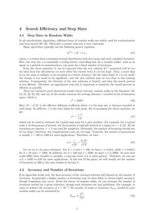
    ned as (z)= Z 1 0 tz1etdt: (11) Obviously, when z = n is an integer, it becomes (n) = (n 1)!. Since the steps drawn from a Levy distribution can be occasionally very large, random walks in terms of Levy ights are more ecient than standard Brownian random walks. It can be expected 5
  • 35.
    that Levy ightsare ecient in exploring unknown, large-scale search space. There are many reasons to explain this high eciency, and one reason is that the variance of Levy ights 2(t) t3
  • 36.
  • 37.
    2; (12) increasesmuch faster than the linear relationship (i.e., 2(t) t) of Brownian random walks. It is worth pointing out that a power-law distribution is often linked to some scale-free charac- teristics, and Levy ights can thus show self-similarity and fractal behavior in the ight patterns. Studies show that Levy ights can maximize the eciency of the resource search process in uncertain environments. In fact, Levy ights have been observed among the foraging patterns of albatrosses, fruit ies, and spider monkeys. Even humans such as the Ju/'hoansi hunter-gatherers can trace paths of Levy- ight patterns [23, 24, 25, 41]. In addition, Levy ights have many applications. Many physical phenomena such as the diusion of uorenscent molecules, cooling behavior and noise could show Levy- ight characteristics under right conditions. Levy ights have been successfully used in optimization to enhance the search eciency of nature- inspired algorithms [38, 34, 39, 23]. The above nonlinear variance partly explain why. As we will see below, a good combination with other methods such as eagle strategy can be even more ecient. 3.3 Optimization as Interacting Markov Chains If we look at an algorithm from the Markovian view, an algorithm is intrinsically related to Markov chains because an algorithm is an iterative procedure whose aim is to generate new, better solutions from the current solution set so that the best solution can be reached in a
  • 38.
    nite number ofsteps, ideally, as fewer steps as possible. In this sense, the next solutions (i.e., states) can depend only on the current solution (states) and the way to move (the transition) towards the new solution (i.e., new states). Therefore, the solution paths are Markov chains. In the very simplest case, a very good example is the so-called simulated annealing [18, 29], which is a Markov chain generating a piece-wise path in the search space. Broadly speaking, swarm- intelligence-based algorithms such as particle swarm optimization, bat algorithm and eagle strategy can all be considered as a system of multiple interacting Markov chains [33, 35]. Now, let us discuss these concepts in detail. Brie y speaking, a random variable U is said to form a Markov process if the transition proba- bility, from state Ut = Si at time t to another state Ut+1 = Sj , depends only on the current state Ui, independent of any past states before t. Mathematically, we have P(i; j) P(Ut+1 = Sj
  • 41.
    U0 = Sp;:::;Ut = Si) = P(Ut+1 = Sj
  • 44.
    Ut = Si);(13) which is independent of the states before t. The sequence of random variables (U0;U1; :::;Un) generated by a Markov process is subsequently called a Markov chain. Obviously, a random walk is a Markov chain. The transition probability P(i; j) P(i ! j) = Pij ; (14) is also called the transition kernel of the Markov chain. From the algorithmic point of view, dierent algorithms will have dierent transition kernel; however, it is not known what kernels are most eective for a given problem. In order to solve an optimization problem, the feasible solution set can be obtained by performing a random walk, starting from a good initial but random guess solution. However, simple or blind random walks are not ecient. To be computationally ecient and eective in searching for new solutions, eective transition kernels should allow to generate new solutions near the truly optimal solutions as well as to increase the mobility of the random walk so as to explore the search space more eectively. In addition, the best solutions found so far should be kept in the population. Ideally, the way to control the walk should be carried out in such a way that it can move towards the optimal solutions more quickly, rather than wandering away from the potential best solutions. These are the challenges for most metaheuristic algorithms, and various attempts are being made so as to design better optimization algorithms. 6
  • 45.
    4 Search Eciencyand Step Sizes 4.1 Step Sizes in Random Walks In all metaheuristic algorithms, dierent forms of random walks are widely used for randomization and local search [29, 33]. Obviously, a proper step size is very important. Many algorithms typically use the following generic equation: xt+1 = xt + s t; (15) where t is drawn from a standard normal distribution with zero mean and unity standard deviation. Here, the step size s is essentially a scaling factor, controlling how far a random walker, such as an agent or a particle in metaheursitics, can move for a
  • 46.
    xed number ofiterations. From the above equation, it can be expected that the new solution xt+1 generated will be too far away from the old solution (or more often the current best) if s is too large. Then, a move that is too far away is unlikely to be accepted as a better solution. On the other hand, if s is too small, the change is too small to be signi
  • 47.
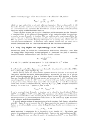
    cant, and thenew solution may be too close to the existing solution. Consequently, the diversity of the new solutions is limited, and thus the search process is not ecient. Therefore, an appropriate step size is important to maintain the search process as ecient as possible. There are extensive good theoretical results about isotropic random walks in the literature [16, 19, 21, 22, 24, 29], and one of the results concerns the average distance r traveled in the d-dimension space, which is r2 = 2dDt: (16) Here, D = s2=2 is the eective diusion coecient where s is the step size or distance traveled at each jump. In addition, is the time taken for each jump. By re-arranging the above equation, we get s2 = r2 t d ; (17) which can be used to estimate the typical step sizes for a give problem. For example, for a typical scale L of dimensions of interest, the local search is typically limited in a region of r = L=10. As the iterations are discrete, = 1 can used for simplicity. Obviously, the number of iterations should not be too large; otherwise, the computational costs are too high. Typically, the number of generations is usually t = 100 to 1000 for most applications. Therefore, we have s r p td = L=10 p t d : (18) Let us try to do some estimates. For d = 1 and t = 100, we have s 0:01L, while s 0:001L for d = 10 and t = 1000. In addition, for d = 100 and t = 1000, we have s L=3000. As step sizes could dier from variable to variable, a step size ratio s=L is more generic. Therefore, we can use s=L = 0:001 to 0:01 for most applications. In the rest of the paper, we will usually set the number of iterations as 200 in the case studies in Section 5. 4.2 Accuracy and Number of Iterations If an algorithm works well, the
  • 48.
    nal accuracy ofthe obtained solution will depend on the number of iterations. In principle, a higher number of iterations may be more likely to obtain higher accuracy, though stagnation may occur. From the theory of random walks, we can estimate the number of iterations needed for a given tolerance, though such estimates are just guidelines. For example, in order to achieve the accuracy of = 105, the number of steps or iterations Nmax needed by pure random walks can be estimated by Nmax L2 2d ; (19) 7
  • 49.
    which is essentiallyan upper bound. As an estimate for L = 10 and d = 100, we have Nmax 102 (105)2 100 1010; (20) which is a huge number that is not easily achievable in practice. However, this number is still far smaller than that needed by a uniform or brute force search method. It is worth pointing out the above estimate is the upper limit for the worst-case scenarios. In reality, most metaheuristic algorithms require far fewer numbers of iterations. Though the above estimate may be crude, it does imply another interesting fact that the number of iterations will not be aected much by dimensionality. In fact, higher-dimensional problems do not necessarily increase the number of iterations. This may lead to a rather surprising possibility that random walks may be ecient in higher dimensions if the optimization problem is highly multimodal. This may provide some hints for designing better algorithms by cleverly using random walks and other randomization techniques. As we will see below, dierent random walks will indeed lead to dierent convergence rates, and Levy ights are one of the best randomization techniques. 4.3 Why Levy Flights and Eagle Strategy are so Ecient As mentioned earlier, the variance of a Gaussian random walk increases linearly with time t, while the variance of Levy ights usually increases nonlinearly at a higher rate. As a result, if Levy ights instead of Gaussian random walks are used, the above estimate becomes Nmax L2 2d 1=(3
  • 50.
    ) : (21) If we use
  • 51.
    = 1:5 togetherthe same values of L = 10, d = 100 and = 105, we have Nmax 4:6 106: (22) It can be clearly seen that Levy ights can reduce the number of iterations by about 4 orders [O(104)] from O(1010) in Eq. (20) to O(106) in Eq. (22). Ideally, the step sizes in any nature-inspired algorithm should be controlled in such a way that they can do both local and global search more eciently. To illustrate this point, let us split the search process into two stages as those in the ecient Eagle Strategy (ES), developed by Xin-She Yang and Suash Deb [35, 36]. The
  • 52.
    rst stage usesa crude/large step, say, 1 = 102, and then in the second stage, a
  • 53.
    ner step size2 = 105 is used so as to achieve the same
  • 54.
    nal accuracy asdiscussed in the previous section. The
  • 55.
    rst stage cancover the whole region L1 = L, while the second region should cover smaller, local regions of size L2. Typically, L2 = O(L1=1000). Using the above values and L1 = L = 10 and L2 = L=1000 = 0:01, then we have N1;max 104; N2;max 104: (23) It can be seen clearly that the number of iterations can be reduced by about 6 orders (106) from O(1010) [see Eq. (20)] to O(104) [see Eq. (23)]. This approximate values for the number of iterations have been observed and used in the literature [38, 12]. For example, the typical number of iterations for bat algorithm in [12] and multiobjective cuckoo search in [38] are typically 20,000, which were indeed consistent with our estimations here. It is worth pointing out that the above reduction is by the two-stage Eagle Strategy only without using Levy ights. It can be expected that Levy ights can reduce the number of iterations even further. In fact, if Levy ights are used within the Eagle Strategy, then the above estimates can be reduced to N1;max N2;max 464; (24) which is obtained by substituting L1 (or L2) and 1 (or 2) into Eq. (21). The relative lower number of iterations can be both practical and realistic. Therefore, the good combination of Levy ights with Eagle Strategy can reduce the number of iterations from O(1010) to less than O(103), 8
  • 56.
    which works almostlike a magic. This shows that, with a combination of good algorithms, eagle strategy can signi
  • 57.
    cantly reduce thecomputational eorts and may thus increase the search eciency dramatically. It may be possible that a multi-stage eagle strategy can be developed to enhance this eciency even further. 5 Applications The above analyses and observations have indicated that a proper combination of randomization techniques such as Levy ights, eagle strategy and a good optimizer such as APSO can reduce the computational eorts dramatically and thus improve the search eciently signi
  • 58.
    cantly. Henceforth, wewill use eagle strategy with APSO to solve four nonlinear benchmarks so as to validate the above theoretical results. The four optimization benchmarks are: design optimization of a pressure vessel, a speed reducer, a PID controller and a heat exchanger. The parameter settings for the algorithms used in the rest of paper have been based on a para- metric study. For the eagle strategy, we used 5 rounds of two-stage iterations, and each round used the APSO for an intensive search. The population size is n = 20, and the iteration for APSO was set to t = 200. This leads to a total of 5 20 200 = 20; 000 function evaluations for each case study. In addition, the parameters in APSO have been set to be 0 = 1;
  • 59.
    = 0:5, and = 0:97. 5.1 Pressure Vessel Design Pressure vessels are literally everywhere such as champagne bottles and gas tanks. For a given volume and working pressure, the basic aim of designing a cylindrical vessel is to minimize the total cost. Typically, the design variables are the thickness d1 of the head, the thickness d2 of the body, the inner radius r, and the length L of the cylindrical section [2, 9]. This is a well-known test problem for optimization and it can be written as minimize f(x) = 0:6224d1rL + 1:7781d2r2 + 3:1661d21 L + 19:84d21 r; (25) subject to the following constraints: g1(x) = d1 + 0:0193r 0 g2(x) = d2 + 0:00954r 0 g3(x) = r2L 4 3 r3 + 1296000 0 g4(x) = L 240 0: (26) The simple bounds are 0:0625 d1; d2 99 0:0625; (27) and 10:0 r; L 200:0: (28) Recently, Cagnina et al [2] used an ecient particle swarm optimiser to solve this problem and they found the best solution f 6059:714 at x (0:8125; 0:4375; 42:0984; 176:6366): (29) This means the lowest price is about $6059:71. Using ES with APSO, we obtained the same results, but we used signi
  • 60.
    cantly fewer function evaluations, comparing with APSO alone and other methods. In fact, we use 5 stages and each stage with a total of 200 iterations. This is at least 10 times less than the iterations needed by standard PSO. This again con
  • 61.
    rmed that ESis indeed very ecient. 9
  • 62.
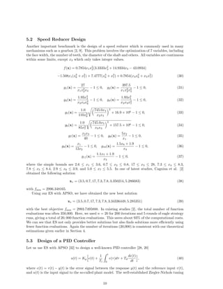
    5.2 Speed ReducerDesign Another important benchmark is the design of a speed reducer which is commonly used in many mechanisms such as a gearbox [2, 9]. This problem involves the optimization of 7 variables, including the face width, the number of teeth, the diameter of the shaft and others. All variables are continuous within some limits, except x3 which only takes integer values. f(x) = 0:7854x1x22 (3:3333x23 + 14:9334x3 43:0934) 1:508x1(x26 + x27 ) + 7:4777(x36 + x37 ) + 0:7854(x4x26 + x5x27 ) (30) g1(x) = 27 x1x22 x3 1 0; g2(x) = 397:5 x1x22 x23 1 0; (31) g3(x) = 1:93x34 x2x3x46 1 0; g4(x) = 1:93x35 x2x3x47 1 0; (32) g5(x) = 1:0 110x36 r745:0x4 x2x3 2 + 16:9 106 1 0; (33) g6(x) = 1:0 85x37 r745:0x5 x2x3 2 + 157:5 106 1 0; (34) g7(x) = x2x3 40 1 0; g8(x) = 5x2 x1 1 0; (35) g9(x) = x1 12x2 1 0; g10(x) = 1:5x6 + 1:9 x4 1 0; (36) g11(x) = 1:1x7 + 1:9 x5 1 0; (37) where the simple bounds are 2:6 x1 3:6, 0:7 x2 0:8, 17 x3 28, 7:3 x4 8:3, 7:8 x5 8:4, 2:9 x6 3:9, and 5:0 x7 5:5. In one of latest studies, Cagnina et al. [2] obtained the following solution x = (3:5; 0:7; 17; 7:3; 7:8; 3:350214; 5:286683) (38) with fmin = 2996:348165: Using our ES with APSO, we have obtained the new best solution x = (3:5; 0:7; 17; 7:3; 7:8; 3:34336449; 5:285351) (39) with the best objective fmin = 2993:7495888. In existing studies [2], the total number of function evaluations was often 350,000. Here, we used n = 20 for 200 iterations and 5 rounds of eagle strategy runs, giving a total of 20; 000 function evaluations. This saves about 93% of the computational costs. We can see that ES not only provides better solutions but also
  • 63.
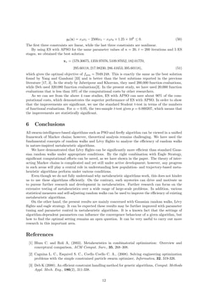
    nds solutions moreeciently using fewer function evaluations. Again the number of iterations (20,000) is consistent with our theoretical estimations given earlier in Section 4. 5.3 Design of a PID Controller Let us use ES with APSO [32] to design a well-known PID controller [28, 20] u(t) = Kp h e(t) + 1 Ti Z t 0 e( )d + Td de(t) dt i ; (40) where e(t) = r(t) y(t) is the error signal between the response y(t) and the reference input r(t), and u(t) is the input signal to the so-called plant model. The well-established Ziegler-Nichols tuning 10
  • 64.
    Figure 2: PIDcontroller design by ES with APSO. scheme can usually produce very good results. Here, we use ES with APSO to minimize the rise time, the overshoot and settling time. It is required to tune a third-order system with the following transfer function G(s) = 7 s3 + 3s2 + 3s + 1 ; (41) so that responses of the closed loop system to track a reference meet the following requirements: rise time is less than 1.5 s, settling time is less than 5.5 s, and the overshoot is less than 5%. If we use the standard Matlab control system toolbox [20], the obtained design by the Ziegler-Nichols scheme is GPID(s) = 0:311(1 + 1 2:3643s + 0:5911s); (42) which gives a rise time of 1.6 s, a settling time of 4.95, and overshoot of about 8.54%. Clearly, not all two requirements are met. In order to re
  • 65.
    ne the designs,we use ES with APSO, and the results are shown in Fig. 2. The
  • 66.
    nal design becomes 1 + GPID;new(s) = 0:5366 1 3:3940s + 0:8485s); (43) which gives a rise time of 1.0 s, a settling time of 5.25 s, and the overshoot of 4.97%. All the design requirements are met by this new design. As before, the total number of function evaluations is 20,000. 5.4 Heat Exchanger Design Heat transfer management is very important in many applications such as central heating systems and microelectronics. There are many well-known benchmarks for testing design/optimization tools, and one of the benchmarks is the design of a heat exchanger [33]. This design problem has 8 design variables and 6 inequality constraints, which can be written as Minimize f(x) = x1 + x2 + x3; (44) subject to g1(x) = 0:0025(x4 + x6) 1 0; (45) g2(x) = 0:0025(x5 + x7 x4) 1 0; (46) g3(x) = 0:01(x8 x5) 1 0; (47) g4(x) = 833:33252x4 + 100x1 x1x6 83333:333 0; (48) g5(x) = 1250x5 + x2(x4 x7) 120x4 0; (49) 11
  • 67.
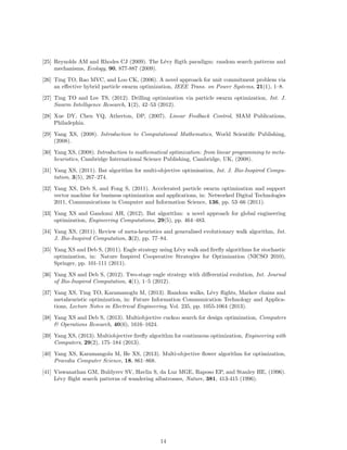
    g6(x) = x3x5 2500x5 x3x8 + 1:25 106 0: (50) The
  • 68.
    rst three constraintsare linear, while the last three constraints are nonlinear. By using ES with APSO for the same parameter values of n = 20, t = 200 iterations and 5 ES stages, we obtained the best solution x = (579:30675; 1359:97076; 5109:97052; 182:01770; 295:60118; 217:98230; 286:41653; 395:60118); (51) which gives the optimal objective of fmin = 7049:248. This is exactly the same as the best solution found by Yang and Gandomi [33] and is better than the best solutions reported in the previous literature [17, 3]. In the study by Jaberipour and Khorram, they used 200,000 function evaluations, while Deb used 320,080 function evaluations[3]. In the present study, we have used 20,000 function evaluations that is less than 10% of the computational costs by other researchers. As we can see from the above 4 case studies, ES with APSO can save about 90% of the com- putational costs, which demonstrates the superior performance of ES with APSO. In order to show that the improvements are signi
  • 69.
    cant, we usethe standard Student t-test in terms of the numbers of functional evaluations. For = 0:05, the two-sample t-test gives p = 0:000207, which means that the improvements are statistically signi
  • 70.
    cant. 6 Conclusions All swarm-intelligence-based algorithms such as PSO and
  • 71.
    re y algorithm canbe viewed in a uni
  • 72.
    ed framework ofMarkov chains; however, theoretical analysis remains challenging. We have used the fundamental concepts of random walks and Levy ights to analyze the eciency of random walks in nature-inspired metaheuristic algorithms. We have demonstrated that Levy ights can be signi
  • 73.
    cantly more ecientthan standard Gaus- sian random walks under appropriate conditions. By the right combination with Eagle Strategy, signi
  • 74.
    cant computational eortscan be saved, as we have shown in the paper. The theory of inter- acting Markov chains is complicated and yet still under active development; however, any progress in such areas will play a central role in understanding how population- and trajectory-based meta- heuristic algorithms perform under various conditions. Even though we do not fully understand why metaheuristic algorithms work, this does not hinder us to use these algorithms eciently. On the contrary, such mysteries can drive and motivate us to pursue further research and development in metaheuristics. Further research can focus on the extensive testing of metaheuristics over a wide range of large-scale problems. In addition, various statistical measures and self-adjusting random walks can be used to improve the eciency of existing metaheuristic algorithms. On the other hand, the present results are mainly concerned with Gaussian random walks, Levy ights and eagle strategy. It can be expected these results may be further improved with parameter tuning and parameter control in metaheuristic algorithms. It is a known fact that the settings of algorithm-dependent parameters can in uence the convergence behaviour of a given algorithm, but how to
  • 75.
    nd the optimalsetting remains an open question. It can be very useful to carry out more research in this important area. References [1] Blum C. and Roli A, (2003). Metaheuristics in combinatorial optimization: Overview and conceptural comparison, ACM Comput. Surv., 35, 268{308. [2] Cagnina L. C., Esquivel S. C., Coello Coello C. A., (2008). Solving engineering optimization problems with the simple constrained particle swarm optimizer, Informatica, 32, 319-326. [3] Deb K (2000). An ecient constraint handling method for genetic algorithms, Comput. Methods Appl. Mech. Eng., 186(2), 311-338. 12
  • 76.
    [4] Ferrante N.,(2012). Diversity management in memetic algorithms, in: Handbook of Memetic Algorithms, Studies in Computational Intelligence, Springer Berlin, vol. 379, pp. 153{165. [5] Fister I., Fister Jr I., Yang X. S., Brest J., (2013). A comprehensive review of
  • 77.
    re y algorithms, Swarmand Evolutionary Computation, (in press) DOI 10.1016/j.swevo.2013.06.001. [6] Fister I., Yang X. S., Brest J., Fister Jr. I., (2013). Modi
  • 78.
  • 79.
    re y algorithm usingquaternion representation, Expert Systems with Applications, 40(16), 7220{7230. [7] Fishman GS, (1995). Monte Carlo: Concepts, Algorithms and Applications, Springer, New York, (1995). [8] D. Gamerman, Markov Chain Monte Carlo, Chapman Hall/CRC, (1997). [9] Gandomi A. H., Yang X. S., and Alavi A. H., (2013). Cuckoo search algorithm: a metaheuristic approach to solve structural optimization problems, Engineering with Computers, 29(1), 17{35. [10] Gandomi A. H., and Alavi A. H., (2012). Krill herd: a new bio-inspired optimization algorithm, Communications in Nonlinear Science and Numerical Simulation, 17(12), pp. 4831{4845. [11] Gandomi A. H., Yun G. J., Yang X. S., Talatahari S., (2013). Chaos-enhanced accelerated particle swarm optimization, Communications in Nonlinear Science and Numerical Simulation, 18(2), 327{340. [12] Gandomi A. H., Yang X. S., Alavi A. H., Talatahari S., (2013). Bat algoritm for constrained optimization tasks, Neural Computing and Applications, 22(6), 1239{1255. [13] Geyer CJ, (1992). Practical Markov Chain Monte Carlo, Statistical Science, 7, 473{511. [14] Ghate A. and Smith R., (2008). Adaptive search with stochastic acceptance probabilities for global optimization, Operations Research Lett., 36, 285{290. [15] Gilks WR,Richardson S, and Spiegelhalter DJ, (1996). Markov Chain Monte Carlo in Practice, Chapman Hall/CRC. [16] Gutowski M., (2001). Levy ights as an underlying mechanism for global optimization algo- rithms, ArXiv Mathematical Physics e-Prints, June, (2001). [17] Jaberipour M and Khorram E, (2010). Two improved harmony search algorithms for solving engineering optimization problems, Commun. Nonlinear Sci. Numer. Simulat., 15 (11), 3316- 31 (2010). [18] Kirkpatrick S, Gellat CD and Vecchi MP, (1983). Optimization by simulated annealing, Science, 220, 670{680. [19] Mantegna RN, (1994). Fast, accurate algorithm for numerical simulation of Levy stable stochas- tic processes, Physical Review E, 49, 4677{4683. [20] Matlab R , Control System Toolbox, R2012a, version 7.14, (2012). [21] Nolan JP, (2009). Stable distributions: models for heavy-tailed data, American University. [22] Pavlyukevich I, (2007). Levy ights, non-local search and simulated annealing, J. Computa- tional Physics, 226, 1830{1844. [23] Ramos-Fernandez G, Mateos JL, Miramontes O, Cocho G, Larralde H, Ayala-Orozco B, (2004). Levy walk patterns in the foraging movements of spider monkeys (Ateles georoyi),Behav. Ecol. Sociobiol., 55, 223-230. [24] Reynolds AM and Frye MA, (2007). Free- ight odor tracking in Drosophila is consistent with an optimal intermittent scale-free search, PLoS One, 2, e354 (2007). 13
  • 80.
    [25] Reynolds AMand Rhodes CJ (2009). The Levy igth paradigm: random search patterns and mechanisms, Ecology, 90, 877-887 (2009). [26] Ting TO, Rao MVC, and Loo CK, (2006). A novel approach for unit commitment problem via an eective hybrid particle swarm optimization, IEEE Trans. on Power Systems, 21(1), 1{8. [27] Ting TO and Lee TS, (2012). Drilling optimization via particle swarm optimization, Int. J. Swarm Intelligence Research, 1(2), 42{53 (2012). [28] Xue DY, Chen YQ, Atherton, DP, (2007). Linear Feedback Control, SIAM Publications, Philadephia. [29] Yang XS, (2008). Introduction to Computational Mathematics, World Scienti
  • 81.
    c Publishing, (2008). [30] Yang XS, (2008). Introduction to mathematical optimization: from linear programming to meta- heuristics, Cambridge International Science Publishing, Cambridge, UK, (2008). [31] Yang XS, (2011). Bat algorithm for multi-objective optimisation, Int. J. Bio-Inspired Compu- tation, 3(5), 267{274. [32] Yang XS, Deb S, and Fong S, (2011). Accelerated particle swarm optimization and support vector machine for business optimization and applications, in: Networked Digital Technologies 2011, Communications in Computer and Information Science, 136, pp. 53{66 (2011). [33] Yang XS and Gandomi AH, (2012). Bat algorithm: a novel approach for global engineering optimization, Engineering Computations, 29(5), pp. 464{483. [34] Yang XS, (2011). Review of meta-heuristics and generalised evolutionary walk algorithm, Int. J. Bio-Inspired Computation, 3(2), pp. 77{84. [35] Yang XS and Deb S, (2011). Eagle strategy using Levy walk and
  • 82.
    re y algorithms forstochastic optimization, in: Nature Inspired Cooperative Strategies for Optimization (NICSO 2010), Springer, pp. 101-111 (2011). [36] Yang XS and Deb S, (2012). Two-stage eagle strategy with dierential evolution, Int. Journal of Bio-Inspired Computation, 4(1), 1{5 (2012). [37] Yang XS, Ting TO, Karamanoglu M, (2013). Random walks, Levy ights, Markov chains and metaheuristic optimization, in: Future Information Communication Technology and Applica- tions, Lecture Notes in Electrical Engineering, Vol. 235, pp. 1055-1064 (2013). [38] Yang XS and Deb S, (2013). Multiobjective cuckoo search for design optimization, Computers Operations Research, 40(6), 1616{1624. [39] Yang XS, (2013). Multiobjective
  • 83.
    re y algorithm forcontinuous optimization, Engineering with Computers, 29(2), 175{184 (2013). [40] Yang XS, Karamangolu M, He XS, (2013). Multi-objective ower algorithm for optimization, Procedia Computer Science, 18, 861{868. [41] Viswanathan GM, Buldyrev SV, Havlin S, da Luz MGE, Raposo EP, and Stanley HE, (1996). Levy ight search patterns of wandering albatrosses, Nature, 381, 413-415 (1996). 14