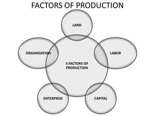
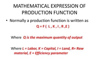
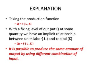
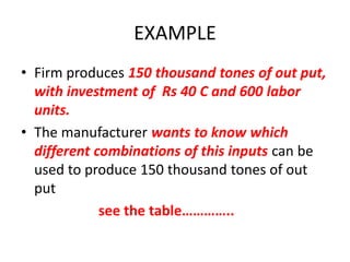
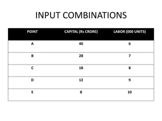
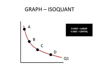
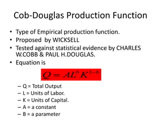
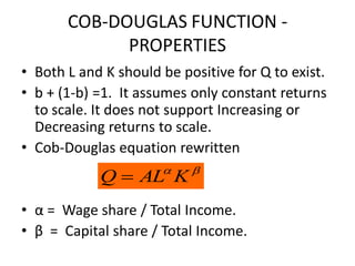
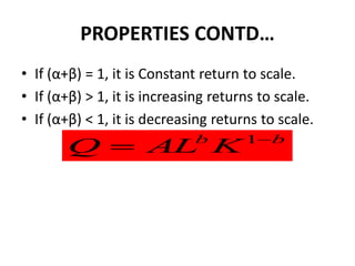
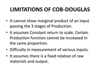
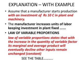
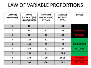
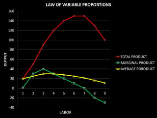
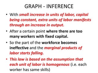
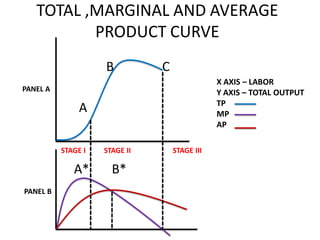
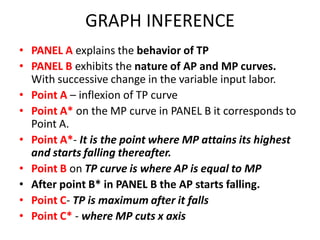
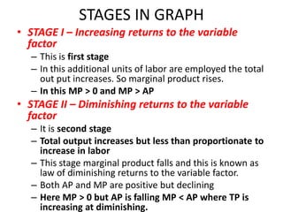
1. The document discusses production and costs faced by firms. It defines production and the different types of inputs used, including fixed and variable inputs. 2. It explains the concept of production functions, which show the maximum output achievable from different input combinations. Production functions can have one or two variable inputs, corresponding to short and long run analyses. 3. The law of variable proportions is described, where marginal and average product initially increase with more of a variable input but eventually diminish, leading to stages of increasing, diminishing, and negative returns. Graphs demonstrate these relationships between total, marginal, and average product curves.

1. PRODUCTION AND COST

2. INTRODUCTION
• Up to this you have learnt all about demand,
consumers , their preferences and decision
making.
• Now we would learn about producers
preference and their behavior though the
concept of optimum production with efficient
choice of differ factor inputs.

3. ….contd
• The basic problem that any firm faces is
duality of paradoxical objectives
– Maximum output.
– Minimum cost.
• In the next sessions we are going to discuss
how can a firm achieve this objective.
• What are the resources they may use, how to
combine them , what are the constraints in
optimization of production etc

4. PRODUCTION
• Production is the process of transformation
of inputs into goods and services of utility to
consumers and /or producers.
• It is a process of creation of value or wealth
through the production of goods and services
that have economic value to either
consumers or other producers.
• The process of adding value may occur
– By change in form(input to out put)
– Change in place(factory to retailer)
– By change in hands(retailer to consumer)

5. TYPES OF INPUTS
• You know what is production……………..?
• What are the inputs…………….?
• What are their characteristics…………….?
• Let us start with technology
– Technology is one of the most important input in any
of production process.
– Technology determines the type, quantity and
proportion of inputs
– It determines the maximum limit of output from a
given combination of inputs.

6. FIXED AND VARIABLE INPUTS
• Typically the production analysis of a firm is
done using two distinct time frames
– Short run production
• Period of time when the firm cannot vary some of its
inputs
• Supply of some inputs are fixed
– Long run production
• Have sufficient time to vary all inputs including
technology.

7. .. contd
• Based on short run and long run the inputs are
classified in to variable and fixed.
• Variable input
– Made to vary in short run
– Example – raw material , unskilled and skilled labor
• Fixed input
– It cannot be varied in short run
– Example – land, machine, technology skill set etc.
• Each of this input has a unique cost associated
itself

8. FACTORS OF PRODUCTION
LAND
ORGANIZATION LABOR
5 FACTORS OF
PRODUCTION
ENTERPRISE CAPITAL

9. PRODUCTION FUNCTION
“Production function is the technical
relationship between inputs and outputs over
a given period of time”
• A commodity may be produced by various
methods using different combinations of
inputs with given state of technology.
– Example–textiles(different raw materials,
technology)
• Production function includes all such
technically efficient methods.

10. …contd
• Production function
– Always related to a given time period
– Always related to a certain level of technology
– Depends upon relation between inputs
• Production function shows the maximum
quantity of the commodity that can be
produced/unit of time for each set of
alternative inputs.

11. MATHEMATICAL EXPRESSION OF
PRODUCTION FUNCTION
• Normally a production function is written as
Q = F ( L , K , I , R ,E )
Where Q is the maximum quantity of output
Where L = Labor, K = Capital, I = Land, R= Raw
material, E = Efficiency parameter

12. TYPES OF PRODUCTION FUNCTION
• On the basis of characteristics of inputs
production function normally divided into 2
broad categories
– With one variable input or variable production
function.(short run)
– With two variable inputs or constant production
function.(long run)

13. PRODUCTION FUNCTION WITH ONE
VARIABLE INPUT
• In the short run producers have to optimize with
only one variable input.
• Let us consider a situation in which there are
two inputs
– Capital and labor
– Capital is the fixed and labor is the variable input.
• The amount of capital is kept constant and labor
is increased to increase output.
• Any change in output can be manifested only
through a change in labor input only

14. ..contd
• This production function also known as variable
proportion production function.
“The short run production function shows the
maximum output a firm can produce when only
one of its inputs can be varied other inputs
remaining constant”
• It can be written as
Q= F ( L , Kc)
Q- Out put
L- labor
Kc – Fixed amount of capital

15. AVERAGE PRODUCT, MARGINAL
PRODUCT, TOTAL PRODUCT
• The short run production function is governed
by law of variable proportions.
• Concept of average , marginal products, total
product of factor inputs.
• Assuming capital to be constant and labor to
be variable. So total product of labor function
is given as
TP L = F (Kc , L)

16. • If instead labor is fixed in short run, capital is
varied
TP k = F (K, Lc)
• AVERAGE PRODUCT (Ap) is total product per
unit of variable input
AP L = TP/L (Capital fixed)
AP k = TP/K (Labor fixed)

17. MARGINAL PRODUCT
• Marginal product (MP) is defined as addition
in total output per unit change in variable
input thus marginal product of labor (MPL)
MPL = ∆ TP / ∆ L
MPL = d TP / d L

18. EXPLANATION – WITH EXAMPLE
• Assume that a manufacturer starts production
with an investment of Rs 10 C in plant and
machinery.
• The manufacturer increases units of labor
keeping investment in plant fixed …….
• LAW OF VARIABLE PROPORTIONS
law of variable proportions states that with
the increase in the quantity of variable factor
its marginal and average product will
eventually decline other inputs remain
unchanged (constant)
SEE THE TABLE………..

19. ….contd
“The law of variable proportions is also called
as law of diminishing marginal returns”

20. LAW OF VARIABLE PROPORTIONS
LABOR (L) TOTAL MARGINAL AVERAGE STAGES
(000 UNITS) PRODUCT (TP) PRODUCT (MP) PRODUCT
(000 TONNES) d TP /d L (TP/L)
1 20 - 20
2 50 30 25 INCREASING
3 90 40 30 RETURNS
4 120 30 30
5 140 20 28 DIMINISHING
6 150 10 25 RETURNS
7 150 0 21.5
8 130 -20 16.25 NEGATIVE
9 100 -30 11.1 RETURNS

21. LAW OF VARIABLE PROPORTIONS
160
140
120
100
80
OUTPUT
TOTAL PRODUCT
60
MARGINAL PRODUCT
40 AVERAGE PORODUCT
20
0
1 2 3 4 5 6 7 8 9
-20
-40
LABOR

22. GRAPH - INFERENCE
• With small increase in units of labor, capital
being constant, extra units of labor manifests
through an increase in output.
• After a certain point where there are too
many workers with fixed capital.
• So the part of the workforce becomes
ineffective and the marginal products of
labor starts falling.
• This law is based on the assumption that
each unit of labor is homogenous (i.e. each
worker has same skills)

23. TOTAL ,MARGINAL AND AVERAGE
PRODUCT CURVE
B C
X AXIS – LABOR
PANEL A Y AXIS – TOTAL OUTPUT
TP
A MP
AP
STAGE I STAGE II STAGE III
A* B*
PANEL B

24. GRAPH INFERENCE
• PANEL A explains the behavior of TP
• PANEL B exhibits the nature of AP and MP curves.
With successive change in the variable input labor.
• Point A – inflexion of TP curve
• Point A* on the MP curve in PANEL B it corresponds to
Point A.
• Point A*- It is the point where MP attains its highest
and starts falling thereafter.
• Point B on TP curve is where AP is equal to MP
• After point B* in PANEL B the AP starts falling.
• Point C- TP is maximum after it falls
• Point C* - where MP cuts x axis

25. STAGES IN GRAPH
• STAGE I – Increasing returns to the variable
factor
– This is first stage
– In this additional units of labor are employed the total
out put increases. So marginal product rises.
– In this MP > 0 and MP > AP
• STAGE II – Diminishing returns to the variable
factor
– It is second stage
– Total output increases but less than proportionate to
increase in labor
– This stage marginal product falls and this is known as
law of diminishing returns to the variable factor.
– Both AP and MP are positive but declining
– Here MP > 0 but AP is falling MP < AP where TP is
increasing at diminishing.

26. ..contd
• STAGE III – Negative returns to variable factor
– This is third stage
– Which MP < 0 and TP is falling
– Technically this is inefficient stage of production
– A rational firm never operate in this stage.

27. PRODUCTION FUNCTION WITH TWO
VARIABLE INPUTS
• So far we dealt with production functions
with one variable input – short run
• Let us move a head to long run in which all
the inputs are variable.
• Thus the firm has the opportunity to select
the combinations of inputs and maximizes
returns.
• We restrict ourselves to most simplistic form
of production function with 2 variable inputs
and a single out put

28. ISOQUANT
• ISOQUANT (iso- equal quant- quantity) is the
locus of all technically efficient combinations
for producing a given level of output.
• ISOQUANT are similar to concept of
indifference curve/iso utility curve.
• ISO QUANT
– It is the different combinations of two inputs that
corresponds to the same output.
• It is also referred to as ISOPRODUCT curve.

29. EXPLANATION
• Taking the production function
• Q = F ( L , K)
• With a fixing level of out put Q at some
quantity we have an implicit relationship
between units labor( L ) and capital (K)
• Qc = F ( L , K )
• It is possible to produce the same amount of
output by using different combination of
input.

30. EXAMPLE
• Firm produces 150 thousand tones of out put,
with investment of Rs 40 C and 600 labor
units.
• The manufacturer wants to know which
different combinations of this inputs can be
used to produce 150 thousand tones of out
put
see the table…………..

31. INPUT COMBINATIONS
POINT CAPITAL (Rs CRORE) LABOR (000 UNITS)
A 40 6
B 28 7
C 18 8
D 12 9
E 8 10

32. GRAPH – ISOQUANT
A X AXIS – LABOR
Y AXIS – CAPITAL
B
C
D
Q1

33. GRAPH - INFERENCE
• The curve in graph shows the locus of
different combinations of labor and capital
that produce 150 thousand tones of out put.
• Locus of points
– A at curve Q1 shows Rs 40 c and 600 Labor units
give the 150 Thousands tones of output.
– like that all points B , C,D,E (combinations) may
infer that the level of output remains the same at
all points on the same isoquant.

34. GRAPH – ISOQUANTS
X AXIS – LABOR
Y AXIS – CAPITAL
C
B
A Q2
Q1
Qo

35. CHARACTERISTICS OF ISOQUANTS
• Down ward sloping
– Slope downwards from left to right
– Using more of input to produce the same level of
output must imply using less of other input
– slope = -(∆K / ∆L)
• A higher isoquant represent a higher output.
• Iso quants do not intersect.
• Convex to the origin.

36. MARGINAL RATE OF SUBSTITUTION
MRTS
“MRTS measures the reduction in one input
due to unit increase in the other input that is
just sufficient to maintain the same level of
out put”

37. ..contd
• For the same quantity of output , MRTS of
labor ( L ) for capital (k) = MRTS LK
• MRTS LK would be the amount of capital that
the firm would be willing to give up for an
additional unit of labor.
• It is similarly for MRTS KL.
• MRTS LK is expressed in
– MRTS LK = - ( ∆K / ∆ L)

38. ..CONTD
• MRTS of labor for capital is equal to the slope of
the isoquant.
• MRTS also equal to the ratio of the a marginal
product of one input to the marginal product of
other input.
• Let see how
– Since output along isoquant is constant
– If units of labor( ∆L) is substituted for units of capital
( ∆K) then the increase in output due to increase in
labor ( ∆L) should match with decrease in output due
to decrease in capital ( ∆K)

39. ..CONTD
• SO
• ∆L X MP L = - (∆K X MP K )
• MP L / MP K = - (∆K/ ∆L)
MRTS LK = - ( ∆K / ∆ L) = MP L / MP K

40. TYPES OF ISOQUANTS
• LINEAR ISO QUANT
– Two inputs are perfect substitutes
– Qc = F ( L , K ) = α K + β L
– Where α , β are constant
– In this case MP L = d Q / d L , MP K = d Q / d K
– MP L = α , MP K = β
– Therefore MRTS LK = α / β
– ISOQUANTS in this case is down ward sloping
straight lines

41. GRAPH – LINEAR ISOQUANT
X AXIS – LABOR
Y AXIS - CAPITAL
O Q1 Q2 Q3

42. …contd
• RIGHT ANGLED ISO QUANT
– In this the inputs are perfect
complements.(assumption)
– Non substitutability between the two factors
– This isoquant is right angled
– Production function
• Q = MIN (L / α, K / β)
• Where β, α fixed coefficient.

43. GRAPH – RIGHT ANGLED ISOQUANT
Q3
Q2
Q1
X AXIS – LABOR
Y AXIS - CAPITAL

44. ISOCOST LINES
• The concept of ISOCOST line is similar to
budget line.
• ISOCOST line is the budget line of a producer
in terms of two inputs.
“ ISOCOST line is the locus of points of all the
different combinations of labor and capital
that firm can employ given the total cost and
prices of inputs”

45. …contd
• ISOCOST lines expressed as
– C =wL + r K
– Where price of labor is wage = w
– The price of the capital is interest = r
– The total cost is C
• The total cost C of the firm is fixed and the input
prices are given the ISOCOST line gives various
combinations of labor and capital
• Usually the ISOCOST line is linear with slope
equal to ratio of the factor prices. …..*

46. ..contd
• See the graph
– The intercept of the ISOCOST line on the capital
axis is the maximum amount of capital employed
when labor is not used in the production process
is given by C / r
– Similarly the intercept in labor axis is given by
C/w
– SO therefore
• Slope = (∆K /∆ L) = {(C/r)/(C/w)} = w/r … *

47. GRAPH- ISOCOST LINE
X AXIS – LABOR
A2 Y AXIS - CAPITAL
A
A1
O B1 B B2

48. GRAPH- ISOCOST MAP
X AXIS – LABOR
A2 Y AXIS - CAPITAL
A
A1
O B2 B B1

49. GRAPH - INFERENCE
• The set of parallel ISOCOST lines is called
ISOCOST map.
• Line AB basic ISOCOST line.
• AB1 shows a rise in W more of labor can
acquired.
• AB 2 shows a fall in W.
• Same as for BA2 and BA1

50. PRODUCERS EQUILIBRIUM
• A firm may maximize its profits at given
production function.
• When producers faced with several technically
efficient combinations the decision is taken on
basis of economic efficiency.
• Producers use the combinations which minimize
the cost of production.
• The producers must determine the combinations
of inputs that produces the output at minimum
cost.
• Assume that producers act rationally that
means choosing which combination gives
minimize cost and maximum output.

51. ..contd
• For minimum cost we need ISOCOST line and
maximum output we need ISOQUANTS.
• Combining the ISOQUANTS and ISOCOST lines
will help to understand the producers
equilibrium.

52. GRAPH - PRODUCERS EQUILIBRIUM
X AXIS – LABOR
Y AXIS – CAPITAL
A CONDITION FOR
C PRODUCE
REQUILIBRIUM
SLOPE OF ISOCOST
LINE = ISOQUANT
K* E CURVE
Q3
D Q2
Qo
L* B

53. GRAPH - INFERENCE
• Point E is producer equilibrium.
• At this point the firm would employ L* and K*
units of labor and capital respectively.
• Q2 amount of output can also be considered to
be the maximum output that can be produced at
a given cost.
• Any amount of output above AB is not feasible
• Below AB is feasible but not desirable because
the firms aims to maximize output so like to use
entire funds.

54. contd
• Point C and D are also on the ISOCOST line
• But C and D are on Q1 which is lower than
Q2.
• So point C , D, E shows the combinations of
inputs L and K which come for the same cost
but give different output.
• Thus E is preferred to C and D which is on the
highest possible ISOQUANT.

55. PRODUCERS EQUILIBRIUM- FOR GIVEN
LEVEL OF OUT PUT(CONSTANT)
X AXIS – LABOR
A2 Y AXIS - CAPITAL
R
A
CONDITION FOR
PRODUCE
REQUILIBRIUM
A1 E SLOPE OF ISOCOST
K LINE = ISOQUANT
CURVE
v
S
Q
O L B1 B B2

56. GRAPH - INFERENCE
• In this the firm already decided the level of
output at ISOQUANT Q.
• So we have a single ISOQUANT line.
• Q out put can be produced with three
combinations of two inputs shown by points
R , S , E. which are on different ISOCOST line.
• Given the assumption of rationality the firm
will take the combination which minimize its
cost for given out put.
• So the firm choose point E ( OL AND OK of
inputs) on AB as equilibrium.

57. EXPANSION PATH
“ Expansion path is the line formed by joining
the tangency points between various isocost
lines and the corresponding highest
attainable isoquants.”
• It is also defined as the locus of equilibrium
points of the isoquant with lowest possible
isocost line

58. EXPANSION PATH – LONG RUN GRAPH
X AXIS – LABOR
A Y AXIS - CAPITAL
E2
E
K*
E1
Q1
O L* B

59. GRAPH - INFERENCE
• Expansion path is a long run concept and
each point on the expansion path represents
a combination of inputs that minimizes cost.
• The arrow from the origin shows all the cost
minimizing input combinations for various
levels of out put the firm could produce in the
long run.
• Long run expansion path E1 E E2

60. …CONTD
• Is the expansion path always linear …………. No.
• The slope of the expansion path depends on the
ratio of the input prices.
• When production function is homogenous then
the slope of expansion path is linear.
• If production function not homogenous then
expansion path is not linear.

61. RETURNS TO SCALE
• Returns to scale refer to the degree by which
the level of out put changes in response to a
given change in all the inputs in a production
system.
• Types of returns to scale
– Constant return to scale
– Decreasing return to scale
– Increasing return to scale.

62. ..contd
• Constant return
– If a proportional increase in all inputs yields an equal
proportional increase in output.
– Example = if labor and capital are doubled then
output also doubled.
• Decreasing return
– If a proportional increase in all inputs yields a less
than proportional increase in output.
– Example = if labor and capital are doubled then
output is less than doubled.
• Increasing return
– If a proportional increase in all inputs yields an more
than proportional increase in output.
– Example = if labor and capital are doubled then
output is more than doubled.

63. GRAPHS – RETURN TO SCALE
CONSTANT DECREASING
50 100 200 50 125
B C
A
90
INCREASING 50 150 400

64. PRODUCTION FUNCTION

65. Cob-Douglas Production Function
• Type of Empirical production function.
• Proposed by WICKSELL
• Tested against statistical evidence by CHARLES
W.COBB & PAUL H.DOUGLAS.
• Equation is
1b
Q  AL K b
– Q = Total Output
– L = Units of Labor.
– K = Units of Capital.
– A = a constant
– B = a parameter

66. COB-DOUGLAS FUNCTION -
PROPERTIES
• Both L and K should be positive for Q to exist.
• b + (1-b) =1. It assumes only constant returns
to scale. It does not support Increasing or
Decreasing returns to scale.
• Cob-Douglas equation rewritten
 
Q  AL K
• α = Wage share / Total Income.
• β = Capital share / Total Income.

67. PROPERTIES CONTD…
• If (α+β) = 1, it is Constant return to scale.
• If (α+β) > 1, it is increasing returns to scale.
• If (α+β) < 1, it is decreasing returns to scale.
1b
Q  AL K b

68. LIMITATIONS OF COB-DOUGLAS
• It cannot show marginal product of an input
passing the 3 stages of Production.
• It assumes Constant return to scale. Certain
Production function cannot be increased in
the same proportion.
• Difficulty in measurement of various inputs.
• It assumes there is a fixed relation of raw
materials and output.

69. CES – CONSTANT ELASTICITY OF
SUBSTITUTION PRODUCTION FUNCTION
   / 
X    KC  (1  K ) L 
– X = Output, C = Capital, L = Labour
– γ = Efficiency parameter (scale effect)
– K = Capital intensity factor coefficient
– K-1 = Labour intensity factor coefficient
– ν = Degree of returns to scale.
– α = Substitution parameter.