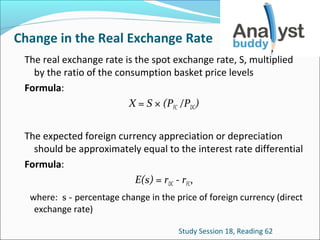
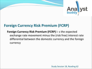
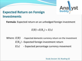
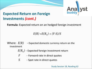
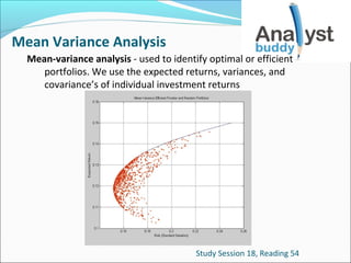
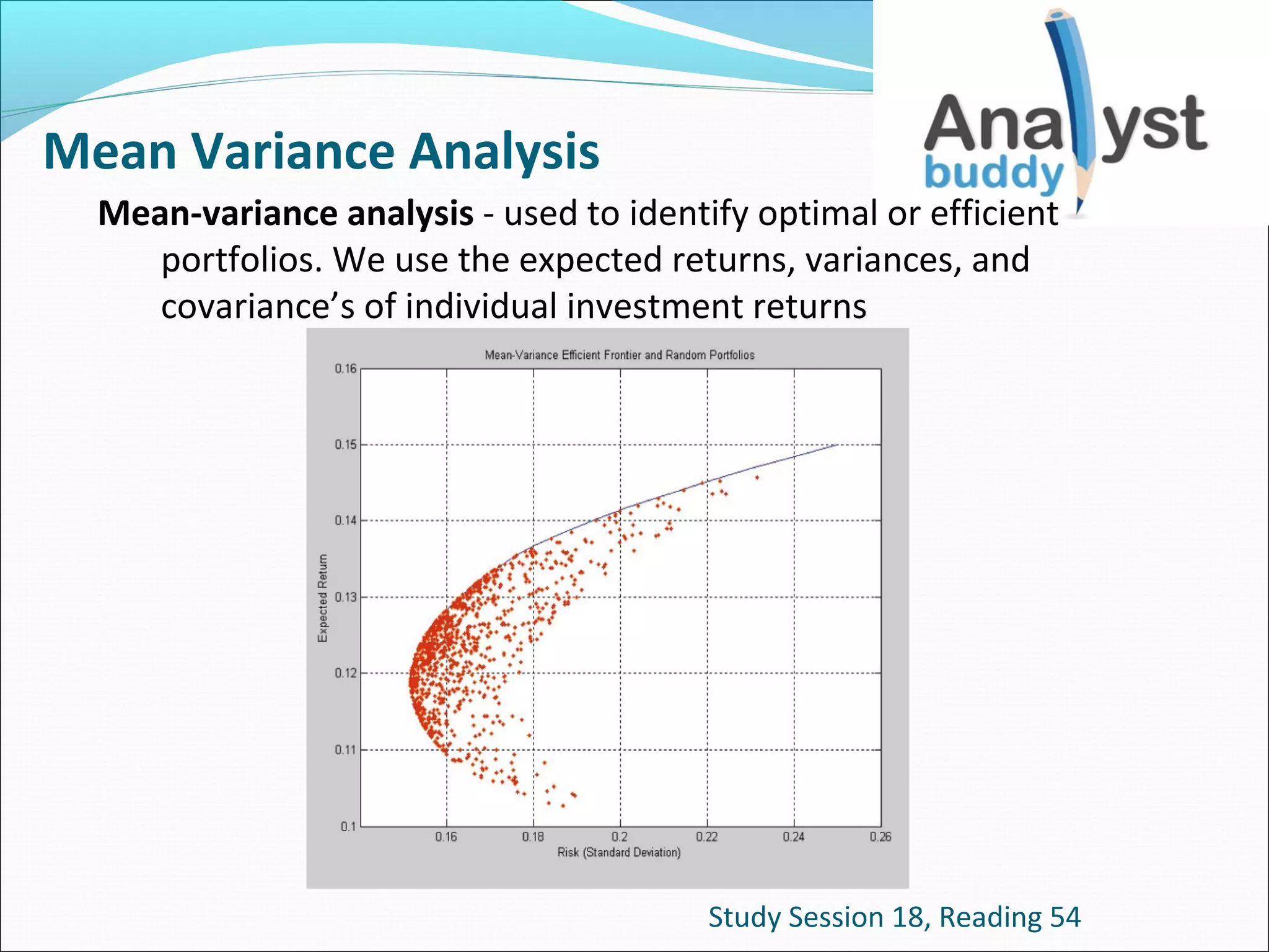
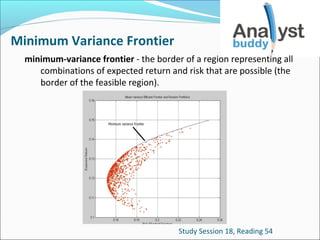
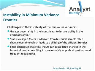
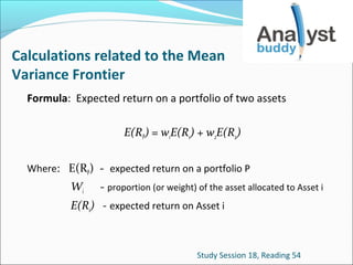
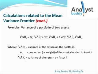
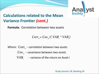
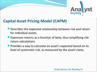
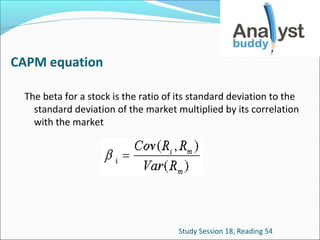
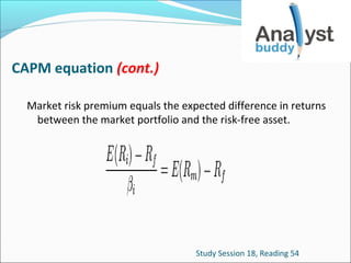
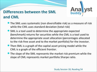
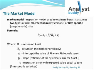
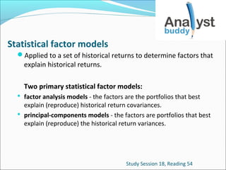
Mean-variance analysis is used to identify optimal portfolios based on expected returns, variances, and covariances of asset returns. The minimum-variance frontier shows the efficient combinations of expected return and risk. The efficient frontier begins with the global minimum-variance portfolio and provides the maximum expected return for a given level of variance. The capital market line describes combinations of the risk-free asset and market portfolio. The capital asset pricing model expresses expected returns as a linear function of systematic risk measured by beta.

1. Mean Variance Analysis
Mean-variance analysis - used to identify optimal or efficient
portfolios. We use the expected returns, variances, and
covariance’s of individual investment returns
Study Session 18, Reading 54

2. Assumptions underlying
Mean Variance Analysis
1. All investors are risk averse (ie they prefer less risk to more
2.
3.
4.
5.
for the same level of expected return)
Expected returns for all assets are known
The variance and covariance of all asset returns are known
Investors only need to know the expected returns, variances,
and covariance’s of returns to determine optimal portfolios.
They can ignore skewness, kurtosis, and other attributes of a
distribution.
There are no transaction costs or taxes
Study Session 18, Reading 54

3. Minimum Variance Frontier
minimum-variance frontier - the border of a region representing all
combinations of expected return and risk that are possible (the
border of the feasible region).
Study Session 18, Reading 54

4. Minimum Variance Frontier(cont.)
minimum-variance portfolio - one that has the smallest variance
among all portfolios with identical expected return
Steps in getting minimum-variance frontier :
1. Estimation step
2. Optimization step
Formula:
1. The portfolio weights sum to 100%:
Study Session 18, Reading 54

5. The Efficient Frontier
efficient frontier - the portion of the minimum-variance frontier
beginning with the global minimum-variance portfolio and
continuing above it
 Provides the maximum expected return for a given level of
variance
 Represents all combinations of mean return and variance or
standard deviation of return
 Investor’s portfolio selection task is greatly simplified
Study Session 18, Reading 54

6. The Efficient Frontier(cont.)
Qualities of an efficient portfolios:
Minimum risk of all portfolios with the same expected return.
Maximum expected return for all portfolios with the same
risk.
Study Session 18, Reading 54

7. Instability in Minimum Variance
Frontier
Challenges in the instability of the minimum variance :
Greater uncertainty in the inputs leads to less reliability in the
efficient frontier
Statistical input forecasts derived from historical sample often
change over time which leads to a shifting of the efficient frontier
Small changes in statistical inputs can cause large changes in the
historical frontier resulting in unreasonably large short positions and
frequent rebalancing
Study Session 18, Reading 54

8. Calculations related to the Mean
Variance Frontier
Formula: Expected return on a portfolio of two assets
E(RP) = w1E(R1) + w2E(R2)
Where: E(RP) - expected return on a portfolio P
Wi
- proportion (or weight) of the asset allocated to Asset i
E(Ri) - expected return on Asset i
Study Session 18, Reading 54

9. Calculations related to the Mean
Variance Frontier (cont.)
Formula: Variance of a portfolio of two assets
VARp2 = w12 VAR12 + w22 VAR22 + 2w1w2 VAR1 VAR2
Where: VARp - variance of the return on the portfolio
wi
- proportion (or weight) of the asset allocated to Asset i
VARi - variance of the return on Asset i
Study Session 18, Reading 54

10. Calculations related to the Mean
Variance Frontier (cont.)
Formula: Correlation between two assets
Corr1,2 = Cov1,2 /( VAR1 * VAR2)
Where: Corr1,2 - correlation between two assets
Cov1,2 - covariance between two assets
VARi
- variance of the return on Asset i
Study Session 18, Reading 54

11. Effect of Correlation on Portfolio
Diversification
Diversification - to the strategy of reducing risk by combining
many different types of assets
When the correlation between the returns on two assets is
less than +1, the potential exists for diversification benefits.
As the correlation between two assets decreases, the benefits
of diversification
When two assets have a correlation of -1, a portfolio of the
two assets exists that eliminates risk (is risk free).
If the correlation between two assets declines, the efficient
frontier improves.
Study Session 18, Reading 54

12. Effect of Number of Assets on
Portfolio Diversification
Diversification benefits increase as the number of assets
increases.
Portfolio risk will fall at a decreasing rate, as the number of
assets included in the portfolio rises.
The standard deviation of a large, well-diversified portfolio
will get closer and closer to the broad market standard
deviation as the number of assets in the portfolio increases.
Study Session 18, Reading 54

13. Equally Weighted Portfolio Risk
Formula: Variance of an equally-weighted portfolio
VARp2 = (1/n)* VARi2 + {(n-1)/n}* COV
Where : VARp - variance of the return on the portfolio
n - number of assets in the portfolio
COV - average covariance of all pairings of assets in a portfolio
Portfolio variance is affected by the number of assets in a
portfolio and the correlation between the assets
Study Session 18, Reading 54

14. Capital Allocation Line (CAL)
capital allocation line (CAL) - describes the combinations of expected
return and standard deviation of returns available to an investor
from combining the optimal portfolio of risky assets with the riskfree asset
Study Session 18, Reading 54

15. Capital Allocation Line Equation
Formula:
E(Rc) = Rf + (E(RT) – Rf)* STDEVc
STDEVT
Where: E(Rc) - expected return on an investment combination
Rf
- risk free rate of return
E(RT) - expected return on the optimal risky portfolio
STDEVc - standard deviation of the combination portfolio
STDEVT - standard deviation of the optimal risky portfolio
Study Session 18, Reading 54

16. Capital Market Line
Capital Market Line (CML) - capital allocation line in a world in which
all investors agree on the expected returns, standard deviations,
and correlations of all portfolio risk will fall at a decreasing rate, as
the number of assets included in the portfolio rises.
Formula:
E(Rc) = Rf + (E(RM) – Rf)* STDEVc
STDEVM
Where: E(Rc) - expected return on an investment combination
Rf
E(RM)
- risk free rate of return
- expected return on the market portfolio
STDEVc - standard deviation of the combination portfolio
STDEVM - standard deviation of the market portfolio
Study Session 18, Reading 54

17. Capital Asset Pricing Model (CAPM)
Describes the expected relationship between risk and return
for individual assets.
Expresses returns as a function of beta, thus simplifying risk
return calculations
Provides a way to calculate an asset’s expected based on its
level of systematic risk, as measured by the asset’s beta.
Study Session 18, Reading 54

18. Security Market Line (SML)
Security Market Line (SML) - graph of the CAPM representing the
cross-sectional relationship between the expected return for
individual assets and portfolios and their systematic risk. The
intercept equals the risk free rate and the slope equals the market
risk premium.
Study Session 18, Reading 54

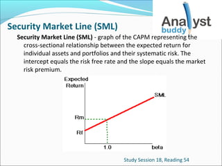
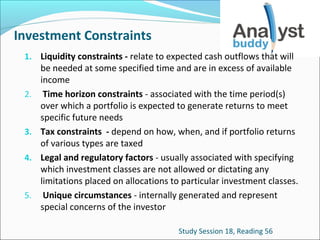
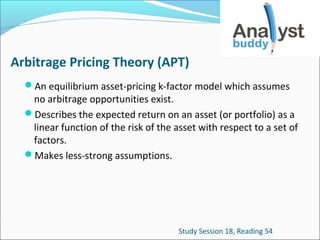
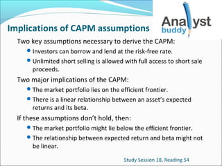
19. Security Market Line (SML) (cont.)
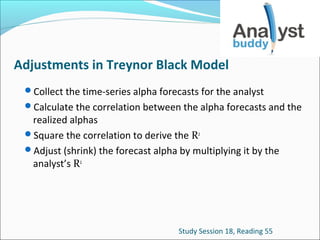
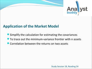
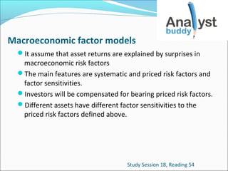
Security Market Line (SML) Equation:
E(Ri) = RF + βi[E(RM – RF)]
Where: E(Ri) - expected return on the asset
RF
- risk free rate of return
βi
- beta of the asset
E(RM – RF)]- expected risk premium
Study Session 18, Reading 54

20. CAPM equation
The beta for a stock is the ratio of its standard deviation to the
standard deviation of the market multiplied by its correlation
with the market
Study Session 18, Reading 54

21. CAPM equation (cont.)
Market risk premium equals the expected difference in returns
between the market portfolio and the risk-free asset.
Study Session 18, Reading 54

22. Differences between the SML
and CML
The SML uses systematic (non diversifiable risk) as a measure of risk
while the CML uses standard deviation (total risk)
SML is a tool used to determine the appropriate expected
(benchmark) returns for securities while the CML is a tool used to
determine the appropriate asset allocation (percentages allocated
to the risk-free asset and to the market portfolio) for the investor.
Then SML is a graph of the capital asset pricing model while the
CML is a graph of the efficient frontier.
The slope of the SML represents the market risk premium while the
slope of CML represents market portfolio Sharpe ratio.
Study Session 18, Reading 54

23. The Market Model
market model - regression model used to estimate betas. It assumes
two types of risk: macroeconomic (systematic) or firm specific
(unsystematic) risks
Formula:
Ri = αi + βi*RM + εi
Where: Ri - return on Asset i
RM - return on the market Portfolio M
αi - intercept (the value of Ri when RM equals zero)
βi - slope (estimate of the systematic risk for Asset i)
εi - regression error with expected value equal to zero
(firm-specific surprises)
Study Session 18, Reading 54

24. Underlying Assumptions of the
Market Model
The expected value of the error term is zero.
The errors are uncorrelated with the market return.
The firm-specific surprises are uncorrelated across assets.
Study Session 18, Reading 54

25. Market Model Predictions
The expected return on Asset i depends only on the expected
return on the market portfolio, E(RM), the sensitivity of the
returns on Asset i to movements in the market, βi, and the
average return to Asset i when the market return is zero, αi.
The variance of the returns on Asset i consists of two
components: a systematic component related to the asset’s
beta, βi σM , and an unsystematic component related to firmspecific events.
The covariance between any two stocks is calculated as the
product of their betas and the variance of the market
portfolio.
Study Session 18, Reading 54

26. Application of the Market Model
Simplify the calculation for estimating the covariances
To trace out the minimum-variance frontier with n assets
Correlation between the returns on two assets
Study Session 18, Reading 54

27. Calculation of Adjusted
and Historical Beta
Historical beta is calculated by the use of the historical
regression estimate derived from the market model.
Often some adjustments are made to the historical beta to
improve its ability to forecast the future beta.
Adjusted beta is a historical beta adjusted to reflect the
tendency of beta to mean revert (towards one).
An adjusted beta tends to predict future beta better than
historical beta does.
Study Session 18, Reading 54

28. Multifactor Models
Describe the return of an asset in terms of the risk of the
asset with respect to a set of factors.
Include systematic factors, which explain the average returns
of a large number of risky assets.
Categories:
 macroeconomic factor models
 fundamental factor models
 statistical factor models
Study Session 18, Reading 54

29. Macroeconomic factor models
It assume that asset returns are explained by surprises in
macroeconomic risk factors
The main features are systematic and priced risk factors and
factor sensitivities.
Investors will be compensated for bearing priced risk factors.
Different assets have different factor sensitivities to the
priced risk factors defined above.
Study Session 18, Reading 54

30. Macroeconomic factor models
(cont.)
Formula: Return for stocks using macroeconomic model
Formula: Return on portfolio using two-factor macroeconomic
factor mode
Study Session 18, Reading 54

31. Fundamental factor models
It assume that asset returns are explained by multiple firm
specific factors.
Sensitivities are not regression slopes. Instead, the
sensitivities are standardized attributes
The fundamental factors are rates of return associated with
each factor
Study Session 18, Reading 54

32. Statistical factor models
Applied to a set of historical returns to determine factors that
explain historical returns.
Two primary statistical factor models:
 factor analysis models - the factors are the portfolios that best
explain (reproduce) historical return covariances.
 principal-components models - the factors are portfolios that best
explain (reproduce) the historical return variances.
Study Session 18, Reading 54

33. Arbitrage Pricing Theory (APT)
An equilibrium asset-pricing k-factor model which assumes
no arbitrage opportunities exist.
Describes the expected return on an asset (or portfolio) as a
linear function of the risk of the asset with respect to a set of
factors.
Makes less-strong assumptions.
Study Session 18, Reading 54

34. Assumptions of APT
Returns are derived from a multifactor model.
Unsystematic risk can be completely diversified away.
No arbitrage opportunities exist
arbitrage opportunity - an investment opportunity that bears
no risk, no cost, and yet provides a profit
Study Session 18, Reading 54

35. APT Equation
Study Session 18, Reading 54

36. Differences between APT and
Multifactor Models
Arbitrage Pricing Theory (APT) models look similar to
multifactor models
While APT models are equilibrium models, multifactor
models are statistical regressions
APT models explain the results over a single time period as
functions of different factors, while multifactor models are
based on data from multiple time periods
Study Session 18, Reading 54

37. Active Risk and Return,
Information Ration
Active return - return in excess of the return of the benchmark
Formula:
Active Return = RP – RB
Active risk - the standard deviation of active returns.
Components:
 Active factor risk
 Active specific risk
Information ratio standardizes the return achieved by a
portfolio manager by dividing the return with the standard
deviation of the return.
Study Session 18, Reading 54

38. Factor and Tracking Portfolios
pure factor portfolio (or simply a factor portfolio) - a portfolio
that has been constructed to have a sensitivity equal to 1.0 to
only one risk factor, and sensitivities of zero to the remaining
factors.
tracking portfolios - have a deliberately designed set of factor
exposures. That is, a tracking portfolio is deliberately
constructed to have the same set of factor exposures to
match (“track”) a predetermined benchmark.
Study Session 18, Reading 54

39. Implications of CAPM assumptions
Two key assumptions necessary to derive the CAPM:
 Investors can borrow and lend at the risk-free rate.
 Unlimited short selling is allowed with full access to short sale
proceeds.
Two major implications of the CAPM:
 The market portfolio lies on the efficient frontier.
 There is a linear relationship between an asset’s expected
returns and its beta.
If these assumptions don’t hold, then:
 The market portfolio might lie below the efficient frontier.
 The relationship between expected return and beta might not
be linear.
Study Session 18, Reading 54

40. Impediments to Market Integration
Psychological barriers
Legal restrictions
Transaction costs
Discriminatory taxation
Political risks
Foreign currency risk
Study Session 18, Reading 54

41. Factors favouring Market
Integration
There are many private and institutional investors who are
internationally active.
Many major corporations have multinational operations.
Corporations and governments borrow and lend on an
international scale.
Study Session 18, Reading 62

42. Extended CAPM
extended CAPM - domestic CAPM extended to the international
environment is called the
The risk-free rate (Rf) is the investor’s domestic risk-free rate,
and the market portfolio is the market capitalizationweighted portfolio of all risky assets in the world
Assumptions needed to extend CAPM
Investors throughout the world have identical consumption
baskets.
 Purchasing power parity holds exactly at any point in time.
Study Session 18, Reading 62

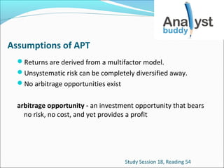
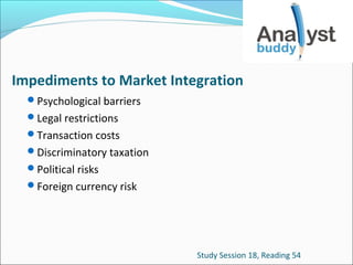
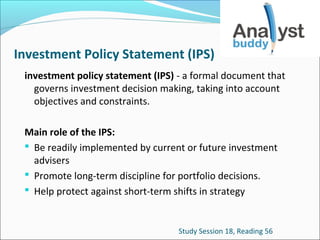
43. ICAPM Equation
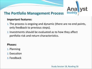
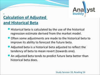
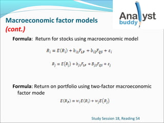
E(r)= Rf +(βg×MrPg )+(g1×FcrP1)+(g2×FcrP2 )+...........+(gk ×FcrPk )
Where: E(r) - asset’s expected return
Rrf - domestic currency risk-free rate
βg - sensitivity of the asset’s domestic currency returns to
changes in the global market portfolio
MrPg - world market risk premium [E(rm ) - r ]
E(r m) - expected return on world market portfolio
g1 to gk - sensitivities of asset’s domestic currency returns to
changes in the values of currencies 1 through k
FcrP1 to FcrPk - foreign currency risk premiums on
currencies 1 through k
Study Session 18, Reading 62

44. Change in the Real Exchange Rate
The real exchange rate is the spot exchange rate, S, multiplied
by the ratio of the consumption basket price levels
Formula:
X = S × (PFC /PDC)
The expected foreign currency appreciation or depreciation
should be approximately equal to the interest rate differential
Formula:
E(s) = rDC - rFC,
where: s - percentage change in the price of foreign currency (direct
exchange rate)
Study Session 18, Reading 62

45. Foreign Currency Risk Premium (FCRP)
Foreign Currency Risk Premium (FCRP) i- s the expected
exchange rate movement minus the (risk free) interest rate
differential between the domestic currency and the foreign
currency
Study Session 18, Reading 62

46. Expected Return on Foreign
Investments
Formula: Expected return on an unhedged foreign investment
E(R) =E(RFC) + E(s)
Where: E(R) - Expected domestic currency return on the investment
E(RFC) - Expected foreign investment return
E(s)
- Expected percentage currency movement
Study Session 18, Reading 62

47. Expected Return on Foreign
Investments (cont.)
Formula: Expected return on an hedged foreign investment
E(R) =E(RFC) + (F-S)/S
Where: E(R)
investment
- Expected domestic currency return on the
E(RFC) - Expected foreign investment return
F
S
- Forward rate in direct quotes
- Spot rate in direct quotes
Study Session 18, Reading 62

48. Currency Exposure
local currency exposure – the sensitivity of the returns in the
stock denominated in the local currency to changes in the
value of the local currency
domestic currency exposure - because the exposure of a
currency to itself is 1, domestic currency exposure is equal to
local currency exposure plus 1.
Study Session 18, Reading 62

49. Exchange Rate Exposure
exchange rate exposure – the way the value of an individual
company changes in response to a change in the real value of
the local currency
We can estimate the currency exposure of a particular firm
by regressing the firm’s stock return on local currency
changes.
Study Session 18, Reading 62

50. Economic activity and exchange rate
movements
Two theories to explain the relationship between economic
activity and exchange rate:
1. traditional model - predicts that depreciation in the value of
the domestic currency will cause an increase in the
competitiveness of the domestic industry and, thus, an
increase in the stock value of domestic firms
2. money demand model - an increase in real economic activity
leads to an increase in the demand for the domestic currency
Study Session 18, Reading 62

51. Active portfolio management
active portfolio management - refers to decisions of the
portfolio manager to actively manage and monitor the broad
asset allocation and security selection of the portfolio.
Equilibrium is the desirable end result of active portfolio
management.
Study Session 18, Reading 55

52. Justification of active portfolio
management
Develop capital market forecasts for major asset classes
Allocate funds across the major risky asset classes to form the
optimal risky portfolio that maximizes the reward-to-risk
ratio.
Allocate funds between the risk-free asset and the optimal
risky portfolio in order to satisfy the investor’s risk aversion.
Rebalance the portfolio as capital market forecasts and
investor’s risk aversion changes (also known as market timing)
Study Session 18, Reading 55

53. Treynor Black Model
Treynor-Black model - a portfolio optimization framework that
combines market inefficiency and modern portfolio theory.
The model is based on the premise that markets are nearly
efficient.
Objective: To create an optimal risky portfolio that is allocated
to both a passively managed (indexed) portfolio and to an
actively managed portfolio
Formula:
Study Session 18, Reading 55

54. Adjustments in Treynor Black Model
Collect the time-series alpha forecasts for the analyst
Calculate the correlation between the alpha forecasts and the
realized alphas
Square the correlation to derive the R2
Adjust (shrink) the forecast alpha by multiplying it by the
analyst’s R2
Study Session 18, Reading 55

55. The Portfolio Management Process
Important features:
1. The process is ongoing and dynamic (there are no end points,
only feedback to previous steps).
2. Investments should be evaluated as to how they affect
portfolio risk and return characteristics.
Phases:
1. Planning
2. Execution
3. Feedback
Study Session 18, Reading 56

56. Investment Constraints
1. Liquidity constraints - relate to expected cash outflows that will
2.
3.
4.
5.
be needed at some specified time and are in excess of available
income
Time horizon constraints - associated with the time period(s)
over which a portfolio is expected to generate returns to meet
specific future needs
Tax constraints - depend on how, when, and if portfolio returns
of various types are taxed
Legal and regulatory factors - usually associated with specifying
which investment classes are not allowed or dictating any
limitations placed on allocations to particular investment classes.
Unique circumstances - internally generated and represent
special concerns of the investor
Study Session 18, Reading 56

57. Investment Policy Statement (IPS)
investment policy statement (IPS) - a formal document that
governs investment decision making, taking into account
objectives and constraints.
Main role of the IPS:
 Be readily implemented by current or future investment
advisers
 Promote long-term discipline for portfolio decisions.
 Help protect against short-term shifts in strategy
Study Session 18, Reading 56

58. Elements of the IPS
A client description
Identification of duties and responsibilities of parties
involved.
The formal statement of objectives and constraints.
A calendar schedule for both portfolio performance and IPS
review.
Asset allocation ranges and statements regarding flexibility
and rigidity when formulating or modifying the strategic asset
allocation.
Guidelines for portfolio adjustments and rebalancing.
Study Session 18, Reading 56

59. Strategic Asset Allocation
Strategic asset allocation is the final step in the planning stage.
Common Approaches to Strategic Asset Allocation
1. Passive investment strategies – represent strategies that are
not responsive to changes in expectations
2. Active investment strategies - attempt to capitalize on
differences between a portfolio manager’s beliefs concerning
security valuations and those in the marketplace.
3. Semi-active, risk-controlled active, or enhanced index
strategies - hybrids of passive and active strategies
Study Session 18, Reading 56

60. Factors affecting Strategic Asset
Allocation
1. Risk-return
2. Capital market expectations
3. The length of the time horizon
Affect of Time Horizon:
The longer the investment time horizon, the more risk an
investor can take on
Study Session 18, Reading 56