CAPM & Efficient Market Hypothesis presentation

1. @ Ravindra Nath Shukla
Capital Assets Pricing Model
and
Efficient Market Hypothesis

2. LEARNING OBJECTIVES
 Discuss the concepts of portfolio risk and return
 Determine the relationship between risk and return of
portfolios
 Highlight the difference between systematic and
unsystematic risks
 Examine the logic of portfolio theory
 Show the use of capital asset pricing model (CAPM) in the
valuation of securities
 Explain the features and modus operandi of the arbitrage
pricing theory (APT)
2

3. INTRODUCTION
 A portfolio is a bundle or a combination of individual assets or securities.
 Portfolio theory provides a normative approach to investors to make
decisions to invest their wealth in assets or securities under risk
 Extend the portfolio theory to derive a framework for valuing risky assets.
This framework is referred to as the capital asset pricing model (CAPM).
An alternative model for the valuation of risky assets is the arbitrage
pricing theory (APT).
 The return of a portfolio is equal to the weighted average of the returns
of individual assets (or securities)
3

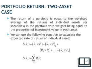
4. PORTFOLIO RETURN: TWO-ASSET
CASE
 The return of a portfolio is equal to the weighted
average of the returns of individual assets (or
securities) in the portfolio with weights being equal to
the proportion of investment value in each asset.
 We can use the following equation to calculate the
expected rate of return of individual asset:
4

5. Expected Rate of Return:
Example
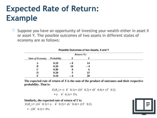
 Suppose you have an opportunity of investing your wealth either in asset X
or asset Y. The possible outcomes of two assets in different states of
economy are as follows:
Possible Outcomes of two Assets, X and Y
Return (%)
State of Economy Probability X Y
A 0.10 – 8 14
B 0.20 10 – 4
C 0.40 8 6
D 0.20 5 15
E 0.10 – 4 20
The expected rate of return of X is the sum of the product of outcomes and their respective
probability. That is:
( ) ( 8 0.1) (10 0.2) (8 0.4) (5 0.2)
( 4 0.1) 5%
x
E R = - ´ + ´ + ´ + ´
+ - ´ =
Similarly, the expected rate of return of Y is:
( ) (14 0.1) ( 4 0.2) (6 0.4) (15 0.2)
(20 0.1) 8%
y
E R = ´ + - ´ + ´ + ´
+ ´ =
5

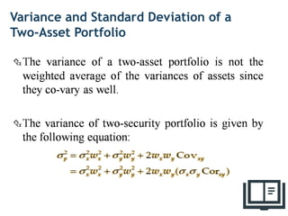
6. PORTFOLIO RISK: TWO-ASSET CASE
 Risk of individual assets is measured by their variance
or standard deviation.
 We can use variance or standard deviation to measure
the risk of the portfolio of assets as well.
 The risk of portfolio would be less than the risk of
individual securities, and that the risk of a security
should be judged by its contribution to the portfolio
risk.
6

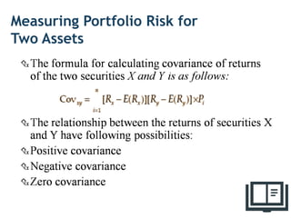
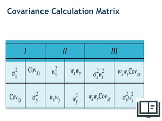
7. Measuring Portfolio Risk for
Two Assets
 The portfolio variance or standard deviation depends
on the co-movement of returns on two assets.
 Covariance of returns on two assets measures their co-
movement.
 Three steps are involved in the calculation of
covariance between two assets:
7

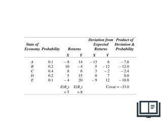
8. Deviation from Product of
State of Expected Deviation &
Economy Probability Returns Returns Probability
X Y X Y
A 0.1 – 8 14 – 13 6 – 7.8
B 0.2 10 – 4 5 – 12 – 12.0
C 0.4 8 6 3 – 2 – 2.4
D 0.2 5 15 0 7 0.0
E 0.1 – 4 20 – 9 12 – 10.8
E(RX
) E(RY
) Covar = –33.0
= 5 = 8
8

9. Example
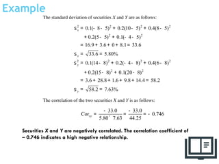
The standard deviation of securities X and Y are as follows:
2 2 2 2
2 2
2 2 2 2
2 2
0.1( 8 5) 0.2(10 5) 0.4(8 5)
0.2(5 5) 0.1( 4 5)
16.9 3.6 0 8.1 33.6
33.6 5.80%
0.1(14 8) 0.2( 4 8) 0.4(6 8)
0.2(15 8) 0.1(20 8)
3.6 28.8 1.6 9.8 14.4 58.2
58.2 7.63%
x
x
y
y
s = - - + - + -
+ - + - -
= + + + =
s = =
s = - + - - + -
+ - + -
= + + + + =
s = =
The correlation of the two securities X and Y is as follows:
33.0 33.0
Cor 0.746
5.80 7.63 44.25
xy
- -
= = = -
´
9
Securities X and Y are negatively correlated. The correlation coefficient of
– 0.746 indicates a high negative relationship.

10. Measuring Portfolio Risk for
Two Assets
10

11. Correlation
11

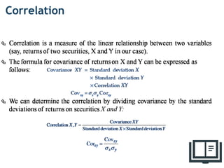
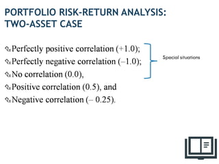
12. Correlation
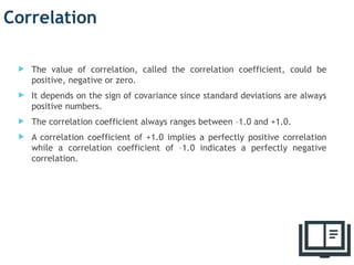
 The value of correlation, called the correlation coefficient, could be
positive, negative or zero.
 It depends on the sign of covariance since standard deviations are always
positive numbers.
 The correlation coefficient always ranges between –1.0 and +1.0.
 A correlation coefficient of +1.0 implies a perfectly positive correlation
while a correlation coefficient of –1.0 indicates a perfectly negative
correlation.
12

13. Variance and Standard Deviation of a
Two-Asset Portfolio
13

14. Covariance Calculation Matrix
14

15. Minimum Variance Portfolio
15

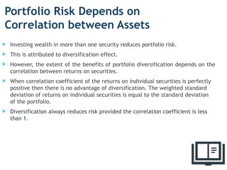
16. Portfolio Risk Depends on
Correlation between Assets
 Investing wealth in more than one security reduces portfolio risk.
 This is attributed to diversification effect.
 However, the extent of the benefits of portfolio diversification depends on the
correlation between returns on securities.
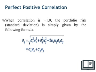
 When correlation coefficient of the returns on individual securities is perfectly
positive then there is no advantage of diversification. The weighted standard
deviation of returns on individual securities is equal to the standard deviation
of the portfolio.
 Diversification always reduces risk provided the correlation coefficient is less
than 1.
16

17. PORTFOLIO RISK-RETURN ANALYSIS:
TWO-ASSET CASE
17

18. Perfect Positive Correlation
18

19. 19
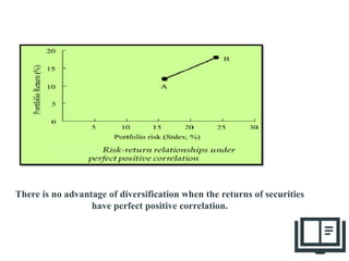
There is no advantage of diversification when the returns of securities
have perfect positive correlation.

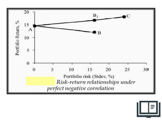
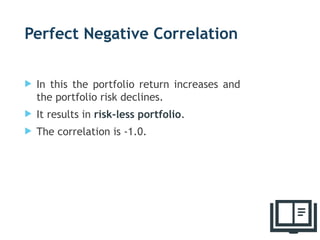
20. Perfect Negative Correlation
 In this the portfolio return increases and
the portfolio risk declines.
 It results in risk-less portfolio.
 The correlation is -1.0.
20

21. 21

22. Zero-variance portfolio
22

23. Zero Correlation
23

24. 24

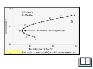
25. Positive Correlation
 In reality, returns of most assets have
positive but less than 1.0 correlation.
25

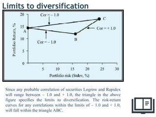
26. Limits to diversification
26
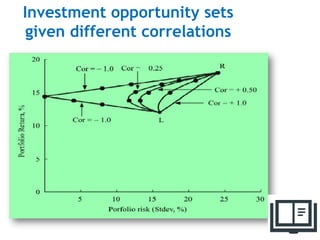
Since any probable correlation of securities Logrow and Rapidex
will range between – 1.0 and + 1.0, the triangle in the above
figure specifies the limits to diversification. The risk-return
curves for any correlations within the limits of – 1.0 and + 1.0,
will fall within the triangle ABC.

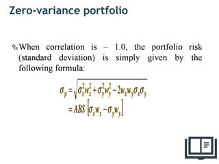
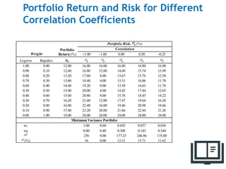
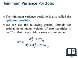
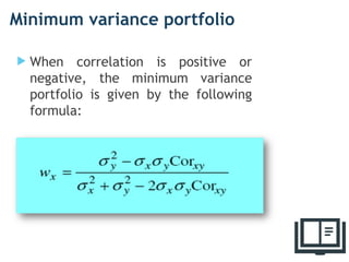
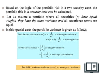
27. Minimum variance portfolio
 When correlation is positive or
negative, the minimum variance
portfolio is given by the following
formula:
27

28. EFFICIENT PORTFOLIO AND
MEAN-VARIANCE CRITERION
28

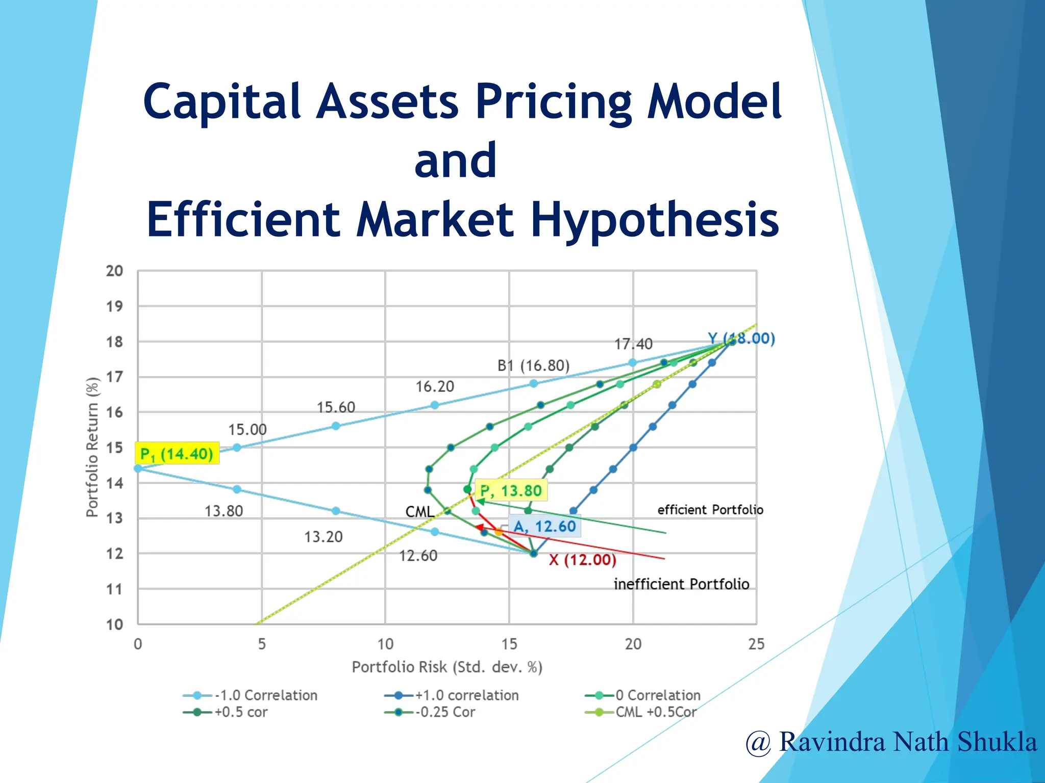
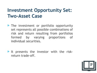
29. Investment Opportunity Set:
Two-Asset Case
 The investment or portfolio opportunity
set represents all possible combinations of
risk and return resulting from portfolios
formed by varying proportions of
individual securities.
 It presents the investor with the risk-
return trade-off.
29

30. Portfolio Return and Risk for Different
Correlation Coefficients
Portfolio Risk, p (%)
Correlation
Weight
Portfolio
Return (%) +1.00 -1.00 0.00 0.50 -0.25
Logrow Rapidex Rp p p p p p
1.00 0.00 12.00 16.00 16.00 16.00 16.00 16.00
0.90 0.10 12.60 16.80 12.00 14.60 15.74 13.99
0.80 0.20 13.20 17.60 8.00 13.67 15.76 12.50
0.70 0.30 13.80 18.40 4.00 13.31 16.06 11.70
0.60 0.40 14.40 19.20 0.00 13.58 16.63 11.76
0.50 0.50 15.00 20.00 4.00 14.42 17.44 12.65
0.40 0.60 15.60 20.80 8.00 15.76 18.45 14.22
0.30 0.70 16.20 21.60 12.00 17.47 19.64 16.28
0.20 0.80 16.80 22.40 16.00 19.46 20.98 18.66
0.10 0.90 17.40 23.20 20.00 21.66 22.44 21.26
0.00 1.00 18.00 24.00 24.00 24.00 24.00 24.00
Minimum Variance Portfolio
wL 1.00 0.60 0.692 0.857 0.656
wR 0.00 0.40 0.308 0.143 0.344
2
256 0.00 177.23 246.86 135.00
 (%) 16 0.00 13.31 15.71 11.62
30

31. Investment opportunity sets
given different correlations
31

32. Mean-variance Criterion
 Inefficient portfolios- have lower return and
higher risk
32

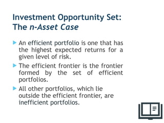
33. Investment Opportunity Set:
The n-Asset Case
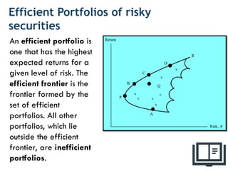
 An efficient portfolio is one that has
the highest expected returns for a
given level of risk.
 The efficient frontier is the frontier
formed by the set of efficient
portfolios.
 All other portfolios, which lie
outside the efficient frontier, are
inefficient portfolios.
33

34. Efficient Portfolios of risky
securities
34
An efficient portfolio is
one that has the highest
expected returns for a
given level of risk. The
efficient frontier is the
frontier formed by the
set of efficient
portfolios. All other
portfolios, which lie
outside the efficient
frontier, are inefficient
portfolios.

35. PORTFOLIO RISK: THE n-
ASSET CASE
 The calculation of risk becomes quite involved when a
large number of assets or securities are combined to
form a portfolio.
35

36. N-Asset Portfolio Risk Matrix
36

37. 37

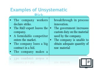
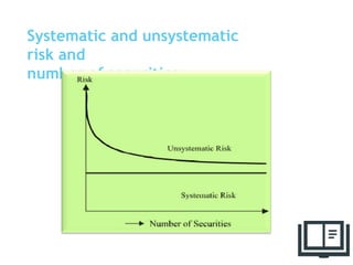
38. RISK DIVERSIFICATION:
SYSTEMATIC AND UNSYSTEMATIC
RISK
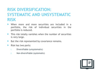
 When more and more securities are included in a
portfolio, the risk of individual securities in the
portfolio is reduced.
 This risk totally vanishes when the number of securities
is very large.
 But the risk represented by covariance remains.
 Risk has two parts:
1. Diversifiable (unsystematic)
2. Non-diversifiable (systematic)
38

39. Systematic Risk
 Systematic risk arises on account of the economy-wide uncertainties and
the tendency of individual securities to move together with changes in
the market.
 This part of risk cannot be reduced through diversification.
 It is also known as market risk.
 Investors are exposed to market risk even when they hold well-diversified
portfolios of securities.
39

40. Examples of Systematic Risk
40

41. Unsystematic Risk
 Unsystematic risk arises from the unique uncertainties of individual
securities.
 It is also called unique risk.
 These uncertainties are diversifiable if a large numbers of securities are
combined to form well-diversified portfolios.
 Uncertainties of individual securities in a portfolio cancel out each other.
 Unsystematic risk can be totally reduced through diversification.
41

42. Examples of Unsystematic
Risk
42

43. Total Risk
43

44. Systematic and unsystematic
risk and
number of securities
44

45. COMBINING A RISK-FREE ASSET
AND
A RISKY ASSET
45

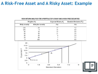
46. A Risk-Free Asset and A Risky Asset: Example
RISK-RETURN ANALYSIS FOR A PORTFOLIO OF A RISKY AND A RISK-FREE SECURITIES
Weights (%) Expected Return, Rp
Standard Deviation (p)
Risky security Risk-free security (%) (%)
120 – 20 17 7.2
100 0 15 6.0
80 20 13 4.8
60 40 11 3.6
40 60 9 2.4
20 80 7 1.2
0 100 5 0.0
0
2.5
5
7.5
10
12.5
15
17.5
20
0 1.8 3.6 5.4 7.2 9
Standard Deviation
E
x
p
e
c
te
d
R
e
tu
r
n
A
B
C
D
Rf, risk-free rate

47. Borrowing and Lending
47
Risk-return relationship for portfolio of risky and risk-free securities

48. MULTIPLE RISKY ASSETS AND
A RISK-FREE ASSET
 In a market situation, a large number of investors
holding portfolios consisting of a risk-free security and
multiple risky securities participate.
48

49. 49
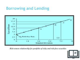
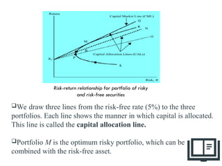
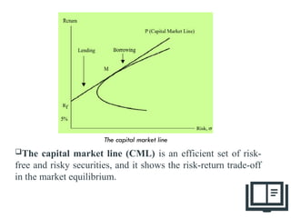
We draw three lines from the risk-free rate (5%) to the three
portfolios. Each line shows the manner in which capital is allocated.
This line is called the capital allocation line.
Portfolio M is the optimum risky portfolio, which can be
combined with the risk-free asset.
Risk-return relationship for portfolio of risky
and risk-free securities

50. 50
The capital market line (CML) is an efficient set of risk-
free and risky securities, and it shows the risk-return trade-off
in the market equilibrium.
The capital market line

51. Separation Theory
 According to the separation theory, the choice of
portfolio involves two separate steps.
 The first step involves the determination of the
optimum risky portfolio.
 The second step concerns with the investor’s decision to
form portfolio of the risk-free asset and the optimum
risky portfolio depending on her risk preferences.
51

52. Slope of CML
52

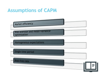
53. CAPITAL ASSET PRICING
MODEL (CAPM)
 The capital asset pricing model (CAPM) is a model that
provides a framework to determine the required rate of
return on an asset and indicates the relationship between
return and risk of the asset.
 The required rate of return specified by CAPM helps in
valuing an asset.
 One can also compare the expected (estimated) rate of
return on an asset with its required rate of return and
determine whether the asset is fairly valued.
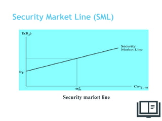
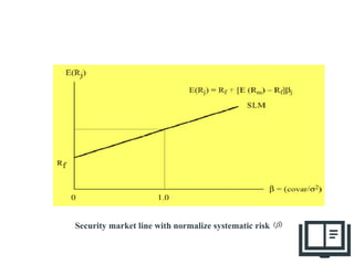
 Under CAPM, the security market line (SML) exemplifies
the relationship between an asset’s risk and its required
rate of return.
53

54. Assumptions of CAPM
54

55. Characteristics Line
55

56. Security Market Line (SML)
56
Security market line

57. 57
Security market line with normalize systematic risk

58. IMPLICATIONS AND
RELEVANCE OF CAPM
58

59. Implications
 Investors will always combine a risk-free asset with a market portfolio of
risky assets. They will invest in risky assets in proportion to their market
value.
 Investors will be compensated only for that risk which they cannot
diversify.
 Investors can expect returns from their investment according to the risk.
59

60. Limitations
 It is based on unrealistic assumptions.
 It is difficult to test the validity of CAPM.
 Betas do not remain stable over time.
60

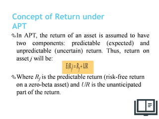
61. THE ARBITRAGE PRICING
THEORY (APT)
 The act of taking advantage of a price differential between two or more
markets is referred to as arbitrage.
 The Arbitrage Pricing Theory (APT) describes the method of bring a
mispriced asset in line with its expected price.
 An asset is considered mispriced if its current price is different from the
predicted price as per the model.
 The fundamental logic of APT is that investors always indulge in arbitrage
whenever they find differences in the returns of assets with similar risk
characteristics.
61

62. Concept of Return under
APT
62

63. Concept of Risk under APT
63

64. Steps in Calculating
Expected Return under APT
64

65. Factors
65

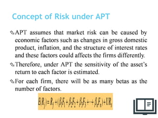
66. Risk premium
 Conceptually, it is the compensation, over and above,
the risk-free rate of return that investors require for the
risk contributed by the factor.
 One could use past data on the forecasted and actual
values to determine the premium.
66

67. Factor beta
 The beta of the factor is the sensitivity of the asset’s
return to the changes in the factor.
 One can use regression approach to calculate the factor
beta.
67