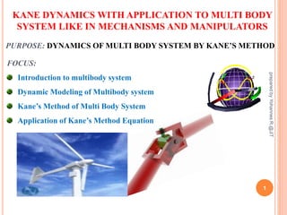
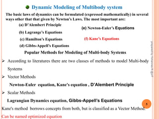
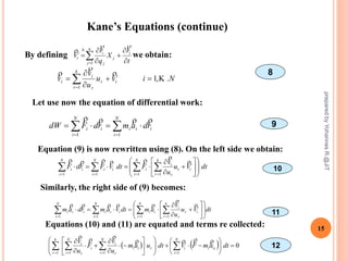
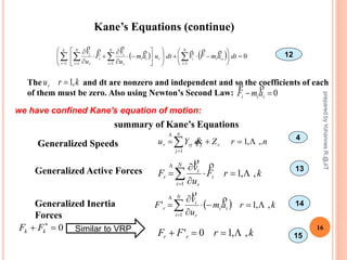
SlideShare a Scribd company logo
PURPOSE: DYNAMICS OF MULTI BODY SYSTEM BY KANE’S METHOD
FOCUS:
Introduction to multibody system
Dynamic Modeling of Multibody system
Kane’s Method of Multi Body System
Application of Kane’s Method Equation
1
KANE DYNAMICS WITH APPLICATION TO MULTI BODY
SYSTEM LIKE IN MECHANISMS AND MANIPULATORS
preparedbyYohannesR.@JiT
 In Systems where all parts are not best described in an inertial
or "world" reference frame are referred to as multi-body
systems (MBSs).
 These are common in:
Robotics
Aerospace
Aviation
Industrial Automation
2
Introduction to multibody system
preparedbyYohannesR.@JiT
 To model a given dynamic system S, one has choose variables to
describe the configuration of S, or variables that specify the
location of a reference point and orientation of a reference frame
fixed within each body of S. These variables named as
configuration variables.
 For mechanical scenario, a multibody system is a system that
consists a number of rigid bodies (referred to as links) connected in
succession by kinematic pairs (referred to as joints).
Base
Link0
Joint1
Link2
Link3Joint3
End of Arm
Link1
Joint2
3
preparedbyYohannesR.@JiT
4
 Human hands can be act as MBS in which the arrangement of bones(link) and kinematic
pair of joints provides dexterity (manipulating objects)
 Each joint represent a degree of freedom; there are 27bones, 22joints and thus 22DoF
Example of MBS
preparedbyYohannesR.@JiT
5
The basic laws of dynamics can be formulated (expressed mathematically) in several
ways other that that given by Newton’s Laws. The most important are:
(a) D’Alembert Principle
(b) Lagrange’s Equations
(c) Hamilton’s Equations (f) Kane’s Equations
(d) Gibbs-Appell’s Equations
Popular Methods for Modeling of Multi-body Systems
 According to literatures there are two classes of methods to model Multi-body
Systems
 Vector Methods
Newton-Euler equation, Kane's equation , D’Alembert Principle
 Scalar Methods
Lagrangian Dynamics equation, Gibbs-Appell’s Equations
Kane's method borrows concepts from both, but is classified as a Vector Method.
Can be named optimized equation
(e) Newton-Euler’s Equations
Dynamic Modeling of Multibody system
preparedbyYohannesR.@JiT
6
 Kane’s method (originally called Lagrange form of D'Alambert's principle)
which is a powerful tool for developing dynamical equations for MBS motion
 Applying the Newton-Euler method requires that force and moment balances
be applied for each body taking in consideration every interactive and constraint
force.
 Therefore, the method is inefficient when only a few of the system’s forces need
to be solved for.
 The major disadvantage of Lagrange’s Equations method is the need to
differentiate scalar energy functions (kinetic and potential energy).
 In Kane’s method, With the use of generalized forces the need for examining
interactive and constraint forces between bodies is eliminated
 (Huston 1990) argue that; Kane’s method provides combined means to
develop the dynamics equations for multibody systems that lends itself to
automated numerical computation.
preparedbyYohannesR.@JiT
 Essentially all methods for obtaining equations of motion are equivalent.
 However, some are more suited for multibody dynamics than others.
 For example, if a revolute joint connects two bodies, only the joint angle is
needed to describe the configuration of the second body, if the configuration
of the first is known.
 Compared to a set of variables that specifies the location and orientation of
each body relative to a common ground, a set of generalized coordinates is
reduced in number i.e., n<6v, where v is the number of bodies of S and spatial
motion is being considered.
 If M is the number of configuration constraints encapsulated by the choice of
generalized coordinates, then n = 6v-M.
 The generalized coordinates describe only the allowed configurations and thus
encapsulate certain configuration constraints.
7
preparedbyYohannesR.@JiT
 Generalized coordinates are a set of convenient coordinates, usually
independent of one another, used to describe a particular configuration of a
system
Kane's method is touted as a superior approach by it proponents
because it:
 Encapsulates holonomic (position) constraints by the use of
generalized coordinates (as in the Lagrangian method).
 Also encapsulates non- holonomic (velocity) constraints through
the use of generalized speeds. (Which requires Lagrange's Method
of Undetermined Multipliers)
 Results in a compact, first order representation of the equations of
motion. (ODE)
 Is more systematic and therefore easier to learn .
 Is becoming the industry standard where complex systems need to
be modeled.
Why Kane's Method?
8
preparedbyYohannesR.@JiT
9
Kane’s Equations
Consider an open-chain multibody system of N interconnected rigid bodies each
subject to external and constraint forces these external forces can be transformed
into an equivalent force and torque Fk and Mk passing through Gk ,which is the
mass center of the body k , (k = 1,2…N).
Similar to the external forces, the constraint forces may be written as and
Using D'Alambert's principle for the force equilibrium of body k, the following is
obtained
0  c
kkk FFF

kkk amF 

where is the inertia force of body k.
The concept of virtual work may be described as follows for a system of N
particles with N degrees of freedom
Professor Thomas R. Kane
1924 -
Stanford University
Kane’s Equations Using the Principle of Virtual Work
c
kF

c
kM

Kane’s Method of Multi Body System
preparedbyYohannesR.@JiT
10
The virtual work is then defined as:


N
i
ii rFW
1


Where is the resultant force acting on the ith particle and is the position vector of the
particle in the inertial reference frame. is the virtual displacement, which is imaginary in
the sense that it is assumed to occur without the passage of time.
iF

ir
ir
Now applying the concept of virtual work to our multibody system considering
only the work due to the forces on the system we obtain:
0)(  
k
c
kkk rFFFW 

(k = 1,2,…,N)
The constraints that are commonly encountered are known as workless constraints so…
0 k
c
k rF 

Which simplifies the virtual work equation to:
0)(  
kkki rFFW 

The positions vector may also be written as:
),( tqrr rkk


t
r
dt
dq
q
r
r kr
r
k
k








t
r
q
q
r k
r
r
k










preparedbyYohannesR.@JiT
11
Taking the partial derivative of with respect to we obtain
kr
rq
r
k
r
k
q
r
q
r








r
k
r
k
q
r
q
v








or
Since the virtual displacement is arbitrary without violating the constraints
we can write * as:
rq
0 
KK ff Kf

Kf
generalized active
generalized inertia forces
r
k
kK
q
v
Ff





r
k
kK
q
v
Ff




 
In a similar fashion it can be shown using
virtual work that the moments can be
written as
0 
KK MM
KM generalized active moments

KM generalized inertia moments
r
k
kK
q
TM






r
k
kkkK
q
IIM





 
 )(
By superposition of the force and moment
equations we arrive at Kane’s equations:
0 
kk FF
KKK MfF 

 KKK MfF
preparedbyYohannesR.@JiT
12
 tri

ir


tvi

 tPi tP i'
 ttP i '
ir


Virtual Path True Path (P)
Newtonian or
Dynamic Path
The Constraint
Space at t
mjra
N
i
i
j
i ,,10
1




   
   
   







0
0
0
21
21
21
tttt
trtr
trtr
ii
ii



1t
2t
Kane’s Equations can be also derived in terms of generalized coordinates we
can write:
Kane’s Equations Using the Generalized Coordinates system
          Niktqzjtqyitqxtqqrtqr iiinii .,1,,,,,,, 1 



 1
  Nikdzjdyidxdt
t
r
dq
q
r
tqrd iii
i
n
j
j
j
i
i .,1,
1









 
2
preparedbyYohannesR.@JiT
13
 
Ni
t
r
q
q
r
td
tqrd
rv i
n
j
j
j
ii
ii .,1
,
1












 

3
Kane and Levinson have shown that with the n generalized coordinates , is useful
to define another n variables , which are linear functions of the n :
jq
iu jq
nrZqYu r
n
j
jrjr .,1
1
 

4
where the matrix is invertible and    nj
nrrjYY
,1
,1


       nj
nrrjWWY
,1
,1
1 



njXuWq j
n
r
rrjj .,1
1
  
5
jrrjrj XandZWY ,, are functions of tandq
are called Generalized Speed (also Nonholonomic Velocities, Quasivelocities.
etc.) and are not unique.
iu
preparedbyYohannesR.@JiT
where the elements of the (nxn) matrix Y and (nx1) matrix Z are functions of
qi (i = 1; …….;n) and possibly the time t. Reciprocal relations express the
generalized coordinate derivatives in terms of the generalized speeds:
14
Kane’s Equations (continue)
Non holonomic constraints are linear relations among either or the ; for m
Non holonomic constraints:
6
7
where k may be n-m or n, depending on whether the non holonomic constraints are
incorporated.
iu jq
nmnsBuAu s
mn
r
rsrs .,1
1
 



If we substitute equations (6) in (5) we obtain a more general expression for : jq
njXuWq j
k
r
rrjj .,1
1
  
Let substitute equation (6) in (3):
 
Ni
t
r
X
q
r
uW
q
r
t
r
XuW
q
r
td
tqrd
rv
i
k
r
n
j
j
j
i
r
n
j
rj
j
i
i
n
j
j
k
r
rrj
j
ii
ii
.,1,
,
1 11
1 1



 






























 
 
 
 

From this equation we can see that
 



 n
j
rj
j
i
r
i
W
q
r
u
v
1

preparedbyYohannesR.@JiT
njXuWq j
n
r
rrjj .,1,
1
  
 Eq.-7 represents for kinematical
differential equations and form the
first part of the state equations
(equations of motion)
15
Kane’s Equations (continue)
8
9
Let use now the equation of differential work:
By defining we obtain:
t
r
X
q
r
v i
n
j
j
j
ii
t









1
Nivu
u
v
v t
i
k
r
r
r
i
i .,1
1







 
 

N
i
iii
N
i
ii rdamrdFdW
11

Equation (9) is now rewritten using (8). On the left side we obtain:
dtvu
u
v
FdtvFrdF
N
i
t
i
k
r
r
r
i
i
N
i
ii
N
i
ii 
















     1 111


10
Similarly, the right side of (9) becomes:
dtvu
u
v
amdtvamrdam
N
i
t
i
k
r
r
r
i
ii
N
i
iii
N
i
iii 
















     1 111



11
Equations (10) and (11) are equated and terms re collected:
    0
11 11


























   
dtamFvdtuam
u
v
F
u
v N
i
iii
t
i
k
r
r
N
i
ii
r
i
N
i
i
r
i 

12
preparedbyYohannesR.@JiT
16
Kane’s Equations (continue)
    0
11 11


























   
dtamFvdtuam
u
v
F
u
v N
i
iii
t
i
k
r
r
N
i
ii
r
i
N
i
i
r
i 

12
The and dt are nonzero and independent and so the coefficients of each
of them must be zero. Also using Newton’s Second Law:
krur ,1
0 iii amF

nrZqYu r
n
j
jrjr ,.,1
1
 

krF
u
v
F
N
i
i
r
i
r ,,1
1







  kram
u
v
F
N
i
ii
r
i
r ,,1'
1








krFF rr ,,10' 
4
13
14
15
Generalized Speeds
Generalized Active Forces
Generalized Inertia
Forces
summary of Kane’s Equations
we have confined Kane's equation of motion:
preparedbyYohannesR.@JiT
0 
kk FF Similar to VRP
17
Application of Kane’s Method Equation
Problem 1
The first problem is a spring-mass-pendulum problem with frictionless sliding. This
was problem is good for showing the general procedure of Kane’s method.
Step 1) Define important points as the center
of mass of A and particle P
general procedure for developing Kane's equations of motion
Solution
Step 2) Select generalized coordinates as shown in
the figure and generate velocity and acceleration
expressions for the important points.
11
ˆnuv AN


APPNANPN
rvv

 
)ˆ()ˆ(ˆ 23211 bLbunu 
1211
ˆˆ bLunu 
11
ˆnuaAN



2
2
21211
ˆˆˆ bLubLunuaPN
 

Step 3) Construct a partial velocity table.
preparedbyYohannesR.@JiT
18
0 
kk FF
Step 4) apply the concept of virtual work
P
r
NA
r
N
k vngMvngMnKqF

 )ˆ()ˆˆ( 222111
11 KqF 
)sin( 222 qLgMF 
P
r
NA
r
NAN
k vngMvaMF


)ˆ()( 221
Generalized Active Forces
Generalized inertia Forces
))sin()cos(( 2
2
22212111 qLuqLuuMuMF 

))cos(( 2
22122 LuqLuMF  
Step 5) Assemble the equation and form matrix for final solution unknown variables
0 
rr FF





 














)sin(
)sin(
)cos(
)cos()(
22
12
2
22
2
1
2
222
2221
qLgM
KqqLuM
u
u
LMqLM
qLMMM


preparedbyYohannesR.@JiT
Manipulator dynamic model
19
 As stated by Angeles et al., 1989, Kane’s equations sometimes
referred to as D’Alambert’s equations in Lagrangian form which
are powerful in robot manipulator dynamics
preparedbyYohannesR.@JiT
20
Problem 2
This problem is useful in that it shows how auxiliary generalized speeds can be introduced
to bring constraint forces and torques into evidence. In this case we will introduce u3
to find an expression for Tc (constraint torque about ) The joints at O and P are revolute.
Body A and B are uniform rods with length 4L and 2L respectively. Body A has two times
the mass of body B.
1
ˆa
preparedbyYohannesR.@JiT
21
Step 1) Choose important points: Center of Mass of bodies A and B, and point P.
Step 2) Select generalized coordinates as shown in the figure (plus auxiliary generalized
coordinate u3) and generate velocity and acceleration expressions for the important points.
The prime ( *) in the equations below indicates that the specified quantities contain the auxiliary
generalized coordinate.
Body A
2113
ˆˆ auauAN


)ˆˆ(2 1123 auauLrvv OAANONAN
  

21
ˆauAN



3
2
111
ˆ2ˆ2 aLuauLa AN


 Point P
)ˆˆ(4 1123 auauLrvv OPANONPN



preparedbyYohannesR.@JiT
22
Body B
322113
ˆ)ˆˆ( auauauBAANBN
 

 3212322231221
ˆ)(ˆ)4(ˆ)4( asucuasuuacuuLrvv PBBNPNBN
  

1213221
ˆˆˆ auuauauBAANBAANBN
 


)( 
 PBBNBNPBBNPNBN
rraa


   322122
2
212
2
22
2
13212212221222
2
111
ˆˆˆ)(ˆ)(ˆˆˆˆ4 acuuacuasusuLasucuuasuacuLauau  
Step 3) Construct a partial velocity table.
preparedbyYohannesR.@JiT
23
0 
kk FF
B
r
N
A
r
N
c
A
r
N
k vnmgaTvnmgF







)ˆ()ˆ()ˆ2( 333 
)8( 1211 cssmgLF 
212 cmgLsF 
cTcmgLcF  213
Step 4) apply the concept of virtual work
A
r
NANA
A
ANA
A
AN
A
r
NAN
k IIvamF






 







)2(
B
r
NBNB
B
BNB
B
AN
B
r
NBN
IIvam






 







)(
22
2
11
22
2
ˆˆ
3
4
ˆˆ
3
4
000
0
3
4
0
00
3
4
2 aaLaaLL
L
mI A
A




















33
2
11
2
2
2
ˆˆ
3
1ˆˆ
3
1
3
1
00
000
00
3
1
bbLbbL
L
L
mI B
B


















preparedbyYohannesR.@JiT
24
)(
3
)8(
3
8
2221
2
21
2
1
2
1
2
1 csuusu
mL
umLu
mL
F 













 )2())((4)( 212212
2
2
2
12221
2
sucuusuuscuumL  
 )4())(()(
3
2
222
2
122
2
2
2
12221
22
1222
2
2 usuuscuuscuumLucsu
mL
F 







 )2()4(4)2(
3
212212
2
222
2
1
22
221221
2
3 sucuucusuumLcuucsu
mL
F  























































2
2
2
21
2
2
2
12
2
1
22
221
2
2
2
2
12
2
21
2
2
2
122
2
22
2
1
2
1212122
2
2
2
12
2
2221
2
2
1
2
2
2
2
22
2
2
2
2
2
2
22
2
2
2
2
16216
3
2
)4()(
3
)8()2)(4(
3
14
3
0
3
04
3
4
12
3
8
umLuucmLcmglcumLcuu
mL
uusmLcmglsuucsmLcsu
mL
cssmgluucsuusmLcsuu
mL
T
u
u
smLsmLcs
mL
mL
mL
cmL
cmLs
mL
mL
mL
c


Step 5) Assemble the equation and form matrix for final solution unknown variables
preparedbyYohannesR.@JiT
25
preparedbyYohannesR.@JiT
Velocity propagation to find unknown linear and angular velocities of 2R
Problem 3
26
preparedbyYohannesR.@JiT
27
preparedbyYohannesR.@JiT
or
28
preparedbyYohannesR.@JiT
29
preparedbyYohannesR.@JiT
30
preparedbyYohannesR.@JiT
31
10Q 4 ur attention
preparedbyYohannesR.@JiT

More Related Content

What's hot

Introduction to Finite Element Analysis
Introduction to Finite Element Analysis Introduction to Finite Element Analysis
Introduction to Finite Element Analysis
Madhan N R
 
Finite Element Methods
Finite Element  MethodsFinite Element  Methods
Finite Element Methods
Dr.Vikas Deulgaonkar
 
Aerial Robotics
Aerial RoboticsAerial Robotics
Aerial Robotics
Vijay Kumar Jadon
 
ME3351 ENGG. MECHANICS MLM.pdf
ME3351 ENGG. MECHANICS MLM.pdfME3351 ENGG. MECHANICS MLM.pdf
ME3351 ENGG. MECHANICS MLM.pdf
SathiyaGK
 
Finite Element Method
Finite Element MethodFinite Element Method
Finite Element Method
Tahir Khan
 
Chapter 2 robot kinematics
Chapter 2   robot kinematicsChapter 2   robot kinematics
Chapter 2 robot kinematics
nguyendattdh
 
Chapter 3 mathematical modeling of dynamic system
Chapter 3 mathematical modeling of dynamic systemChapter 3 mathematical modeling of dynamic system
Chapter 3 mathematical modeling of dynamic system
LenchoDuguma
 
Lec9 finite element_beam_structures 1
Lec9 finite element_beam_structures 1Lec9 finite element_beam_structures 1
Lec9 finite element_beam_structures 1
Mahdi Damghani
 
FEA MESH QUALITY PARAMETER
FEA MESH QUALITY PARAMETERFEA MESH QUALITY PARAMETER
FEA MESH QUALITY PARAMETER
tulasiva
 
Finite Element Analysis - UNIT-5
Finite Element Analysis - UNIT-5Finite Element Analysis - UNIT-5
Finite Element Analysis - UNIT-5
propaul
 
Design, Fabrication and Modification of Small VTOL UAV
Design, Fabrication and Modification of  Small VTOL UAVDesign, Fabrication and Modification of  Small VTOL UAV
Design, Fabrication and Modification of Small VTOL UAV
Akshat Srivastava
 
Finite Element analysis -Plate ,shell skew plate
Finite Element analysis -Plate ,shell skew plate Finite Element analysis -Plate ,shell skew plate
Finite Element analysis -Plate ,shell skew plate
S.DHARANI KUMAR
 
Buckling Problem.pptx
Buckling Problem.pptxBuckling Problem.pptx
Buckling Problem.pptx
PreSheet
 
2. robotics
2. robotics2. robotics
2. robotics
Adib Bin Rashid
 
Jacobian | velocity and static forces
Jacobian | velocity and static forcesJacobian | velocity and static forces
Jacobian | velocity and static forces
Abrar Mohamed
 
ME6603 - FINITE ELEMENT ANALYSIS UNIT - II NOTES AND QUESTION BANK
ME6603 - FINITE ELEMENT ANALYSIS UNIT - II NOTES AND QUESTION BANKME6603 - FINITE ELEMENT ANALYSIS UNIT - II NOTES AND QUESTION BANK
ME6603 - FINITE ELEMENT ANALYSIS UNIT - II NOTES AND QUESTION BANK
ASHOK KUMAR RAJENDRAN
 
FEM: Beams
FEM: BeamsFEM: Beams
FEM: Beams
Mohammad Tawfik
 
Statics of particle
Statics of particle Statics of particle
Statics of particle
ArundevKozhunthuvel
 
Lecture 13 modeling_errors_and_accuracy
Lecture 13 modeling_errors_and_accuracyLecture 13 modeling_errors_and_accuracy
Lecture 13 modeling_errors_and_accuracy
Javier Antonio Cárdenas Oliveros
 
Forced vibrations
Forced vibrationsForced vibrations
Forced vibrations
Jayarathinavel Maruthachalam
 

What's hot (20)

Introduction to Finite Element Analysis
Introduction to Finite Element Analysis Introduction to Finite Element Analysis
Introduction to Finite Element Analysis
 
Finite Element Methods
Finite Element  MethodsFinite Element  Methods
Finite Element Methods
 
Aerial Robotics
Aerial RoboticsAerial Robotics
Aerial Robotics
 
ME3351 ENGG. MECHANICS MLM.pdf
ME3351 ENGG. MECHANICS MLM.pdfME3351 ENGG. MECHANICS MLM.pdf
ME3351 ENGG. MECHANICS MLM.pdf
 
Finite Element Method
Finite Element MethodFinite Element Method
Finite Element Method
 
Chapter 2 robot kinematics
Chapter 2   robot kinematicsChapter 2   robot kinematics
Chapter 2 robot kinematics
 
Chapter 3 mathematical modeling of dynamic system
Chapter 3 mathematical modeling of dynamic systemChapter 3 mathematical modeling of dynamic system
Chapter 3 mathematical modeling of dynamic system
 
Lec9 finite element_beam_structures 1
Lec9 finite element_beam_structures 1Lec9 finite element_beam_structures 1
Lec9 finite element_beam_structures 1
 
FEA MESH QUALITY PARAMETER
FEA MESH QUALITY PARAMETERFEA MESH QUALITY PARAMETER
FEA MESH QUALITY PARAMETER
 
Finite Element Analysis - UNIT-5
Finite Element Analysis - UNIT-5Finite Element Analysis - UNIT-5
Finite Element Analysis - UNIT-5
 
Design, Fabrication and Modification of Small VTOL UAV
Design, Fabrication and Modification of  Small VTOL UAVDesign, Fabrication and Modification of  Small VTOL UAV
Design, Fabrication and Modification of Small VTOL UAV
 
Finite Element analysis -Plate ,shell skew plate
Finite Element analysis -Plate ,shell skew plate Finite Element analysis -Plate ,shell skew plate
Finite Element analysis -Plate ,shell skew plate
 
Buckling Problem.pptx
Buckling Problem.pptxBuckling Problem.pptx
Buckling Problem.pptx
 
2. robotics
2. robotics2. robotics
2. robotics
 
Jacobian | velocity and static forces
Jacobian | velocity and static forcesJacobian | velocity and static forces
Jacobian | velocity and static forces
 
ME6603 - FINITE ELEMENT ANALYSIS UNIT - II NOTES AND QUESTION BANK
ME6603 - FINITE ELEMENT ANALYSIS UNIT - II NOTES AND QUESTION BANKME6603 - FINITE ELEMENT ANALYSIS UNIT - II NOTES AND QUESTION BANK
ME6603 - FINITE ELEMENT ANALYSIS UNIT - II NOTES AND QUESTION BANK
 
FEM: Beams
FEM: BeamsFEM: Beams
FEM: Beams
 
Statics of particle
Statics of particle Statics of particle
Statics of particle
 
Lecture 13 modeling_errors_and_accuracy
Lecture 13 modeling_errors_and_accuracyLecture 13 modeling_errors_and_accuracy
Lecture 13 modeling_errors_and_accuracy
 
Forced vibrations
Forced vibrationsForced vibrations
Forced vibrations
 

Similar to Kane/DeAlbert dynamics for multibody system

Kane’s Method for Robotic Arm Dynamics: a Novel Approach
Kane’s Method for Robotic Arm Dynamics: a Novel ApproachKane’s Method for Robotic Arm Dynamics: a Novel Approach
Kane’s Method for Robotic Arm Dynamics: a Novel Approach
IOSR Journals
 
Solution of Inverse Kinematics for SCARA Manipulator Using Adaptive Neuro-Fuz...
Solution of Inverse Kinematics for SCARA Manipulator Using Adaptive Neuro-Fuz...Solution of Inverse Kinematics for SCARA Manipulator Using Adaptive Neuro-Fuz...
Solution of Inverse Kinematics for SCARA Manipulator Using Adaptive Neuro-Fuz...
ijsc
 
9.pdf
9.pdf9.pdf
Termpaper ai
Termpaper aiTermpaper ai
Termpaper ai
Sumit Mishra
 
DOMV No 7 MATH MODELLING Lagrange Equations.pdf
DOMV No 7  MATH MODELLING Lagrange Equations.pdfDOMV No 7  MATH MODELLING Lagrange Equations.pdf
DOMV No 7 MATH MODELLING Lagrange Equations.pdf
ahmedelsharkawy98
 
Evaluation of Vibrational Behavior for A System With TwoDegree-of-Freedom Und...
Evaluation of Vibrational Behavior for A System With TwoDegree-of-Freedom Und...Evaluation of Vibrational Behavior for A System With TwoDegree-of-Freedom Und...
Evaluation of Vibrational Behavior for A System With TwoDegree-of-Freedom Und...
IJERA Editor
 
Derivation of equation of motion and influence coefficient
Derivation of equation of motion and influence coefficientDerivation of equation of motion and influence coefficient
Derivation of equation of motion and influence coefficient
Kowshigan S V
 
Hybrid Chaos Synchronization of Hyperchaotic Newton-Leipnik Systems by Slidin...
Hybrid Chaos Synchronization of Hyperchaotic Newton-Leipnik Systems by Slidin...Hybrid Chaos Synchronization of Hyperchaotic Newton-Leipnik Systems by Slidin...
Hybrid Chaos Synchronization of Hyperchaotic Newton-Leipnik Systems by Slidin...
ijctcm
 
THE LEFT AND RIGHT BLOCK POLE PLACEMENT COMPARISON STUDY: APPLICATION TO FLIG...
THE LEFT AND RIGHT BLOCK POLE PLACEMENT COMPARISON STUDY: APPLICATION TO FLIG...THE LEFT AND RIGHT BLOCK POLE PLACEMENT COMPARISON STUDY: APPLICATION TO FLIG...
THE LEFT AND RIGHT BLOCK POLE PLACEMENT COMPARISON STUDY: APPLICATION TO FLIG...
ieijjournal1
 
THE LEFT AND RIGHT BLOCK POLE PLACEMENT COMPARISON STUDY: APPLICATION TO FLIG...
THE LEFT AND RIGHT BLOCK POLE PLACEMENT COMPARISON STUDY: APPLICATION TO FLIG...THE LEFT AND RIGHT BLOCK POLE PLACEMENT COMPARISON STUDY: APPLICATION TO FLIG...
THE LEFT AND RIGHT BLOCK POLE PLACEMENT COMPARISON STUDY: APPLICATION TO FLIG...
ieijjournal
 
Sliding Mode Controller Design for Hybrid Synchronization of Hyperchaotic Che...
Sliding Mode Controller Design for Hybrid Synchronization of Hyperchaotic Che...Sliding Mode Controller Design for Hybrid Synchronization of Hyperchaotic Che...
Sliding Mode Controller Design for Hybrid Synchronization of Hyperchaotic Che...
ijcsa
 
Modelling of flexible link manipulator dynamics using rigid link theory with
Modelling of flexible link manipulator dynamics using rigid link theory withModelling of flexible link manipulator dynamics using rigid link theory with
Modelling of flexible link manipulator dynamics using rigid link theory with
IAEME Publication
 
Erwin. e. obermayer k._schulten. k. _1992: self-organising maps_stationary st...
Erwin. e. obermayer k._schulten. k. _1992: self-organising maps_stationary st...Erwin. e. obermayer k._schulten. k. _1992: self-organising maps_stationary st...
Erwin. e. obermayer k._schulten. k. _1992: self-organising maps_stationary st...
ArchiLab 7
 
The International Journal of Engineering and Science (The IJES)
The International Journal of Engineering and Science (The IJES)The International Journal of Engineering and Science (The IJES)
The International Journal of Engineering and Science (The IJES)
theijes
 
Partial stabilization based guidance
Partial stabilization based guidancePartial stabilization based guidance
Partial stabilization based guidance
ISA Interchange
 
Global stabilization of a class of nonlinear system based on reduced order st...
Global stabilization of a class of nonlinear system based on reduced order st...Global stabilization of a class of nonlinear system based on reduced order st...
Global stabilization of a class of nonlinear system based on reduced order st...
ijcisjournal
 
Kinematics
KinematicsKinematics
Kinematics
Neelesh Sahu
 
Solution of Inverse Kinematics for SCARA Manipulator Using Adaptive Neuro-Fuz...
Solution of Inverse Kinematics for SCARA Manipulator Using Adaptive Neuro-Fuz...Solution of Inverse Kinematics for SCARA Manipulator Using Adaptive Neuro-Fuz...
Solution of Inverse Kinematics for SCARA Manipulator Using Adaptive Neuro-Fuz...
ijsc
 
Structural Dynamic Reanalysis of Beam Elements Using Regression Method
Structural Dynamic Reanalysis of Beam Elements Using Regression MethodStructural Dynamic Reanalysis of Beam Elements Using Regression Method
Structural Dynamic Reanalysis of Beam Elements Using Regression Method
IOSR Journals
 
Modified Projective Synchronization of Chaotic Systems with Noise Disturbance,...
Modified Projective Synchronization of Chaotic Systems with Noise Disturbance,...Modified Projective Synchronization of Chaotic Systems with Noise Disturbance,...
Modified Projective Synchronization of Chaotic Systems with Noise Disturbance,...
IJECEIAES
 

Similar to Kane/DeAlbert dynamics for multibody system (20)

Kane’s Method for Robotic Arm Dynamics: a Novel Approach
Kane’s Method for Robotic Arm Dynamics: a Novel ApproachKane’s Method for Robotic Arm Dynamics: a Novel Approach
Kane’s Method for Robotic Arm Dynamics: a Novel Approach
 
Solution of Inverse Kinematics for SCARA Manipulator Using Adaptive Neuro-Fuz...
Solution of Inverse Kinematics for SCARA Manipulator Using Adaptive Neuro-Fuz...Solution of Inverse Kinematics for SCARA Manipulator Using Adaptive Neuro-Fuz...
Solution of Inverse Kinematics for SCARA Manipulator Using Adaptive Neuro-Fuz...
 
9.pdf
9.pdf9.pdf
9.pdf
 
Termpaper ai
Termpaper aiTermpaper ai
Termpaper ai
 
DOMV No 7 MATH MODELLING Lagrange Equations.pdf
DOMV No 7  MATH MODELLING Lagrange Equations.pdfDOMV No 7  MATH MODELLING Lagrange Equations.pdf
DOMV No 7 MATH MODELLING Lagrange Equations.pdf
 
Evaluation of Vibrational Behavior for A System With TwoDegree-of-Freedom Und...
Evaluation of Vibrational Behavior for A System With TwoDegree-of-Freedom Und...Evaluation of Vibrational Behavior for A System With TwoDegree-of-Freedom Und...
Evaluation of Vibrational Behavior for A System With TwoDegree-of-Freedom Und...
 
Derivation of equation of motion and influence coefficient
Derivation of equation of motion and influence coefficientDerivation of equation of motion and influence coefficient
Derivation of equation of motion and influence coefficient
 
Hybrid Chaos Synchronization of Hyperchaotic Newton-Leipnik Systems by Slidin...
Hybrid Chaos Synchronization of Hyperchaotic Newton-Leipnik Systems by Slidin...Hybrid Chaos Synchronization of Hyperchaotic Newton-Leipnik Systems by Slidin...
Hybrid Chaos Synchronization of Hyperchaotic Newton-Leipnik Systems by Slidin...
 
THE LEFT AND RIGHT BLOCK POLE PLACEMENT COMPARISON STUDY: APPLICATION TO FLIG...
THE LEFT AND RIGHT BLOCK POLE PLACEMENT COMPARISON STUDY: APPLICATION TO FLIG...THE LEFT AND RIGHT BLOCK POLE PLACEMENT COMPARISON STUDY: APPLICATION TO FLIG...
THE LEFT AND RIGHT BLOCK POLE PLACEMENT COMPARISON STUDY: APPLICATION TO FLIG...
 
THE LEFT AND RIGHT BLOCK POLE PLACEMENT COMPARISON STUDY: APPLICATION TO FLIG...
THE LEFT AND RIGHT BLOCK POLE PLACEMENT COMPARISON STUDY: APPLICATION TO FLIG...THE LEFT AND RIGHT BLOCK POLE PLACEMENT COMPARISON STUDY: APPLICATION TO FLIG...
THE LEFT AND RIGHT BLOCK POLE PLACEMENT COMPARISON STUDY: APPLICATION TO FLIG...
 
Sliding Mode Controller Design for Hybrid Synchronization of Hyperchaotic Che...
Sliding Mode Controller Design for Hybrid Synchronization of Hyperchaotic Che...Sliding Mode Controller Design for Hybrid Synchronization of Hyperchaotic Che...
Sliding Mode Controller Design for Hybrid Synchronization of Hyperchaotic Che...
 
Modelling of flexible link manipulator dynamics using rigid link theory with
Modelling of flexible link manipulator dynamics using rigid link theory withModelling of flexible link manipulator dynamics using rigid link theory with
Modelling of flexible link manipulator dynamics using rigid link theory with
 
Erwin. e. obermayer k._schulten. k. _1992: self-organising maps_stationary st...
Erwin. e. obermayer k._schulten. k. _1992: self-organising maps_stationary st...Erwin. e. obermayer k._schulten. k. _1992: self-organising maps_stationary st...
Erwin. e. obermayer k._schulten. k. _1992: self-organising maps_stationary st...
 
The International Journal of Engineering and Science (The IJES)
The International Journal of Engineering and Science (The IJES)The International Journal of Engineering and Science (The IJES)
The International Journal of Engineering and Science (The IJES)
 
Partial stabilization based guidance
Partial stabilization based guidancePartial stabilization based guidance
Partial stabilization based guidance
 
Global stabilization of a class of nonlinear system based on reduced order st...
Global stabilization of a class of nonlinear system based on reduced order st...Global stabilization of a class of nonlinear system based on reduced order st...
Global stabilization of a class of nonlinear system based on reduced order st...
 
Kinematics
KinematicsKinematics
Kinematics
 
Solution of Inverse Kinematics for SCARA Manipulator Using Adaptive Neuro-Fuz...
Solution of Inverse Kinematics for SCARA Manipulator Using Adaptive Neuro-Fuz...Solution of Inverse Kinematics for SCARA Manipulator Using Adaptive Neuro-Fuz...
Solution of Inverse Kinematics for SCARA Manipulator Using Adaptive Neuro-Fuz...
 
Structural Dynamic Reanalysis of Beam Elements Using Regression Method
Structural Dynamic Reanalysis of Beam Elements Using Regression MethodStructural Dynamic Reanalysis of Beam Elements Using Regression Method
Structural Dynamic Reanalysis of Beam Elements Using Regression Method
 
Modified Projective Synchronization of Chaotic Systems with Noise Disturbance,...
Modified Projective Synchronization of Chaotic Systems with Noise Disturbance,...Modified Projective Synchronization of Chaotic Systems with Noise Disturbance,...
Modified Projective Synchronization of Chaotic Systems with Noise Disturbance,...
 

Recently uploaded

DEEP LEARNING FOR SMART GRID INTRUSION DETECTION: A HYBRID CNN-LSTM-BASED MODEL
DEEP LEARNING FOR SMART GRID INTRUSION DETECTION: A HYBRID CNN-LSTM-BASED MODELDEEP LEARNING FOR SMART GRID INTRUSION DETECTION: A HYBRID CNN-LSTM-BASED MODEL
DEEP LEARNING FOR SMART GRID INTRUSION DETECTION: A HYBRID CNN-LSTM-BASED MODEL
gerogepatton
 
CSM Cloud Service Management Presentarion
CSM Cloud Service Management PresentarionCSM Cloud Service Management Presentarion
CSM Cloud Service Management Presentarion
rpskprasana
 
Swimming pool mechanical components design.pptx
Swimming pool  mechanical components design.pptxSwimming pool  mechanical components design.pptx
Swimming pool mechanical components design.pptx
yokeleetan1
 
A SYSTEMATIC RISK ASSESSMENT APPROACH FOR SECURING THE SMART IRRIGATION SYSTEMS
A SYSTEMATIC RISK ASSESSMENT APPROACH FOR SECURING THE SMART IRRIGATION SYSTEMSA SYSTEMATIC RISK ASSESSMENT APPROACH FOR SECURING THE SMART IRRIGATION SYSTEMS
A SYSTEMATIC RISK ASSESSMENT APPROACH FOR SECURING THE SMART IRRIGATION SYSTEMS
IJNSA Journal
 
Presentation of IEEE Slovenia CIS (Computational Intelligence Society) Chapte...
Presentation of IEEE Slovenia CIS (Computational Intelligence Society) Chapte...Presentation of IEEE Slovenia CIS (Computational Intelligence Society) Chapte...
Presentation of IEEE Slovenia CIS (Computational Intelligence Society) Chapte...
University of Maribor
 
Low power architecture of logic gates using adiabatic techniques
Low power architecture of logic gates using adiabatic techniquesLow power architecture of logic gates using adiabatic techniques
Low power architecture of logic gates using adiabatic techniques
nooriasukmaningtyas
 
6th International Conference on Machine Learning & Applications (CMLA 2024)
6th International Conference on Machine Learning & Applications (CMLA 2024)6th International Conference on Machine Learning & Applications (CMLA 2024)
6th International Conference on Machine Learning & Applications (CMLA 2024)
ClaraZara1
 
ACEP Magazine edition 4th launched on 05.06.2024
ACEP Magazine edition 4th launched on 05.06.2024ACEP Magazine edition 4th launched on 05.06.2024
ACEP Magazine edition 4th launched on 05.06.2024
Rahul
 
Heat Resistant Concrete Presentation ppt
Heat Resistant Concrete Presentation pptHeat Resistant Concrete Presentation ppt
Heat Resistant Concrete Presentation ppt
mamunhossenbd75
 
bank management system in java and mysql report1.pdf
bank management system in java and mysql report1.pdfbank management system in java and mysql report1.pdf
bank management system in java and mysql report1.pdf
Divyam548318
 
Generative AI leverages algorithms to create various forms of content
Generative AI leverages algorithms to create various forms of contentGenerative AI leverages algorithms to create various forms of content
Generative AI leverages algorithms to create various forms of content
Hitesh Mohapatra
 
BPV-GUI-01-Guide-for-ASME-Review-Teams-(General)-10-10-2023.pdf
BPV-GUI-01-Guide-for-ASME-Review-Teams-(General)-10-10-2023.pdfBPV-GUI-01-Guide-for-ASME-Review-Teams-(General)-10-10-2023.pdf
BPV-GUI-01-Guide-for-ASME-Review-Teams-(General)-10-10-2023.pdf
MIGUELANGEL966976
 
New techniques for characterising damage in rock slopes.pdf
New techniques for characterising damage in rock slopes.pdfNew techniques for characterising damage in rock slopes.pdf
New techniques for characterising damage in rock slopes.pdf
wisnuprabawa3
 
哪里办理(csu毕业证书)查尔斯特大学毕业证硕士学历原版一模一样
哪里办理(csu毕业证书)查尔斯特大学毕业证硕士学历原版一模一样哪里办理(csu毕业证书)查尔斯特大学毕业证硕士学历原版一模一样
哪里办理(csu毕业证书)查尔斯特大学毕业证硕士学历原版一模一样
insn4465
 
A review on techniques and modelling methodologies used for checking electrom...
A review on techniques and modelling methodologies used for checking electrom...A review on techniques and modelling methodologies used for checking electrom...
A review on techniques and modelling methodologies used for checking electrom...
nooriasukmaningtyas
 
[JPP-1] - (JEE 3.0) - Kinematics 1D - 14th May..pdf
[JPP-1] - (JEE 3.0) - Kinematics 1D - 14th May..pdf[JPP-1] - (JEE 3.0) - Kinematics 1D - 14th May..pdf
[JPP-1] - (JEE 3.0) - Kinematics 1D - 14th May..pdf
awadeshbabu
 
spirit beverages ppt without graphics.pptx
spirit beverages ppt without graphics.pptxspirit beverages ppt without graphics.pptx
spirit beverages ppt without graphics.pptx
Madan Karki
 
ACRP 4-09 Risk Assessment Method to Support Modification of Airfield Separat...
ACRP 4-09 Risk Assessment Method to Support Modification of Airfield Separat...ACRP 4-09 Risk Assessment Method to Support Modification of Airfield Separat...
ACRP 4-09 Risk Assessment Method to Support Modification of Airfield Separat...
Mukeshwaran Balu
 
PPT on GRP pipes manufacturing and testing
PPT on GRP pipes manufacturing and testingPPT on GRP pipes manufacturing and testing
PPT on GRP pipes manufacturing and testing
anoopmanoharan2
 
CHINA’S GEO-ECONOMIC OUTREACH IN CENTRAL ASIAN COUNTRIES AND FUTURE PROSPECT
CHINA’S GEO-ECONOMIC OUTREACH IN CENTRAL ASIAN COUNTRIES AND FUTURE PROSPECTCHINA’S GEO-ECONOMIC OUTREACH IN CENTRAL ASIAN COUNTRIES AND FUTURE PROSPECT
CHINA’S GEO-ECONOMIC OUTREACH IN CENTRAL ASIAN COUNTRIES AND FUTURE PROSPECT
jpsjournal1
 

Recently uploaded (20)

DEEP LEARNING FOR SMART GRID INTRUSION DETECTION: A HYBRID CNN-LSTM-BASED MODEL
DEEP LEARNING FOR SMART GRID INTRUSION DETECTION: A HYBRID CNN-LSTM-BASED MODELDEEP LEARNING FOR SMART GRID INTRUSION DETECTION: A HYBRID CNN-LSTM-BASED MODEL
DEEP LEARNING FOR SMART GRID INTRUSION DETECTION: A HYBRID CNN-LSTM-BASED MODEL
 
CSM Cloud Service Management Presentarion
CSM Cloud Service Management PresentarionCSM Cloud Service Management Presentarion
CSM Cloud Service Management Presentarion
 
Swimming pool mechanical components design.pptx
Swimming pool  mechanical components design.pptxSwimming pool  mechanical components design.pptx
Swimming pool mechanical components design.pptx
 
A SYSTEMATIC RISK ASSESSMENT APPROACH FOR SECURING THE SMART IRRIGATION SYSTEMS
A SYSTEMATIC RISK ASSESSMENT APPROACH FOR SECURING THE SMART IRRIGATION SYSTEMSA SYSTEMATIC RISK ASSESSMENT APPROACH FOR SECURING THE SMART IRRIGATION SYSTEMS
A SYSTEMATIC RISK ASSESSMENT APPROACH FOR SECURING THE SMART IRRIGATION SYSTEMS
 
Presentation of IEEE Slovenia CIS (Computational Intelligence Society) Chapte...
Presentation of IEEE Slovenia CIS (Computational Intelligence Society) Chapte...Presentation of IEEE Slovenia CIS (Computational Intelligence Society) Chapte...
Presentation of IEEE Slovenia CIS (Computational Intelligence Society) Chapte...
 
Low power architecture of logic gates using adiabatic techniques
Low power architecture of logic gates using adiabatic techniquesLow power architecture of logic gates using adiabatic techniques
Low power architecture of logic gates using adiabatic techniques
 
6th International Conference on Machine Learning & Applications (CMLA 2024)
6th International Conference on Machine Learning & Applications (CMLA 2024)6th International Conference on Machine Learning & Applications (CMLA 2024)
6th International Conference on Machine Learning & Applications (CMLA 2024)
 
ACEP Magazine edition 4th launched on 05.06.2024
ACEP Magazine edition 4th launched on 05.06.2024ACEP Magazine edition 4th launched on 05.06.2024
ACEP Magazine edition 4th launched on 05.06.2024
 
Heat Resistant Concrete Presentation ppt
Heat Resistant Concrete Presentation pptHeat Resistant Concrete Presentation ppt
Heat Resistant Concrete Presentation ppt
 
bank management system in java and mysql report1.pdf
bank management system in java and mysql report1.pdfbank management system in java and mysql report1.pdf
bank management system in java and mysql report1.pdf
 
Generative AI leverages algorithms to create various forms of content
Generative AI leverages algorithms to create various forms of contentGenerative AI leverages algorithms to create various forms of content
Generative AI leverages algorithms to create various forms of content
 
BPV-GUI-01-Guide-for-ASME-Review-Teams-(General)-10-10-2023.pdf
BPV-GUI-01-Guide-for-ASME-Review-Teams-(General)-10-10-2023.pdfBPV-GUI-01-Guide-for-ASME-Review-Teams-(General)-10-10-2023.pdf
BPV-GUI-01-Guide-for-ASME-Review-Teams-(General)-10-10-2023.pdf
 
New techniques for characterising damage in rock slopes.pdf
New techniques for characterising damage in rock slopes.pdfNew techniques for characterising damage in rock slopes.pdf
New techniques for characterising damage in rock slopes.pdf
 
哪里办理(csu毕业证书)查尔斯特大学毕业证硕士学历原版一模一样
哪里办理(csu毕业证书)查尔斯特大学毕业证硕士学历原版一模一样哪里办理(csu毕业证书)查尔斯特大学毕业证硕士学历原版一模一样
哪里办理(csu毕业证书)查尔斯特大学毕业证硕士学历原版一模一样
 
A review on techniques and modelling methodologies used for checking electrom...
A review on techniques and modelling methodologies used for checking electrom...A review on techniques and modelling methodologies used for checking electrom...
A review on techniques and modelling methodologies used for checking electrom...
 
[JPP-1] - (JEE 3.0) - Kinematics 1D - 14th May..pdf
[JPP-1] - (JEE 3.0) - Kinematics 1D - 14th May..pdf[JPP-1] - (JEE 3.0) - Kinematics 1D - 14th May..pdf
[JPP-1] - (JEE 3.0) - Kinematics 1D - 14th May..pdf
 
spirit beverages ppt without graphics.pptx
spirit beverages ppt without graphics.pptxspirit beverages ppt without graphics.pptx
spirit beverages ppt without graphics.pptx
 
ACRP 4-09 Risk Assessment Method to Support Modification of Airfield Separat...
ACRP 4-09 Risk Assessment Method to Support Modification of Airfield Separat...ACRP 4-09 Risk Assessment Method to Support Modification of Airfield Separat...
ACRP 4-09 Risk Assessment Method to Support Modification of Airfield Separat...
 
PPT on GRP pipes manufacturing and testing
PPT on GRP pipes manufacturing and testingPPT on GRP pipes manufacturing and testing
PPT on GRP pipes manufacturing and testing
 
CHINA’S GEO-ECONOMIC OUTREACH IN CENTRAL ASIAN COUNTRIES AND FUTURE PROSPECT
CHINA’S GEO-ECONOMIC OUTREACH IN CENTRAL ASIAN COUNTRIES AND FUTURE PROSPECTCHINA’S GEO-ECONOMIC OUTREACH IN CENTRAL ASIAN COUNTRIES AND FUTURE PROSPECT
CHINA’S GEO-ECONOMIC OUTREACH IN CENTRAL ASIAN COUNTRIES AND FUTURE PROSPECT
 

Kane/DeAlbert dynamics for multibody system

  • 1. PURPOSE: DYNAMICS OF MULTI BODY SYSTEM BY KANE’S METHOD FOCUS: Introduction to multibody system Dynamic Modeling of Multibody system Kane’s Method of Multi Body System Application of Kane’s Method Equation 1 KANE DYNAMICS WITH APPLICATION TO MULTI BODY SYSTEM LIKE IN MECHANISMS AND MANIPULATORS preparedbyYohannesR.@JiT
  • 2.  In Systems where all parts are not best described in an inertial or "world" reference frame are referred to as multi-body systems (MBSs).  These are common in: Robotics Aerospace Aviation Industrial Automation 2 Introduction to multibody system preparedbyYohannesR.@JiT
  • 3.  To model a given dynamic system S, one has choose variables to describe the configuration of S, or variables that specify the location of a reference point and orientation of a reference frame fixed within each body of S. These variables named as configuration variables.  For mechanical scenario, a multibody system is a system that consists a number of rigid bodies (referred to as links) connected in succession by kinematic pairs (referred to as joints). Base Link0 Joint1 Link2 Link3Joint3 End of Arm Link1 Joint2 3 preparedbyYohannesR.@JiT
  • 4. 4  Human hands can be act as MBS in which the arrangement of bones(link) and kinematic pair of joints provides dexterity (manipulating objects)  Each joint represent a degree of freedom; there are 27bones, 22joints and thus 22DoF Example of MBS preparedbyYohannesR.@JiT
  • 5. 5 The basic laws of dynamics can be formulated (expressed mathematically) in several ways other that that given by Newton’s Laws. The most important are: (a) D’Alembert Principle (b) Lagrange’s Equations (c) Hamilton’s Equations (f) Kane’s Equations (d) Gibbs-Appell’s Equations Popular Methods for Modeling of Multi-body Systems  According to literatures there are two classes of methods to model Multi-body Systems  Vector Methods Newton-Euler equation, Kane's equation , D’Alembert Principle  Scalar Methods Lagrangian Dynamics equation, Gibbs-Appell’s Equations Kane's method borrows concepts from both, but is classified as a Vector Method. Can be named optimized equation (e) Newton-Euler’s Equations Dynamic Modeling of Multibody system preparedbyYohannesR.@JiT
  • 6. 6  Kane’s method (originally called Lagrange form of D'Alambert's principle) which is a powerful tool for developing dynamical equations for MBS motion  Applying the Newton-Euler method requires that force and moment balances be applied for each body taking in consideration every interactive and constraint force.  Therefore, the method is inefficient when only a few of the system’s forces need to be solved for.  The major disadvantage of Lagrange’s Equations method is the need to differentiate scalar energy functions (kinetic and potential energy).  In Kane’s method, With the use of generalized forces the need for examining interactive and constraint forces between bodies is eliminated  (Huston 1990) argue that; Kane’s method provides combined means to develop the dynamics equations for multibody systems that lends itself to automated numerical computation. preparedbyYohannesR.@JiT  Essentially all methods for obtaining equations of motion are equivalent.  However, some are more suited for multibody dynamics than others.
  • 7.  For example, if a revolute joint connects two bodies, only the joint angle is needed to describe the configuration of the second body, if the configuration of the first is known.  Compared to a set of variables that specifies the location and orientation of each body relative to a common ground, a set of generalized coordinates is reduced in number i.e., n<6v, where v is the number of bodies of S and spatial motion is being considered.  If M is the number of configuration constraints encapsulated by the choice of generalized coordinates, then n = 6v-M.  The generalized coordinates describe only the allowed configurations and thus encapsulate certain configuration constraints. 7 preparedbyYohannesR.@JiT  Generalized coordinates are a set of convenient coordinates, usually independent of one another, used to describe a particular configuration of a system
  • 8. Kane's method is touted as a superior approach by it proponents because it:  Encapsulates holonomic (position) constraints by the use of generalized coordinates (as in the Lagrangian method).  Also encapsulates non- holonomic (velocity) constraints through the use of generalized speeds. (Which requires Lagrange's Method of Undetermined Multipliers)  Results in a compact, first order representation of the equations of motion. (ODE)  Is more systematic and therefore easier to learn .  Is becoming the industry standard where complex systems need to be modeled. Why Kane's Method? 8 preparedbyYohannesR.@JiT
  • 9. 9 Kane’s Equations Consider an open-chain multibody system of N interconnected rigid bodies each subject to external and constraint forces these external forces can be transformed into an equivalent force and torque Fk and Mk passing through Gk ,which is the mass center of the body k , (k = 1,2…N). Similar to the external forces, the constraint forces may be written as and Using D'Alambert's principle for the force equilibrium of body k, the following is obtained 0  c kkk FFF  kkk amF   where is the inertia force of body k. The concept of virtual work may be described as follows for a system of N particles with N degrees of freedom Professor Thomas R. Kane 1924 - Stanford University Kane’s Equations Using the Principle of Virtual Work c kF  c kM  Kane’s Method of Multi Body System preparedbyYohannesR.@JiT
  • 10. 10 The virtual work is then defined as:   N i ii rFW 1   Where is the resultant force acting on the ith particle and is the position vector of the particle in the inertial reference frame. is the virtual displacement, which is imaginary in the sense that it is assumed to occur without the passage of time. iF  ir ir Now applying the concept of virtual work to our multibody system considering only the work due to the forces on the system we obtain: 0)(   k c kkk rFFFW   (k = 1,2,…,N) The constraints that are commonly encountered are known as workless constraints so… 0 k c k rF   Which simplifies the virtual work equation to: 0)(   kkki rFFW   The positions vector may also be written as: ),( tqrr rkk   t r dt dq q r r kr r k k         t r q q r k r r k           preparedbyYohannesR.@JiT
  • 11. 11 Taking the partial derivative of with respect to we obtain kr rq r k r k q r q r         r k r k q r q v         or Since the virtual displacement is arbitrary without violating the constraints we can write * as: rq 0  KK ff Kf  Kf generalized active generalized inertia forces r k kK q v Ff      r k kK q v Ff       In a similar fashion it can be shown using virtual work that the moments can be written as 0  KK MM KM generalized active moments  KM generalized inertia moments r k kK q TM       r k kkkK q IIM         )( By superposition of the force and moment equations we arrive at Kane’s equations: 0  kk FF KKK MfF    KKK MfF preparedbyYohannesR.@JiT
  • 12. 12  tri  ir   tvi   tPi tP i'  ttP i ' ir   Virtual Path True Path (P) Newtonian or Dynamic Path The Constraint Space at t mjra N i i j i ,,10 1                        0 0 0 21 21 21 tttt trtr trtr ii ii    1t 2t Kane’s Equations can be also derived in terms of generalized coordinates we can write: Kane’s Equations Using the Generalized Coordinates system           Niktqzjtqyitqxtqqrtqr iiinii .,1,,,,,,, 1      1   Nikdzjdyidxdt t r dq q r tqrd iii i n j j j i i .,1, 1            2 preparedbyYohannesR.@JiT
  • 13. 13   Ni t r q q r td tqrd rv i n j j j ii ii .,1 , 1                3 Kane and Levinson have shown that with the n generalized coordinates , is useful to define another n variables , which are linear functions of the n : jq iu jq nrZqYu r n j jrjr .,1 1    4 where the matrix is invertible and    nj nrrjYY ,1 ,1          nj nrrjWWY ,1 ,1 1     njXuWq j n r rrjj .,1 1    5 jrrjrj XandZWY ,, are functions of tandq are called Generalized Speed (also Nonholonomic Velocities, Quasivelocities. etc.) and are not unique. iu preparedbyYohannesR.@JiT where the elements of the (nxn) matrix Y and (nx1) matrix Z are functions of qi (i = 1; …….;n) and possibly the time t. Reciprocal relations express the generalized coordinate derivatives in terms of the generalized speeds:
  • 14. 14 Kane’s Equations (continue) Non holonomic constraints are linear relations among either or the ; for m Non holonomic constraints: 6 7 where k may be n-m or n, depending on whether the non holonomic constraints are incorporated. iu jq nmnsBuAu s mn r rsrs .,1 1      If we substitute equations (6) in (5) we obtain a more general expression for : jq njXuWq j k r rrjj .,1 1    Let substitute equation (6) in (3):   Ni t r X q r uW q r t r XuW q r td tqrd rv i k r n j j j i r n j rj j i i n j j k r rrj j ii ii .,1, , 1 11 1 1                                             From this equation we can see that       n j rj j i r i W q r u v 1  preparedbyYohannesR.@JiT njXuWq j n r rrjj .,1, 1     Eq.-7 represents for kinematical differential equations and form the first part of the state equations (equations of motion)
  • 15. 15 Kane’s Equations (continue) 8 9 Let use now the equation of differential work: By defining we obtain: t r X q r v i n j j j ii t          1 Nivu u v v t i k r r r i i .,1 1             N i iii N i ii rdamrdFdW 11  Equation (9) is now rewritten using (8). On the left side we obtain: dtvu u v FdtvFrdF N i t i k r r r i i N i ii N i ii                       1 111   10 Similarly, the right side of (9) becomes: dtvu u v amdtvamrdam N i t i k r r r i ii N i iii N i iii                       1 111    11 Equations (10) and (11) are equated and terms re collected:     0 11 11                               dtamFvdtuam u v F u v N i iii t i k r r N i ii r i N i i r i   12 preparedbyYohannesR.@JiT
  • 16. 16 Kane’s Equations (continue)     0 11 11                               dtamFvdtuam u v F u v N i iii t i k r r N i ii r i N i i r i   12 The and dt are nonzero and independent and so the coefficients of each of them must be zero. Also using Newton’s Second Law: krur ,1 0 iii amF  nrZqYu r n j jrjr ,.,1 1    krF u v F N i i r i r ,,1 1          kram u v F N i ii r i r ,,1' 1         krFF rr ,,10'  4 13 14 15 Generalized Speeds Generalized Active Forces Generalized Inertia Forces summary of Kane’s Equations we have confined Kane's equation of motion: preparedbyYohannesR.@JiT 0  kk FF Similar to VRP
  • 17. 17 Application of Kane’s Method Equation Problem 1 The first problem is a spring-mass-pendulum problem with frictionless sliding. This was problem is good for showing the general procedure of Kane’s method. Step 1) Define important points as the center of mass of A and particle P general procedure for developing Kane's equations of motion Solution Step 2) Select generalized coordinates as shown in the figure and generate velocity and acceleration expressions for the important points. 11 ˆnuv AN   APPNANPN rvv    )ˆ()ˆ(ˆ 23211 bLbunu  1211 ˆˆ bLunu  11 ˆnuaAN    2 2 21211 ˆˆˆ bLubLunuaPN    Step 3) Construct a partial velocity table. preparedbyYohannesR.@JiT
  • 18. 18 0  kk FF Step 4) apply the concept of virtual work P r NA r N k vngMvngMnKqF   )ˆ()ˆˆ( 222111 11 KqF  )sin( 222 qLgMF  P r NA r NAN k vngMvaMF   )ˆ()( 221 Generalized Active Forces Generalized inertia Forces ))sin()cos(( 2 2 22212111 qLuqLuuMuMF   ))cos(( 2 22122 LuqLuMF   Step 5) Assemble the equation and form matrix for final solution unknown variables 0  rr FF                      )sin( )sin( )cos( )cos()( 22 12 2 22 2 1 2 222 2221 qLgM KqqLuM u u LMqLM qLMMM   preparedbyYohannesR.@JiT
  • 19. Manipulator dynamic model 19  As stated by Angeles et al., 1989, Kane’s equations sometimes referred to as D’Alambert’s equations in Lagrangian form which are powerful in robot manipulator dynamics preparedbyYohannesR.@JiT
  • 20. 20 Problem 2 This problem is useful in that it shows how auxiliary generalized speeds can be introduced to bring constraint forces and torques into evidence. In this case we will introduce u3 to find an expression for Tc (constraint torque about ) The joints at O and P are revolute. Body A and B are uniform rods with length 4L and 2L respectively. Body A has two times the mass of body B. 1 ˆa preparedbyYohannesR.@JiT
  • 21. 21 Step 1) Choose important points: Center of Mass of bodies A and B, and point P. Step 2) Select generalized coordinates as shown in the figure (plus auxiliary generalized coordinate u3) and generate velocity and acceleration expressions for the important points. The prime ( *) in the equations below indicates that the specified quantities contain the auxiliary generalized coordinate. Body A 2113 ˆˆ auauAN   )ˆˆ(2 1123 auauLrvv OAANONAN     21 ˆauAN    3 2 111 ˆ2ˆ2 aLuauLa AN    Point P )ˆˆ(4 1123 auauLrvv OPANONPN    preparedbyYohannesR.@JiT
  • 22. 22 Body B 322113 ˆ)ˆˆ( auauauBAANBN     3212322231221 ˆ)(ˆ)4(ˆ)4( asucuasuuacuuLrvv PBBNPNBN     1213221 ˆˆˆ auuauauBAANBAANBN     )(   PBBNBNPBBNPNBN rraa      322122 2 212 2 22 2 13212212221222 2 111 ˆˆˆ)(ˆ)(ˆˆˆˆ4 acuuacuasusuLasucuuasuacuLauau   Step 3) Construct a partial velocity table. preparedbyYohannesR.@JiT
  • 23. 23 0  kk FF B r N A r N c A r N k vnmgaTvnmgF        )ˆ()ˆ()ˆ2( 333  )8( 1211 cssmgLF  212 cmgLsF  cTcmgLcF  213 Step 4) apply the concept of virtual work A r NANA A ANA A AN A r NAN k IIvamF                )2( B r NBNB B BNB B AN B r NBN IIvam                )( 22 2 11 22 2 ˆˆ 3 4 ˆˆ 3 4 000 0 3 4 0 00 3 4 2 aaLaaLL L mI A A                     33 2 11 2 2 2 ˆˆ 3 1ˆˆ 3 1 3 1 00 000 00 3 1 bbLbbL L L mI B B                   preparedbyYohannesR.@JiT
  • 24. 24 )( 3 )8( 3 8 2221 2 21 2 1 2 1 2 1 csuusu mL umLu mL F                )2())((4)( 212212 2 2 2 12221 2 sucuusuuscuumL    )4())(()( 3 2 222 2 122 2 2 2 12221 22 1222 2 2 usuuscuuscuumLucsu mL F          )2()4(4)2( 3 212212 2 222 2 1 22 221221 2 3 sucuucusuumLcuucsu mL F                                                          2 2 2 21 2 2 2 12 2 1 22 221 2 2 2 2 12 2 21 2 2 2 122 2 22 2 1 2 1212122 2 2 2 12 2 2221 2 2 1 2 2 2 2 22 2 2 2 2 2 2 22 2 2 2 2 16216 3 2 )4()( 3 )8()2)(4( 3 14 3 0 3 04 3 4 12 3 8 umLuucmLcmglcumLcuu mL uusmLcmglsuucsmLcsu mL cssmgluucsuusmLcsuu mL T u u smLsmLcs mL mL mL cmL cmLs mL mL mL c   Step 5) Assemble the equation and form matrix for final solution unknown variables preparedbyYohannesR.@JiT
  • 25. 25 preparedbyYohannesR.@JiT Velocity propagation to find unknown linear and angular velocities of 2R Problem 3
  • 31. 31 10Q 4 ur attention preparedbyYohannesR.@JiT