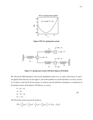
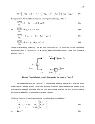
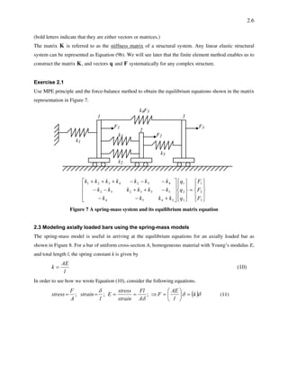
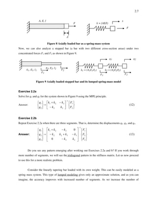
This document discusses the principle of minimum potential energy (MPE) and its application in finite element analysis of structures. MPE states that for conservative structural systems, the equilibrium state corresponds to the deformation that minimizes the total potential energy of the system. The document provides examples of applying MPE to simple spring-mass systems to derive equilibrium equations, and discusses how continuous systems can be approximated by discretizing them into lumped finite elements, allowing complex structures to be analyzed systematically using MPE.

1. Ananthasuresh, IISc
Chapter 2
The Principle of Minimum Potential Energy
The objective of this chapter is to explain the principle of minimum potential energy and its application in
the elastic analysis of structures. Two fundamental notions of the finite element method viz. discretization
and numerical approximation of the exact solution are also explained.
2.1 The principle of Minimum Potential Energy (MPE)
Deformation and stress analysis of structural systems can be accomplished using the principle of
Minimum Potential Energy (MPE), which states that
For conservative structural systems, of all the kinematically admissible deformations, those
corresponding to the equilibrium state extremize (i.e., minimize or maximize) the total potential
energy. If the extremum is a minimum, the equilibrium state is stable.
Let us first understand what each term in the above statement means and then explain how this principle
is useful to us.
A constrained structural system, i.e., a structure that is fixed at some portions, will deform when
forces are applied on it. Deformation of a structural system refers to the incremental change to the new
deformed state from the original undeformed state. The deformation is the principal unknown in structural
analysis as the strains depend upon the deformation, and the stresses are in turn dependent on the strains.
Therefore, our sole objective is to determine the deformation. The deformed state a structure attains upon
the application of forces is the equilibrium state of a structural system. The Potential energy (PE) of a
structural system is defined as the sum of the strain energy (SE) and the work potential (WP).
WPSEPE += (1)
The strain energy is the elastic energy stored in deformed structure. It is computed by integrating the
strain energy density (i.e., strain energy per unit volume) over the entire volume of the structure.
∫=
V
dVdensityenergystrainSE )( (2)
The strain energy density is given by
))((
2
1
strainstressdensityenergyStrain = (2a)

2. 2.2
The work potential WP, is the negative of the work done by the external forces acting on the structure.
Work done by the external forces is simply the forces multiplied by the displacements at the points of
application of forces. Thus, given a deformation of a structure, if we can write down the strains and
stresses, we can obtain SE, WP, and finally PE. For a structure, many deformations are possible. For
instance, consider the pinned-pinned beam shown in Figure 1a. It can attain many deformed states as
shown in Figure 1b. But, for a given force it will only attain a unique deformation to achieve equilibrium
as shown in Figure 1c. What the principle of MPE implies is that this unique deformation corresponds to
the extremum value of the MPE. In other words, in order to determine the equilibrium deformation, we
have to extremize the PE. The extremum can be either a minimum or a maximum. When it is a minimum,
the equilibrium state is said to be stable. The other two cases are shown in Figure 2 with the help of the
classic example of a rolling ball on a surface.
(a) (b) (c)
Figure 1 The notion of equilibrium deformed state of a pinned-pinned beam
Stable Unstable Neutrally stable
Figure 2 Three equilibrium states of a rolling ball
There are two more new terms in the statement of the principle of MPE that we have not touched upon.
They are conservative system and the kinematically admissible deformations. Conservative systems are
those in which WP is independent of the path taken from the original state to the deformed state.
Kinematically admissible deformations are those deformations that satisfy the geometric (kinematic)
boundary conditions on the structure. In the beam example above (see Figure 1), the boundary conditions
include zero displacement at either end of the beam. Now that we have defined all the terms in the
statement, it is a good time to read it again to make more sense out of it before we apply it.
2.2 Application of MPE principle to lumped-parameter uniaxial structural systems

3. 2.3
Consider the simplest model of an elastic structure viz. a mass suspended by a linear spring shown in
Figure 3. We would like to find the static equilibrium position of the mass when a force F is applied. We
will first use the familiar force-balance method, which gives
kxforcespringF == at equilibrium ( k is the spring constant)
∴
k
F
x mequilibriu == δ (3)
x
δ
F
Figure 3 Simplest model of an elastic structural system
We can arrive at the same result by using the MPE principle instead of the force-balance method. Let us
first write the PE for this system.
( ) FxkxFxkxWPSEPE −=−+⎟
⎠
⎞
⎜
⎝
⎛
=+= 22
2
1
2
1
)()( (4)
As per the MPE principle, we have to find the value of x that extremizes PE. The condition for
extremizing PE is that the first derivative of PE with respect to x is zero.
k
F
xFkx
dx
PEd
mequilibriu ==⇒=−⇒= δ00
)(
(5)
We got the same result as in Equation (3). Further, verify that the second derivative of PE with respect to
x is positive in this case. This means that the extremum is a minimum and therefore the equilibrium is
stable.
Figure 4 pictorially illustrates the MPE principle: of all possible deformations (i.e., the values of x
here), the stable equilibrium state corresponds to that x which minimizes PE. For the assumed values of k
= 5, and F = 10, equilibrium deflection is 2 which is consistent with Figure 4. As illustrated in Figure 3,
the MPE principle is an alternative way to write the equilibrium equations for elastic systems. It is, as we
will see, more efficient than the force-balance method. Let us now consider a second example of a spring-
mass system with three degrees of freedom viz. q1, q2, and q3. The number of degrees of freedom of a
system refers to the minimum number of independent scalar quantities required to completely specify the
system. It is easy to see that the system shown in Figure 5 has three degrees of freedom because we can
independently move the three masses to describe this completely.

4. 2.4
0 2 4
-10
-5
0
5
10
PE of a spring-mass system
x
PE
k = 5 and F = 10
Figure 4 PE of a spring-mass system
q1
F1
q3
q2
k1
k2
k3
k4
1
2
3
Figure 5 A spring-mass system with three degrees of freedom
We will use the MPE principle to solve for the equilibrium values of q1, q2, and q3 when forces F1 and F3
are applied (Note that one can also apply F2, but in this problem we assume that there is no force on mass
2). In order to write the SE for the springs, we need to write the deflection (elongation or contraction) of
the springs in terms of the degrees of freedom q1, q2, and q3.
34
233
22
211
qu
qqu
qu
qqu
−=
−=
=
−=
(6)
The PE for this system can now be written as
( )3311
2
44
2
33
2
22
2
11
2
1
2
1
2
1
2
1
qFqFukukukukPE −−+⎟
⎠
⎞
⎜
⎝
⎛
+++=

5. 2.5
( ) ( ) ( )3311
2
34
2
233
2
22
2
211
2
1
2
1
2
1
2
1
qFqFqkqqkqkqqkPE −−+⎟
⎠
⎞
⎜
⎝
⎛
+−++−= (7)
For equilibrium, PE should be an extremum with respect to all three q’s. That is,
0
)(
=
∂
∂
iq
PE
for i = 1, 2, and 3. (8a)
i.e., 0)(
)(
1211
1
=−−=
∂
∂
Fqqk
q
PE
(8b)
0)()(
)(
23322211
2
=−−+−−=
∂
∂
qqkqkqqk
q
PE
(8c)
0)(
)(
334233
3
=−+−=
∂
∂
Fqkqqk
q
PE
(8d)
Noting the relationship between q’s and u’s from Equation (6), we can readily see that the equilibrium
equations obtained in Equations (8) can be directly obtained from force-balance on the three masses as
shown in Figure 6.
F1
k1 u1
k2 u2
1
2
3
k1 u1
k3 u3 k3 u3
k4 u4
Figure 6 Force-balance free-body-diagrams for the system in Figure 5
It is important to note that Equations (8) were obtained routinely from the MPE principle where
as force-balance method requires careful thinking about the various forces (including the internal spring
reaction forces and their directions. Thus, for large and complex systems, the MPE method is clearly
advantageous, especially for implementation on the computer.
The linear Equations (8) can be written in the form of matrix system as follows:
⎪
⎭
⎪
⎬
⎫
⎪
⎩
⎪
⎨
⎧
=
⎪
⎭
⎪
⎬
⎫
⎪
⎩
⎪
⎨
⎧
⎥
⎥
⎥
⎦
⎤
⎢
⎢
⎢
⎣
⎡
+−
−++−
−
3
1
3
2
1
433
33211
11
0
0
0
F
F
q
q
q
kkk
kkkkk
kk
(9a)
or FKq = (9b)

6. 2.6
(bold letters indicate that they are either vectors or matrices.)
The matrix K is referred to as the stiffness matrix of a structural system. Any linear elastic structural
system can be represented as Equation (9b). We will see later that the finite element method enables us to
construct the matrix K, and vectors q and F systematically for any complex structure.
Exercise 2.1
Use MPE principle and the force-balance method to obtain the equilibrium equations shown in the matrix
representation in Figure 7.
F3
1
2
3
k1
k2
k3
k4
k5
F3
F2
F1
⎪
⎭
⎪
⎬
⎫
⎪
⎩
⎪
⎨
⎧
=
⎪
⎭
⎪
⎬
⎫
⎪
⎩
⎪
⎨
⎧
⎥
⎥
⎥
⎦
⎤
⎢
⎢
⎢
⎣
⎡
+−−
−++−−
−−−+++
3
2
1
3
2
1
5454
553232
4324321
F
F
F
q
q
q
kkkk
kkkkkk
kkkkkkk
Figure 7 A spring-mass system and its equilibrium matrix equation
2.3 Modeling axially loaded bars using the spring-mass models
The spring-mass model is useful in arriving at the equilibrium equations for an axially loaded bar as
shown in Figure 8. For a bar of uniform cross-section A, homogeneous material with Young’s modulus E,
and total length l, the spring constant k is given by
l
AE
k = (10)
In order to see how we wrote Equation (10), consider the following equations.
( )δδ
δ
δ
k
l
AE
F
A
Fl
strain
stress
E
l
strain
A
F
stress =⎟
⎠
⎞
⎜
⎝
⎛
=⇒==== ;;; (11)

7. 2.7
x
δ
F
F
A, E, l
k = (AE/l)
Figure 8 Axially loaded bar as a spring-mass system
Now, we can also analyze a stepped bar (a bar with two different cross-section areas) under two
concentrated forces F1 and F2 as shown in Figure 9.
q1
A1, E1, l1 k1 = (A1E1/l1)F2
F1
A2, E2, l2
k2 = (A2E2/l2)
q2
F1 F2
Figure 9 Axially loaded stepped bar and its lumped spring-mass model
Exercise 2.2a
Solve for q1 and q2 for the system shown in Figure 9 using the MPE principle.
Answer:
⎭
⎬
⎫
⎩
⎨
⎧
⎥
⎦
⎤
⎢
⎣
⎡
−
−+
=
⎭
⎬
⎫
⎩
⎨
⎧
−
2
1
1
22
221
2
1
F
F
kk
kkk
q
q
(12)
Exercise 2.2b
Repeat Exercise 2.2a when there are three segments. That is, determine the displacements q1, q2, and q3.
Answer:
⎪
⎭
⎪
⎬
⎫
⎪
⎩
⎪
⎨
⎧
⎥
⎥
⎥
⎦
⎤
⎢
⎢
⎢
⎣
⎡
−
−+−
−+
=
⎪
⎭
⎪
⎬
⎫
⎪
⎩
⎪
⎨
⎧
−
3
2
1
1
33
3322
221
3
2
1
0
0
F
F
F
kk
kkkk
kkk
q
q
q
(13)
Do you see any pattern emerging after working out Exercises 2.2a and b? If you work through
more number of segments, we will see the tridiagonal pattern in the stiffness matrix. Let us now proceed
to use this for a more realistic problem.
Consider the linearly tapering bar loaded with its own weight. This can be easily modeled as a
spring mass system. This type of lumped modeling gives only an approximate solution, and as you can
imagine, the accuracy improves with increased number of segments. As we increase the number of

8. 2.8
segments, the number of degrees of freedom increases (i.e., more q’s) and the size of the stiffness matrix
increases. But, the procedures for doing two bar segments in Figure 9 or many bar segments in Figure 10
are exactly the same, except that it is repetitive and tedious as the number of segments increases.
However, it is ideal for implementation on a computer. Notice that k for each segment is of the identical
form.
...
Tapering bar loaded
with its own weight
A lumped model
Figure 10 A tapering bar loaded with its own weight, and its lumped spring-mass model
This example illustrates two important concepts.
• Continuous systems can be approximated as lumped segments. This is called discretization⎯an
important concept in FEM. The segments are called “finite elements”.
• All elements have the identical form. So, a general method can be developed to handle large
and complex structures. That is, by discretizing the structure into identical elements, the whole
structure can be analyzed in a repetitive manner systematically.
What we have done in this Chapter is not FEM yet. It suffices to note at this point that FEM
provides a systematic way of discretizing a complex structure to get an approximate solution. In addition
to the intuitive notion presented in this chapter, there is a firm theoretical basis for FEM. We will examine

9. 2.9
that in the later Chapters. Before we embark upon FEM formulation, it is worthwhile to discuss another
important concept method called the Rayleigh-Ritz method. That is the topic of the next Chapter.
2.4 Implementation of mass-spring systems in Matlab
The finite element method is a numerical method. It is important to understand the practical
implementation of it in addition to gaining a theoretical understanding of it. This notes emphasizes this
aspect and includes finite element programs written in Matlab. You can do this in Maple, Mathematica,
MathCad or anything else you are comfortable with. In order to be prepared to handle the finite element
programs later, let us get started here with a simple Matlab script to solve the problem shown in Figure
11.
Exercise 2.3
Write down the matrix equation system for the system shown in Figure 11 and study its implementation
in the attached Matlab script. Run the script to get experience with Matlab.
850kN
650 kN
1500 kN
Aluminum bar
Brass tube
Steel pipe
The steel pipe ID and OD are 125 mm and 200 mm.
The brass tube ID and OD are 100 mm and 150 mm.
The aluminum bar cross-section diameter is 100 mm.
E-steel = 210 GPa
E-brass = 100 GPa
E-aluminum = 73 GPa
Find the displacements at the points where forces are applied.
Figure 11 A composite axially loaded system
____________________________________
Matlab script 1 for Exercise 2.3
clear all
clc
clg
hold off
axis normal
% Aluminum bar
E1 = 73E9; % Pa
A1 = (pi/4)*(100E-3)^2; % m^2
L1 = 1.0; % m

10. 2.10
% Brass tube
E2 = 100E9; % Pa
A2 = (pi/4)*( (150E-3)^2 - (100E-3)^2 ) ; % m^2
L2 = 1.25; % m
% Steel pipe
E3 = 210E9; % Pa
A3 = (pi/4)*( (200E-3)^2 - (125E-3)^2 ); % m^2
L3 = 0.75; % m
% Forces
F = [-650 -850 -1500]*1e3; % N
% Compute the spring constants
k1 = A1*E1/L1;
k2 = A2*E2/L2;
k3 = A3*E3/L3;
% Construct the stiffness matrix of the system
K(1,1) = k1;
K(1,2) = -k1;
K(1,3) = 0;
K(2,1) = -k1;
K(2,2) = k1+k2;
K(2,3) = -k2;
K(3,1) = 0;
K(3,2) = -k2;
K(3,3) = k2+k3;
% Solve for displacements
u = inv(K)*F'
____________________________________
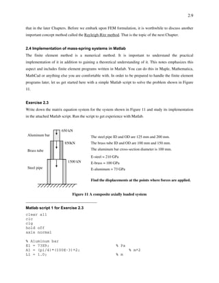
Exercise 2.4
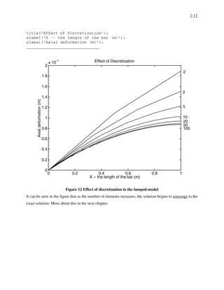
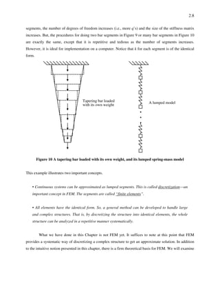
Solve the linearly tapering bar problem by using a Matlab script. The advantage of writing in Matlab (or
other similar software) is that we can vary the number of elements (i.e., the “fineness” of discretization)
and observe what happens. Assume the following data.
The bar is made of aluminum (E = 73 GPa, mass density = 2380 Kg/m3
), and has a circular cross-section
with beginning diameter of 100 mm and tip diameter of 20 mm. The length of the bar is 1 m.
____________________________________
Matlab script 2 for Exercise 2.4

11. 2.11
clear all
clc
%clg
%hold off
axis normal
% Tapering aluminum bar under its own weight
E = 73E9; % Pa
A0 = (pi/4)*(100E-3)^2; % m^2
At = (pi/4)*(20E-3)^2; % m^2
L = 1.0; % m
rho = 2380*9.81; % N/m^3
echo on
N = 2; % Number of elements
% Change the number of elements and see the how the accuracy
% of the solution improves. You need to run the script many
% times by changing the number of element N, above.
% Note that the hold on graphics is on.
echo off
% Compute element length, area, k and force
Le = L/N;
for i = 1:N,
Atop = A0 -(A0-At)/N*(i-1);
Abot = A0 - (A0-At)/N*i;
A(i) = (Atop+Abot)/2;
x(i) = L/N*i;
k(i) = A(i)*E/Le;
F(i) = A(i)*Le*rho;
end
% Assembly of the stiffness matrix using k's.
K = zeros(N,N);
K(1,1) = k(1) + k(2);
K(1,2) = -k(2);
for i = 2:N-1,
K(i,i-1) = -k(i);
K(i,i) = k(i) + k(i+1);
K(i,i+1) = -k(i+1);
end
K(N,N-1) = -k(N);
K(N,N) = k(N);
% Solve for displacements {q}. It is a column vector.
q = inv(K)*F';
plot([0 x],[0; q],'-w',x,q,'c.');
hold on

12. 2.12
title('Effect of Discretization');
xlabel('X -- the length of the bar (m)');
ylabel('Axial deformation (m)');
____________________________________
0 0.2 0.4 0.6 0.8 1
0
0.2
0.4
0.6
0.8
1
1.2
1.4
1.6
1.8
2
x 10-7 Effect of Discretization
X -- the length of the bar (m)
Axialdeformation(m)
2
3
5
10
20
50
100
Figure 12 Effect of discretization in the lumped-model
It can be seen in the figure that as the number of elements increases, the solution begins to converge to the
exact solution. More about this in the next chapter.