Downloaded 201 times
![Formation of filter equations for
PLL20
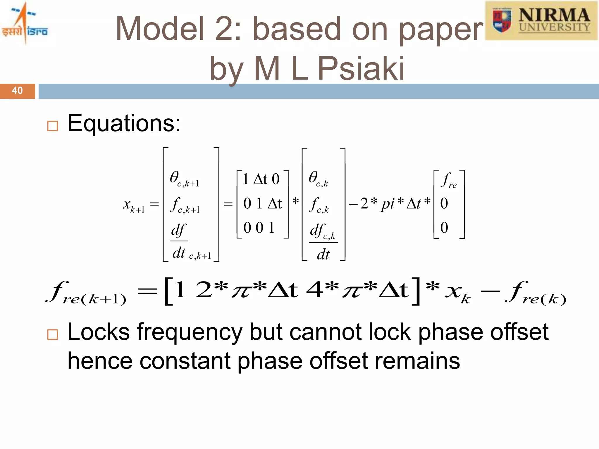
Phase difference and frequency difference
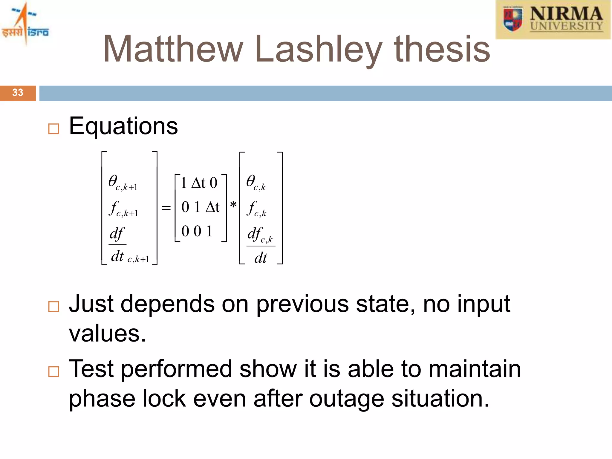
were selected to be the parameters for state
equations
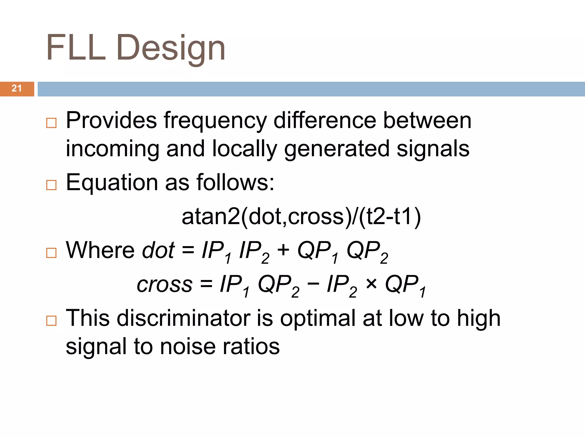
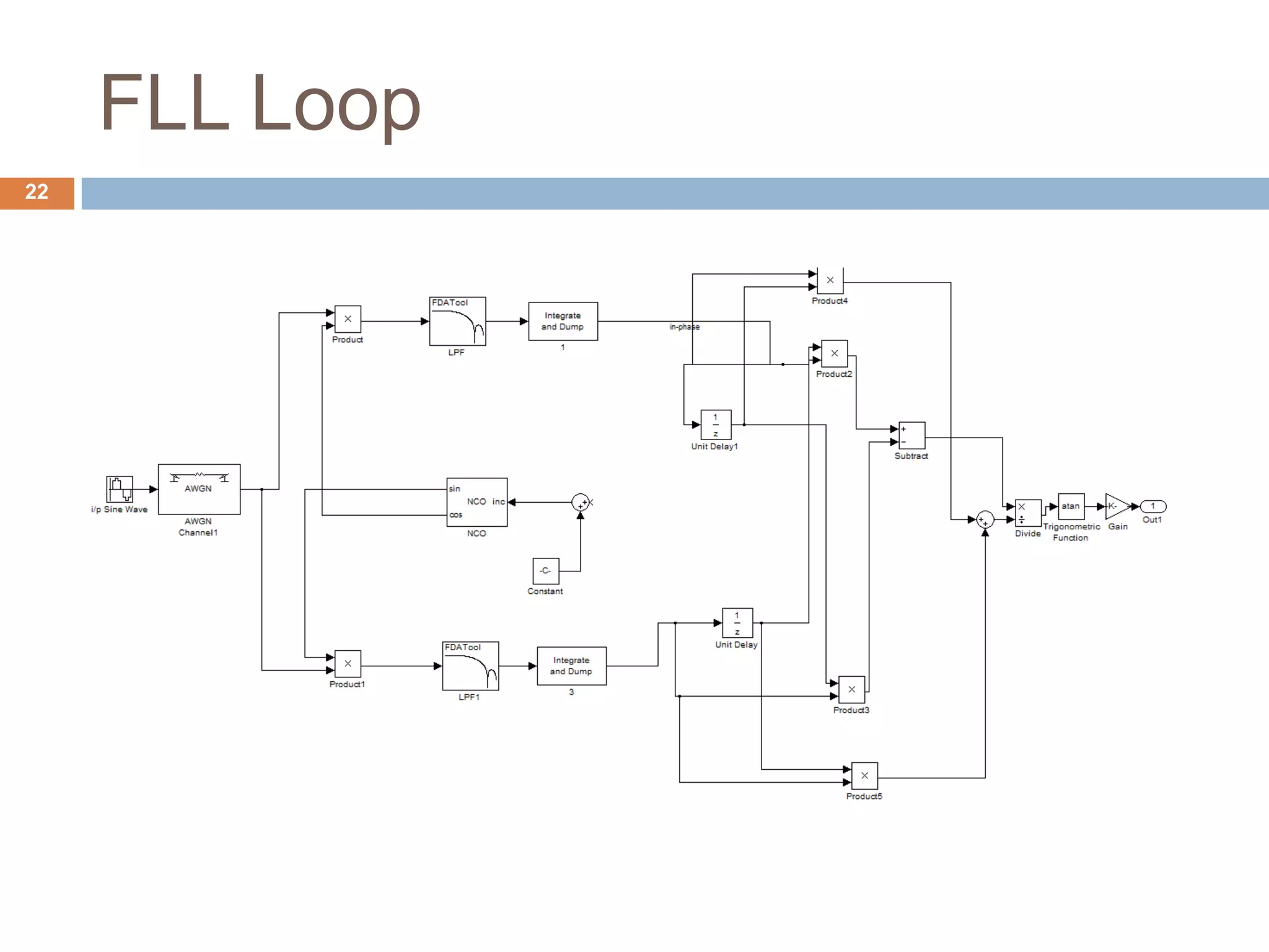
Requirements: Design of FLL, error variance
in measurement of phase and frequency
Deciding the control inputs for the state
equations
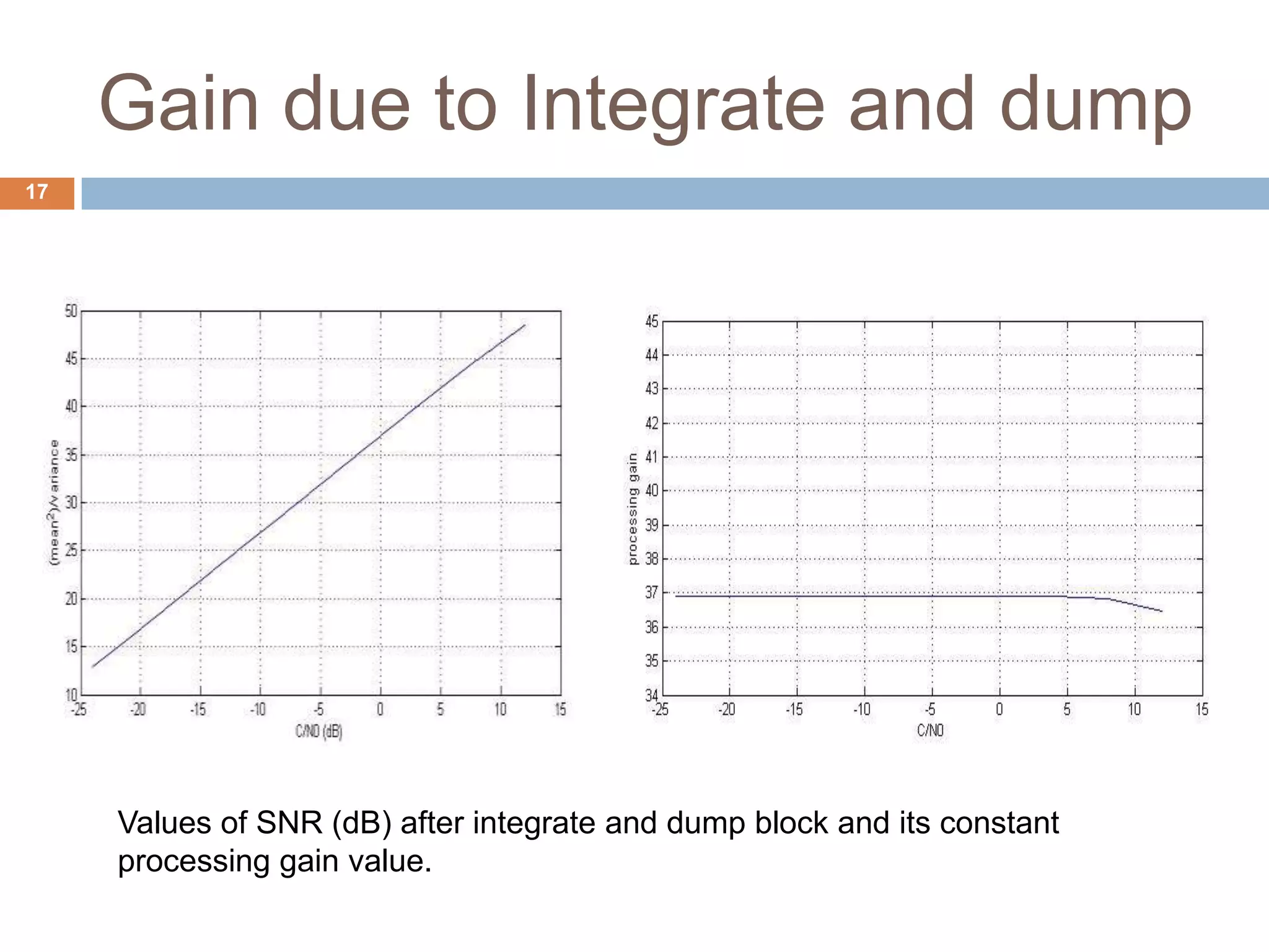
Finding variance for different values of C/N0
which are 40 dB-Hz to 80 dB-Hz for GPS
signals
Measurement matrix becomes [1 2*pi*T ;0 1]
](https://image.slidesharecdn.com/majorprojectppt-140322125718-phpapp01/75/Kalman-Filter-Based-GPS-Receiver-20-2048.jpg)
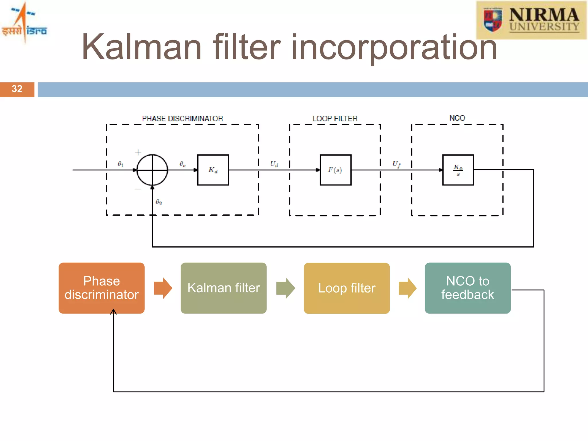
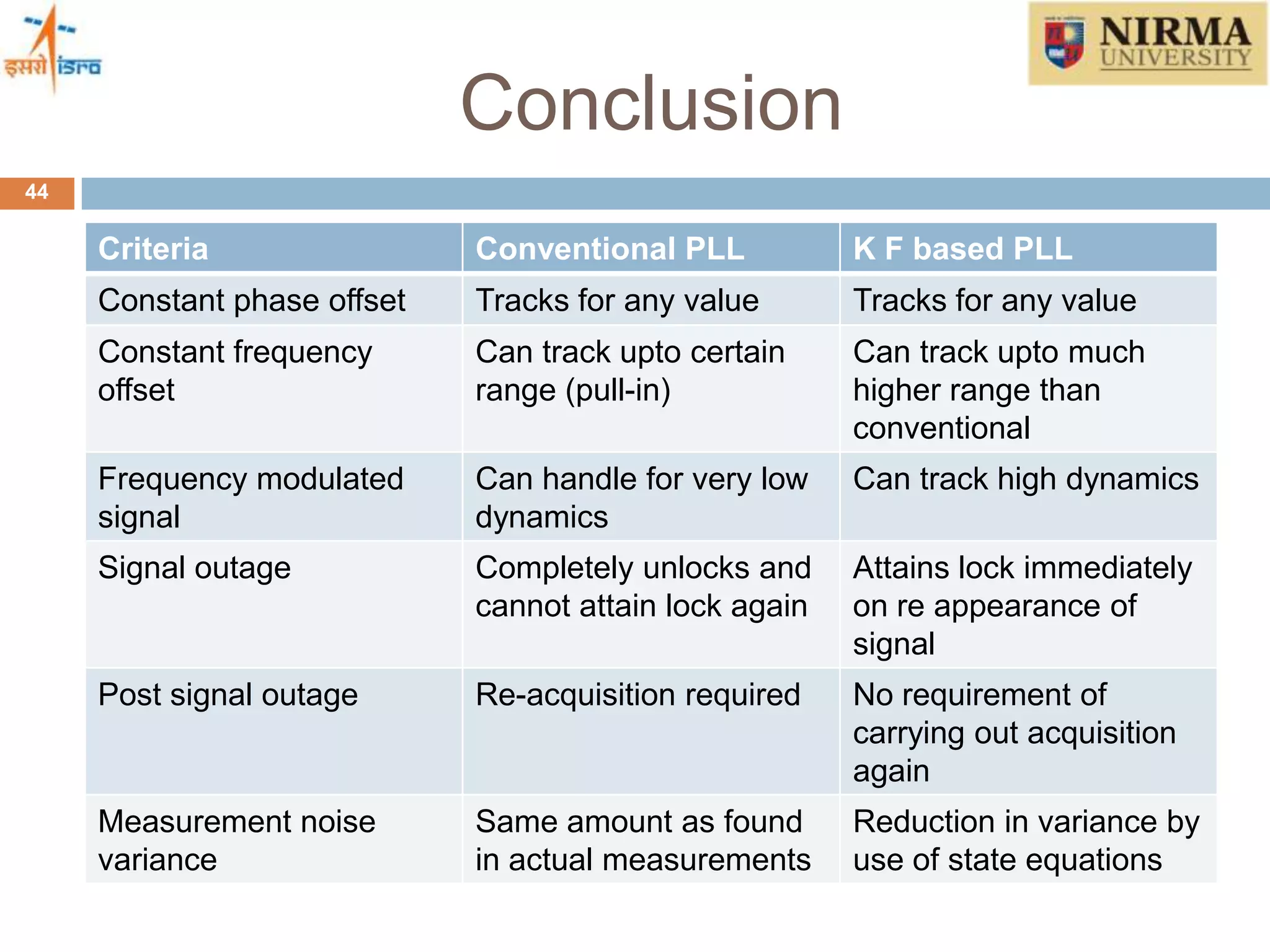


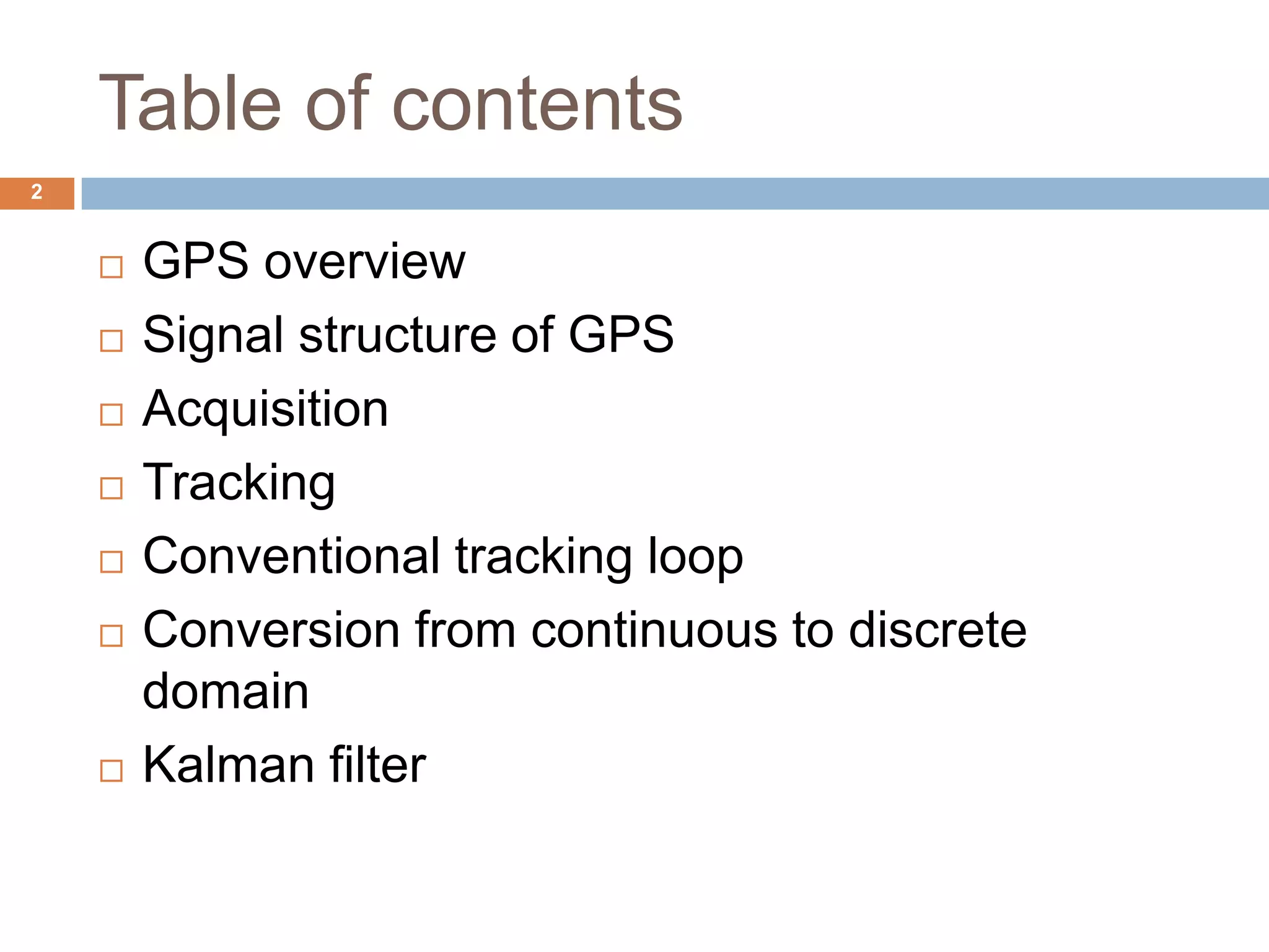
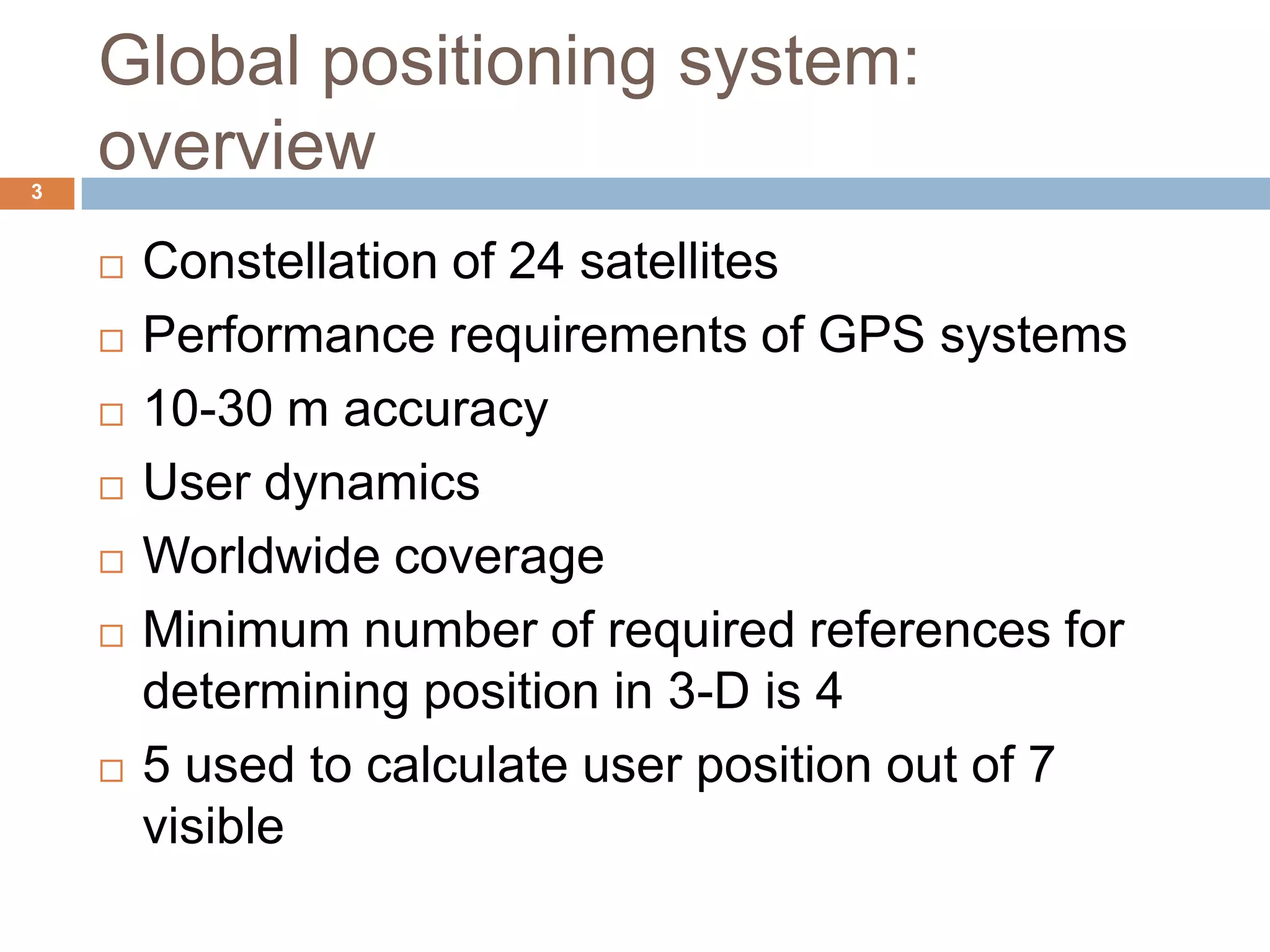
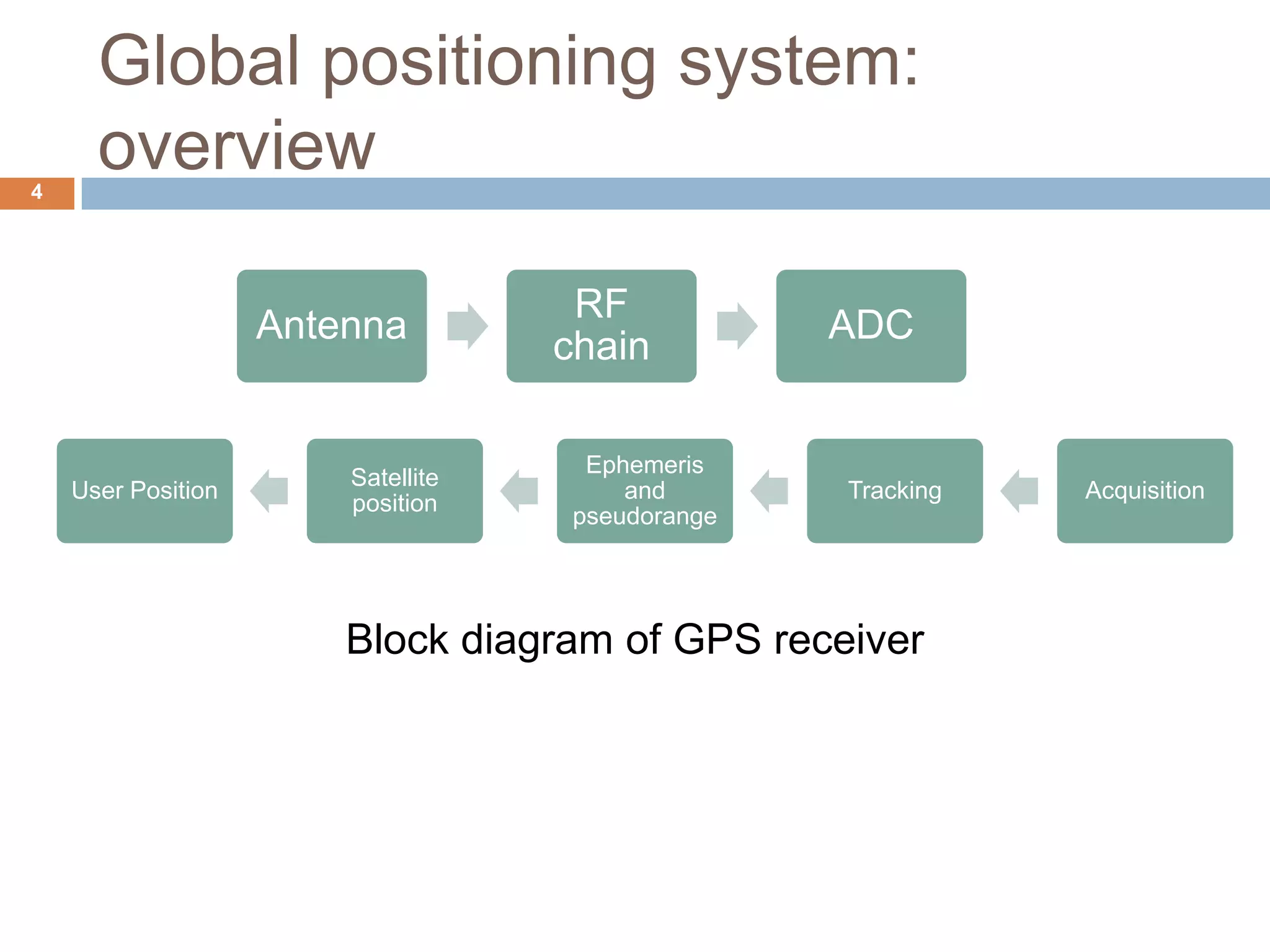
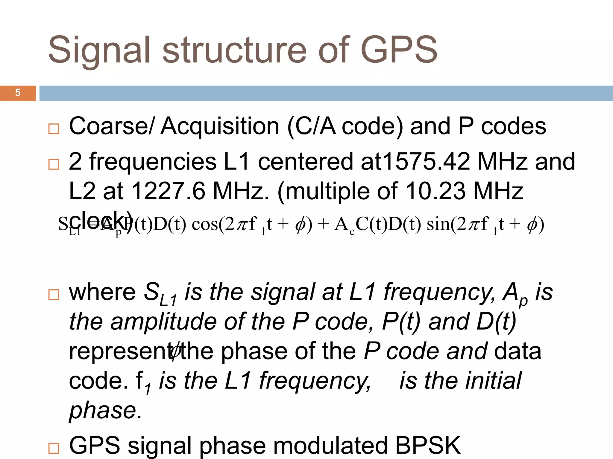
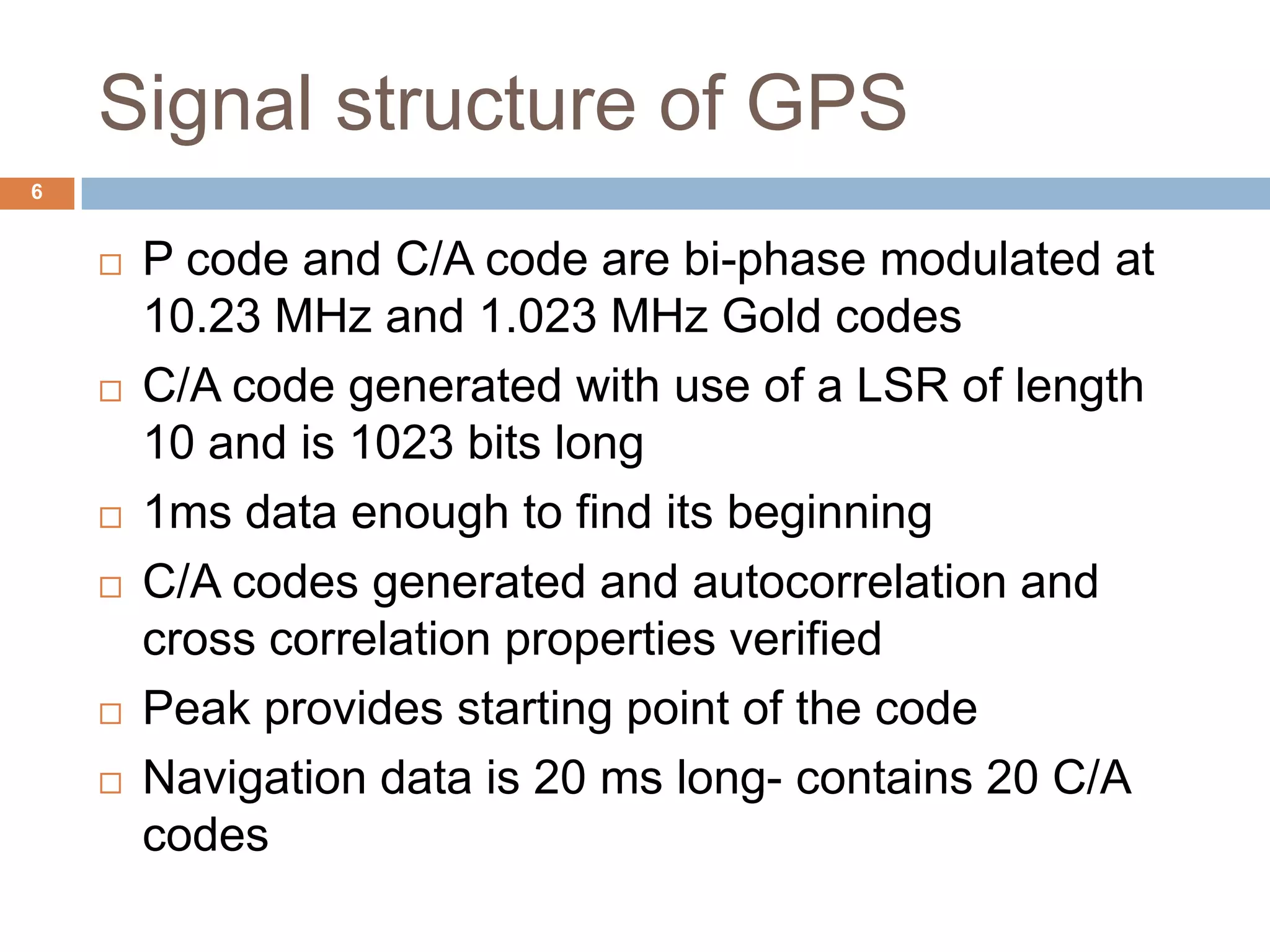
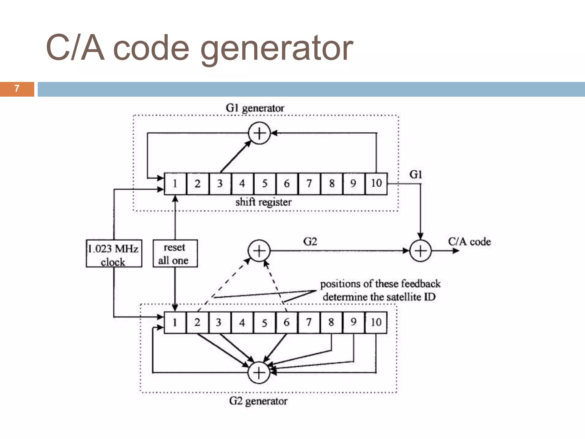
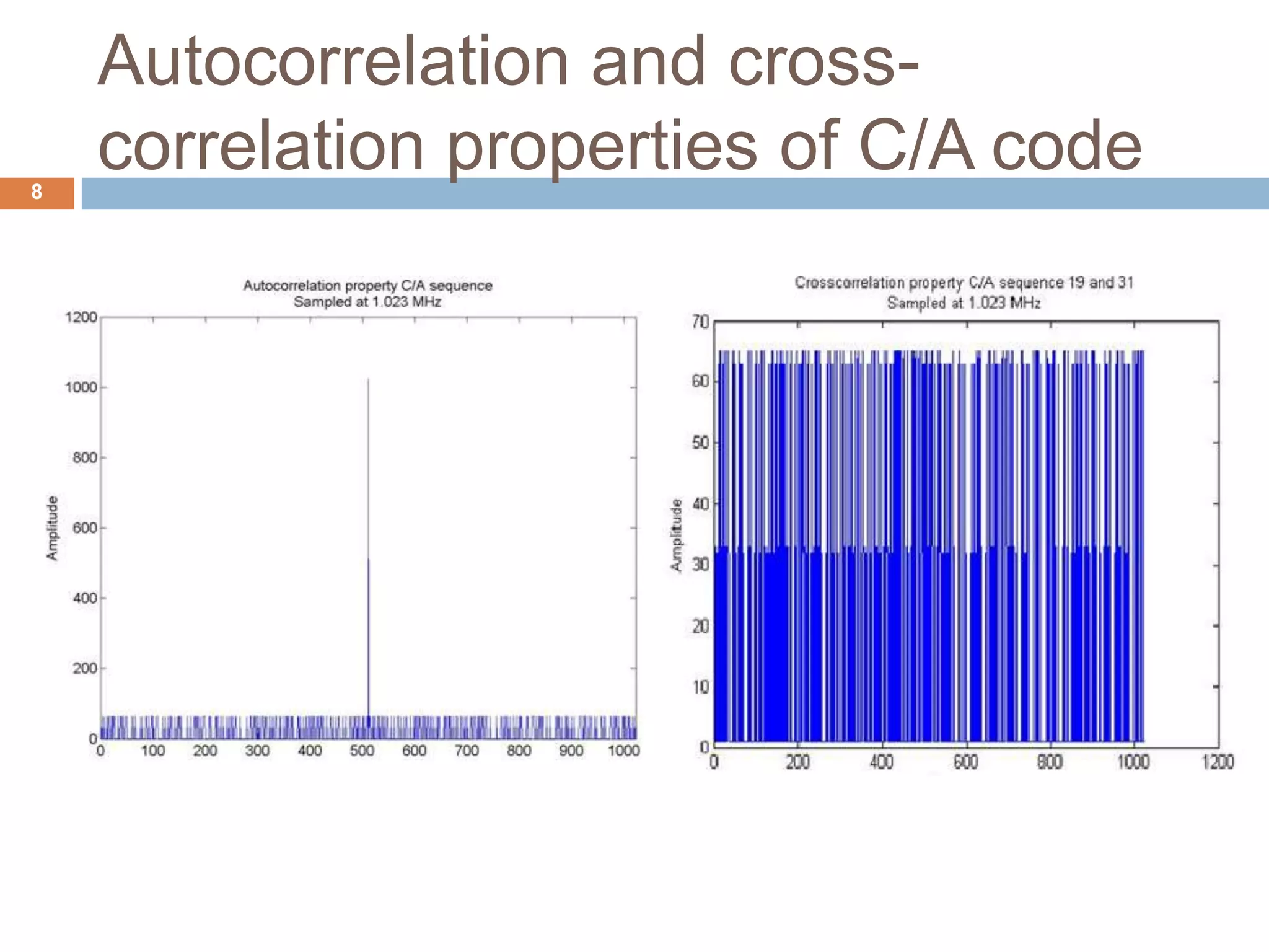
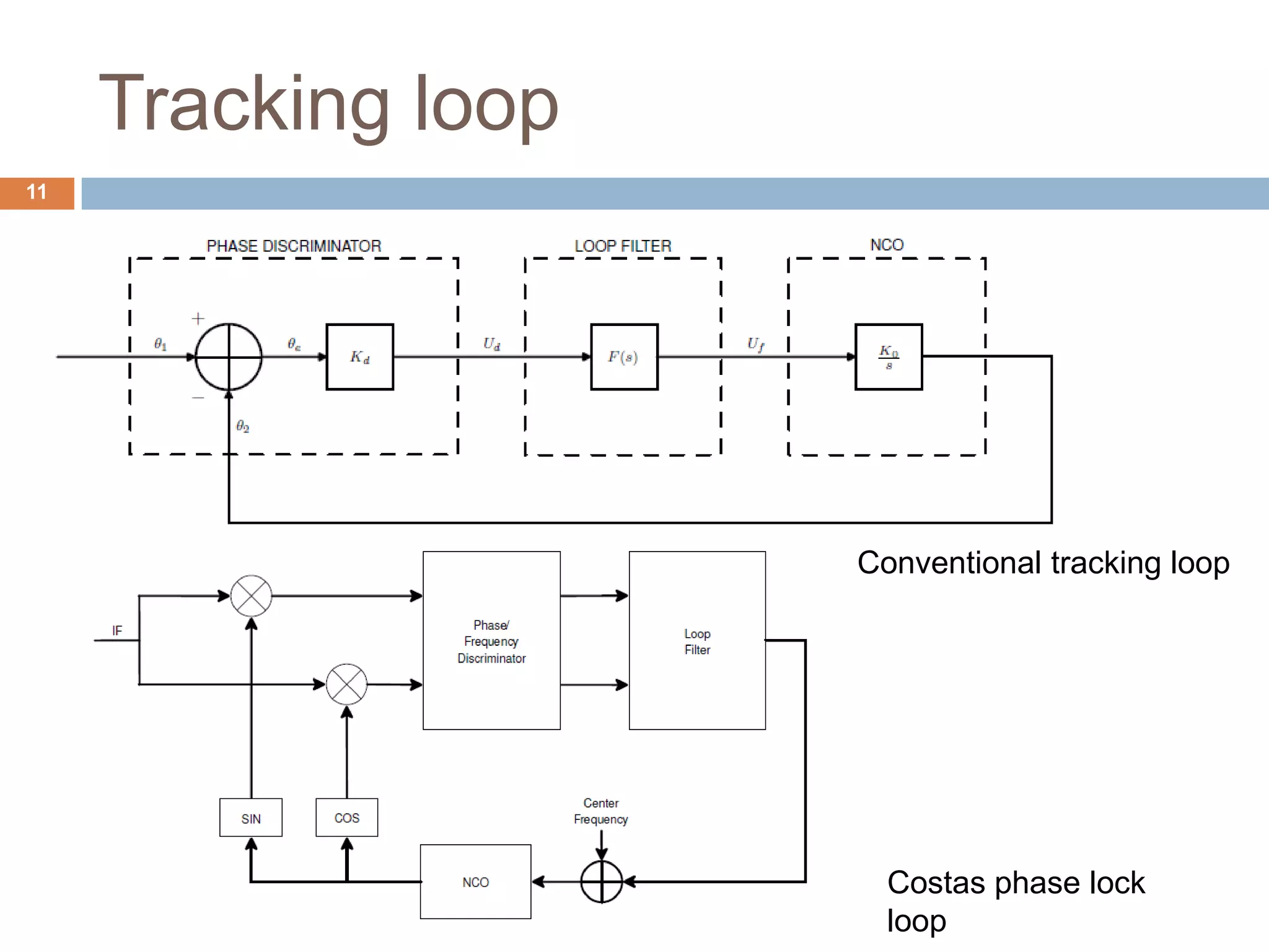
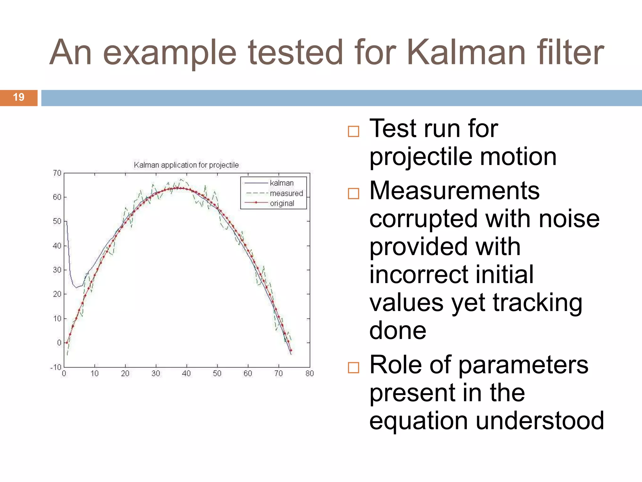
This document provides an overview of Kalman filter based GPS tracking. It discusses: 1) The basics of GPS including its satellite constellation and accuracy requirements. 2) The signal structure of GPS including the C/A and P codes transmitted on two frequencies. 3) How a conventional tracking loop works and its limitations in high dynamic situations. 4) How a Kalman filter can be incorporated into the tracking loop to optimally estimate GPS signals and overcome the limitations of conventional tracking loops. Simulation results show the Kalman filter based approach can track signals in high dynamics and during brief signal outages.