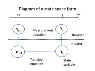
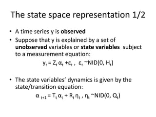
This document provides an overview of forecasting and smoothing using the Kalman filter. It discusses (1) how state space models represent time series using unobserved state variables, (2) how the Kalman filter recursively estimates the state variables using past and current observations, and (3) how maximum likelihood estimation and forecasting/smoothing techniques utilize the Kalman filter outputs. The document uses examples from macroeconomic forecasting to illustrate these concepts.

1. Forecasting and Smoothing using
the Kalman Filter
Macroeconomic Forecasting
Reda Cherif
This training material is the property of the International Monetary Fund (IMF) and is
intended for use in IMF Institute for Capacity Development courses. Any reuse
requires the permission of the IMF Institute for Capacity Development.

2. Roadmap
I. Introduction
II. The state space representation
III. The Kalman filter
IV. ML estimation and the Kalman filter
V. Forecasting and smoothing
VI. Concluding remarks
This training material is the property of the International Monetary Fund (IMF) and is intended
for use in IMF Institute courses. Any reuse requires the permission of the IMF Institute.”

3. I. Introduction
• The dynamics of time series could be influenced
by the dynamics of a set of variables i.e. states.
• State space models describe the law of motion of
the states and their link with observations. The
Kalman filter is an algorithm to estimate it.
• Classical regression analysis would fail in terms of
validity of tests (t-test F-test…) and in terms of
forecasts if these states were unobservable and
persistent.
• State space representation encompasses the
standard models (e.g. ARMA).

4. II. State Space Representation

5. Yt
time
t-1 t
Yt-1
Observed
Hidden
Diagram of a state space form
αt-1 αt
Transition
equation
Measurement
equation
State
variable

6. The state space representation 1/2
• A time series y is observed
• Suppose that y is explained by a set of
unobserved variables or state variables subject
to a measurement equation:
yt = Zt αt +εt , εt ~NID(0, Ht)
• The state variables’ dynamics is given by the
state/transition equation:
α t+1 = Tt αt + Rt ηt , ηt ~NID(0, Qt)

7. The state space representation 2/2
• It is also assumed that:
E(εt ηs)=0, E(α0 εt)=0 and E(α0 ηt)=0
• The model can also include exogenous
variables both in the measurement and
transition equations.

8. Hyper-Parameters
• In the state space model the parameters Ht Qt
Rt Tt Zt are referred to as “hyper-parameters”
and are unknown in general.
• The main task of the Kalman filter will be to
estimate these parameters.
• Contrary to standard regressions, there are no
analytical solutions and the estimation
requires an iterative procedure (maximum
likelihood).

9. Why a recursive algorithm is the
natural approach to state space forms?
• In a state space form the notion of forecasting
given different information sets appears naturally
(e.g. dynamic vs. one-step-ahead).
• Given information on the initial state (time t), it is
possible to construct a forecast of the state (time
t+1).
• Given the observation (time t+1), it is possible to
refine the estimate of the state (time t+1).
• Given initial conditions, the recursion could be
used for the estimation.

10. III. The Kalman filter

11. Filtering, predicting and smoothing?
• All these refer to the same concept i.e.
estimating the state vector.
• The difference between them is the set of
information used in the estimate:
 Filtering is based on past observations and current
observations.
 Predicting is based on past observations only.
 Smoothing is based on all past and future
observations.

12. The Kalman filter
• The Kalman filter is a recursive procedure to
estimate the state vector of a state space form
given all past and current observations.
• Given an initial state vector (normality) and
hyper-parameters or transition matrices, the
Kalman filter computes recursively the
conditional distributions of the state vector.
• It has applications in engineering e.g. satellite
location.

13. Properties of the Kalman filter
• Under normality condition (initial state and
disturbances), the Kalman filter produces an
optimal estimator of the state vector
(minimum Mean Square Error).
• If normality is dropped the Kalman filter still
produces the optimal estimator in the class of
linear predictors.

14. Algorithm: schematic diagram
Kalman
filtered
state: at
Predicted
state:
at+1|t=Ttat
Predicted
observation:
yt+1|t=Ztat+1|t
yt+1 is observed
Forecast error:
vt = yt+1 - yt+1|t
Kalman gain: Kt
Kalman filtered
state:
at+1=at+1|t+Ktvt
time
t+1
t

15. Initialization
• The starting value of the Kalman filter may be
specified in terms of a0 and P0
• Diffuse initialization means that the initial
values are estimated
• They can be measured from outside
information.

16. Period t: initial values
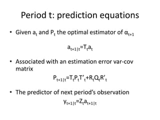
• Let at denote the optimal estimator of αt the
state vector at time t given all past
information including yt i.e. the Kalman
filtered state.
• Let Pt denote var-cov of the estimation error:
Pt=E[(αt- at) (αt- at)’]

17. Period t: prediction equations
• Given at and Pt the optimal estimator of αt+1
at+1|t=Ttat
• Associated with an estimation error var-cov
matrix
Pt+1|t=TtPtT’t+RtQtR’t
• The predictor of next period’s observation
yt+1|t=Ztat+1|t

18. Period t+1: Forecasting error
• Observing yt+1 yields the forecast error:
vt = yt+1 - yt+1|t
• Associated with the var-covar matrix:
Ft =ZtPt+1|tZ’t+Ht
• Define the Kalman gain:
Kt =Pt+1|tZ’t Ft
-1

19. Period t+1: Updating equations
• Given the forecast error, the Kalman filtered
state at time t+1 is an update of at+1|t:
at+1=at+1|t+Ktvt
• Associated with the var-covar matrix:
Pt+1 =Pt+1|t-KtZtPt+1|t

20. The Kalman gain and updating
• The Kalman gain measures the uncertainty of
the state based on past observations relative
to the uncertainty of the new observation.
• It determines the influence of the prediction
error of yt+1|t on the estimate of the state at
time t+1.
• In time-invariant models the Kalman gain
converges to a constant simplifying the
calculation of steady-state Kalman filter.

21. GPS and Kalman?

22. An Application of Kalman filtering

23. IV. ML estimation

24. Estimation
• The Kalman filter is applied given the hyper-
parameters. But how do we estimate those?
• The Kalman filter plays a crucial role in their
estimation too! Why?
• The reason stems from the way the Likelihood
function is calculated.

25. Maximum likelihood
• The theory of ML: given a set of observations
y=y1 ,…, yT (iid):
L(y,Ψ)=p(y1)…p(yT)
• In the state space model the observations are
not iid, thus instead:
L(y,Ψ)=Πp(yt|yt-1,yt-2,…,y1)
• Under normality conditions (initial state and
disturbances) yt|yt-1,yt-2,…,y1~N

26. ML and the Kalman filter
• The Kalman filter computes the mean and covariance
of yt|yt-1,yt-2,…,y1
• The mean is Ztat and the variance is Ft
• Numerical techniques yield the ML estimator of hyper-
parameters Ψ
• In the univariate model the log lieklihood is:
-T/2log(2π)-1/2(logF1+ v1
2 /F1+…+logFT+ vT
2 /FT)
• The maximization is such that the weight on past
observations minimizes the prediction error of current
observation (unlike classical regressions where past
and future have the same weight).

27. V. Forecasting and smoothing

28. Forecasting
• A state space form is estimated (suppose time
invariant).
• Suppose the last observation occurs at T+1.
• The filtered state at time T+1 is updated:
aT+1=aT+1|T+KTvT
• The forecast for T+n is simply:
yT+n|T=Z(T)n-1 aT+1

29. Smoothing
• Recursive algorithms “state and disturbance
smoothers” are applied to the output of the
Kalman filter.
• The goal is to obtain an estimate of the state
vector taking into account all observations
(past and future).
• Could be applied to estimate potential GDP
for example.

30. VI. Concluding remarks
• The state space model/Kalman filter is a
powerful and flexible tool. It can be applied to
non-stationary time series.
• It handles difficult issues like time varying
coefficients and missing data relatively easily.
• The normality condition is important to
ensure optimality and there are methods to
verify it.