Downloaded 278 times

![ASU-CSC445: Neural Networks Prof. Dr. Mostafa Gadal-Haqq
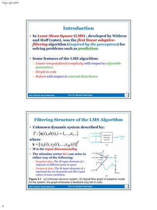
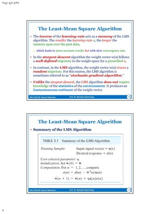
Filtering Structure of the LMS Algorithm
Unknown dynamic system described by:
Figure 3.1 (a) Unknown dynamic system. (b) Signal-flow graph of adaptive model
for the system; the graph embodies a feedback loop set in color.
4
T
M ixixix )](),...,(),([ 21x
,...,...,1),(),(: niidiΤ x
where
M is the input dimensionality
The stimulus vector x(i) can arise in
either way of the following:
Snapshot data, The M input elements of x
originate at different point in space
Temporal data, The M input elements of x
represent the set of present and (M-1) past
values of some excitation.](https://image.slidesharecdn.com/fiwxhftptkf6j4yed2ee-signature-7f7e9932c1ac6134e9030bbdd4cfa1c5606f58d572ef5d7da58609957cc1fc67-poli-160617131027/85/Neural-Networks-Least-Mean-Square-LSM-Algorithm-4-320.jpg)
![ASU-CSC445: Neural Networks Prof. Dr. Mostafa Gadal-Haqq
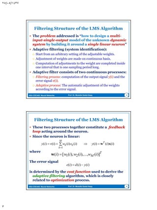
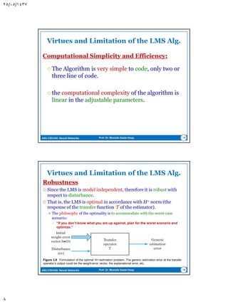
Filtering Structure of the LMS Algorithm
These two processes together constitute a feedback
loop acting around the neuron.
Since the neuron is linear:
where
The error signal
is determined by the cost function used to derive the
adaptive-filtering algorithm, which is closely
related to optimization process.
6
)()()()()()()(
1
iiiyixiwiviy T
M
k
kk xw
T
M iwiwiwi )](),...,(),([)( 21w
)()()( iyidie ](https://image.slidesharecdn.com/fiwxhftptkf6j4yed2ee-signature-7f7e9932c1ac6134e9030bbdd4cfa1c5606f58d572ef5d7da58609957cc1fc67-poli-160617131027/85/Neural-Networks-Least-Mean-Square-LSM-Algorithm-6-320.jpg)


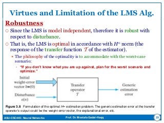
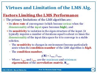
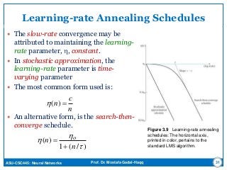


The document discusses the Least-Mean Square (LMS) algorithm. It begins by introducing LMS as the first linear adaptive filtering algorithm developed by Widrow and Hoff in 1960. It then describes the filtering structure of LMS, modeling an unknown dynamic system using a linear neuron model and adjusting weights based on an error signal. Finally, it summarizes the LMS algorithm, outlines its virtues like computational simplicity and robustness, and notes its primary limitation is slow convergence for high-dimensional problems.


