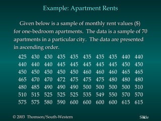
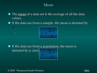
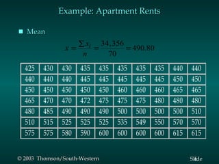
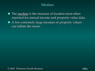
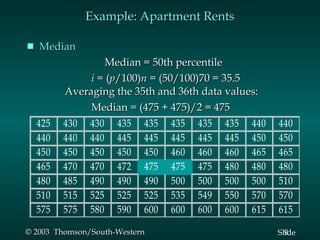
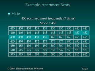
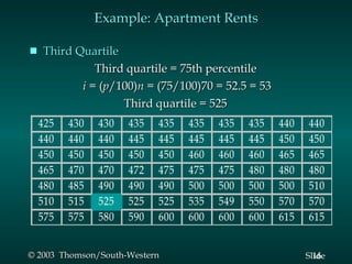
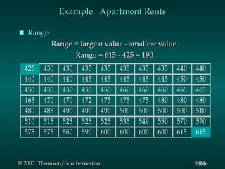
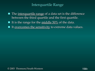
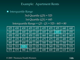
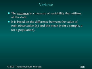
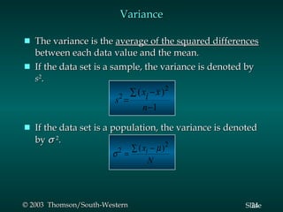
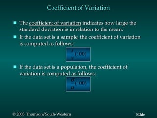
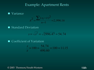
Slides Prepared by JOHN S. LOUCKS St. Edward’s University
Chapter 3  Descriptive Statistics:  Numerical Methods Part A Measures of Location Measures of Variability x   %
Measures of Location Mean Median Mode Percentiles Quartiles
Example: Apartment Rents Given below is a sample of monthly rent values ($) for one-bedroom apartments.  The data is a sample of 70 apartments in a particular city.  The data are presented in ascending order.
Mean The  mean  of a data set is the average of all the data values. If the data are from a sample, the mean is denoted by  . If the data are from a population, the mean is denoted by     (mu).
Example: Apartment Rents Mean
Median The  median  is the measure of location most often reported for annual income and property value data. A few extremely large incomes or property values can inflate the mean.
Median The  median  of a data set is the value in the middle when the data items are arranged in ascending order. For an odd number of observations, the median is the middle value. For an even number of observations, the median is the average of the two middle values.
Example: Apartment Rents Median   Median = 50th percentile i  = ( p /100) n  = (50/100)70 = 35.5     Averaging the 35th and 36th data values: Median = (475 + 475)/2 = 475
Mode The  mode  of a data set is the value that occurs with greatest frequency. The greatest frequency can occur at two or more different values. If the data have exactly two modes, the data are  bimodal . If the data have more than two modes, the data are  multimodal .
Example: Apartment Rents Mode     450 occurred most frequently (7 times)     Mode = 450
Percentiles A percentile provides information about how the data are spread over the interval from the smallest value to the largest value. Admission test scores for colleges and universities are frequently reported in terms of percentiles.
The  p th percentile  of a data set is a value such that at least  p  percent of the items take on this value or less and at least (100 -  p ) percent of the items take on this value or more. Arrange the data in ascending order. Compute index  i , the position of the  p th percentile.     i  = ( p /100) n If  i  is not an integer, round up.  The  p   th percentile is the value in the  i   th position. If  i  is an integer, the  p   th percentile is the average of the values in positions  i  and  i   +1. Percentiles
Example:  Apartment Rents 90th Percentile i  = ( p /100) n  = (90/100)70 = 63 Averaging the 63rd and 64th data values:   90th Percentile = (580 + 590)/2 = 585
Quartiles Quartiles are specific percentiles First Quartile = 25th Percentile Second Quartile = 50th Percentile = Median Third Quartile = 75th Percentile
Example: Apartment Rents Third Quartile   Third quartile = 75th percentile   i  = ( p /100) n  = (75/100)70 = 52.5 = 53     Third quartile = 525
Measures of Variability It is often desirable to consider measures of variability (dispersion), as well as measures of location. For example, in choosing supplier A or supplier B we might consider not only the average delivery time for each, but also the variability in delivery time for each.
Measures of Variability Range Interquartile Range Variance Standard Deviation Coefficient of Variation
Range The  range  of a data set is the difference between the largest and smallest data values. It is the  simplest measure  of variability. It is  very sensitive  to the smallest and largest data values.
Example:  Apartment Rents Range   Range = largest value - smallest value    Range = 615 - 425 = 190
Interquartile Range The  interquartile range  of a data set is the difference between the third quartile and the first quartile. It is the range for the  middle 50%  of the data. It  overcomes the sensitivity  to extreme data values.
Example:  Apartment Rents Interquartile Range   3rd Quartile ( Q 3) = 525   1st Quartile ( Q 1) = 445   Interquartile Range =  Q 3 -  Q 1 = 525 - 445 = 80
Variance The  variance  is a measure of variability that utilizes all the data. It is based on the difference between the value of each observation ( x i ) and the mean ( x  for a sample,    for a population).
Variance The variance is the  average of the squared differences  between each data value and the mean. If the data set is a sample, the variance is denoted by  s 2 .  If the data set is a population, the variance is denoted by   2 .
Standard Deviation The  standard deviation  of a data set is the positive square root of the variance. It is measured in the  same units as the data , making it more easily comparable, than the variance, to the mean. If the data set is a sample, the standard deviation is denoted  s . If the data set is a population, the standard deviation is denoted     (sigma).
Coefficient of Variation The  coefficient of variation  indicates how large the standard deviation is in relation to the mean. If the data set is a sample, the coefficient of variation is computed as follows: If the data set is a population, the coefficient of variation is computed as follows:
Example: Apartment Rents Variance Standard Deviation Coefficient of Variation
End of Chapter 3, Part A

Business Statistics

  • 1.
    Slides Prepared byJOHN S. LOUCKS St. Edward’s University
  • 2.
    Chapter 3 Descriptive Statistics: Numerical Methods Part A Measures of Location Measures of Variability x   %
  • 3.
    Measures of LocationMean Median Mode Percentiles Quartiles
  • 4.
    Example: Apartment RentsGiven below is a sample of monthly rent values ($) for one-bedroom apartments. The data is a sample of 70 apartments in a particular city. The data are presented in ascending order.
  • 5.
    Mean The mean of a data set is the average of all the data values. If the data are from a sample, the mean is denoted by . If the data are from a population, the mean is denoted by  (mu).
  • 6.
  • 7.
    Median The median is the measure of location most often reported for annual income and property value data. A few extremely large incomes or property values can inflate the mean.
  • 8.
    Median The median of a data set is the value in the middle when the data items are arranged in ascending order. For an odd number of observations, the median is the middle value. For an even number of observations, the median is the average of the two middle values.
  • 9.
    Example: Apartment RentsMedian Median = 50th percentile i = ( p /100) n = (50/100)70 = 35.5 Averaging the 35th and 36th data values: Median = (475 + 475)/2 = 475
  • 10.
    Mode The mode of a data set is the value that occurs with greatest frequency. The greatest frequency can occur at two or more different values. If the data have exactly two modes, the data are bimodal . If the data have more than two modes, the data are multimodal .
  • 11.
    Example: Apartment RentsMode 450 occurred most frequently (7 times) Mode = 450
  • 12.
    Percentiles A percentileprovides information about how the data are spread over the interval from the smallest value to the largest value. Admission test scores for colleges and universities are frequently reported in terms of percentiles.
  • 13.
    The pth percentile of a data set is a value such that at least p percent of the items take on this value or less and at least (100 - p ) percent of the items take on this value or more. Arrange the data in ascending order. Compute index i , the position of the p th percentile. i = ( p /100) n If i is not an integer, round up. The p th percentile is the value in the i th position. If i is an integer, the p th percentile is the average of the values in positions i and i +1. Percentiles
  • 14.
    Example: ApartmentRents 90th Percentile i = ( p /100) n = (90/100)70 = 63 Averaging the 63rd and 64th data values: 90th Percentile = (580 + 590)/2 = 585
  • 15.
    Quartiles Quartiles arespecific percentiles First Quartile = 25th Percentile Second Quartile = 50th Percentile = Median Third Quartile = 75th Percentile
  • 16.
    Example: Apartment RentsThird Quartile Third quartile = 75th percentile i = ( p /100) n = (75/100)70 = 52.5 = 53 Third quartile = 525
  • 17.
    Measures of VariabilityIt is often desirable to consider measures of variability (dispersion), as well as measures of location. For example, in choosing supplier A or supplier B we might consider not only the average delivery time for each, but also the variability in delivery time for each.
  • 18.
    Measures of VariabilityRange Interquartile Range Variance Standard Deviation Coefficient of Variation
  • 19.
    Range The range of a data set is the difference between the largest and smallest data values. It is the simplest measure of variability. It is very sensitive to the smallest and largest data values.
  • 20.
    Example: ApartmentRents Range Range = largest value - smallest value Range = 615 - 425 = 190
  • 21.
    Interquartile Range The interquartile range of a data set is the difference between the third quartile and the first quartile. It is the range for the middle 50% of the data. It overcomes the sensitivity to extreme data values.
  • 22.
    Example: ApartmentRents Interquartile Range 3rd Quartile ( Q 3) = 525 1st Quartile ( Q 1) = 445 Interquartile Range = Q 3 - Q 1 = 525 - 445 = 80
  • 23.
    Variance The variance is a measure of variability that utilizes all the data. It is based on the difference between the value of each observation ( x i ) and the mean ( x for a sample,  for a population).
  • 24.
    Variance The varianceis the average of the squared differences between each data value and the mean. If the data set is a sample, the variance is denoted by s 2 . If the data set is a population, the variance is denoted by  2 .
  • 25.
    Standard Deviation The standard deviation of a data set is the positive square root of the variance. It is measured in the same units as the data , making it more easily comparable, than the variance, to the mean. If the data set is a sample, the standard deviation is denoted s . If the data set is a population, the standard deviation is denoted  (sigma).
  • 26.
    Coefficient of VariationThe coefficient of variation indicates how large the standard deviation is in relation to the mean. If the data set is a sample, the coefficient of variation is computed as follows: If the data set is a population, the coefficient of variation is computed as follows:
  • 27.
    Example: Apartment RentsVariance Standard Deviation Coefficient of Variation
  • 28.
    End of Chapter3, Part A