This document discusses treewidth and algorithms for graphs of bounded treewidth. It begins by motivating treewidth as many NP-complete graph problems can be solved efficiently on special graph classes that are decomposable, like trees. It then introduces treewidth and defines it formally. The document discusses solving the maximum independent set problem on trees using dynamic programming. It then generalizes this approach to bounded treewidth graphs by introducing the concepts of t-boundaried graphs, and operations for introducing and forgetting vertices. It poses two open questions - how to find a good vertex ordering, and how to combine the tree and bounded treewidth approaches. Finally, it states that the answers to these questions will involve tree decompositions and treewidth.


![Solving the Party Problem
Dynamic programming paradigm: We solve a large number of
subproblems that depend on each other. The answer is a single
subproblem.
Tv : the subtree rooted at v .
A[v ]: max. weight of an independent set in Tv
B[v ]: max. weight of an independent set in Tv that does not
contain v
Goal: determine A[r ] for the root r .
Method:
Assume v1 , . . . , vk are the children of v . Use the recurrence relations
k
B[v ] = i=1 A[vi ]
A[v ] = max{B[v ] , w (v ) +
k
i=1
B[vi ]}
The values A[v ] and B[v ] can be calculated in a bottom-up order
(the leaves are trivial).](https://image.slidesharecdn.com/slidesintrototreewidth-140306100411-phpapp02/85/Introduction-to-Treewidth-8-320.jpg)
![Solving the Party Problem
Dynamic programming paradigm: We solve a large number of
subproblems that depend on each other. The answer is a single
subproblem.
Tv : the subtree rooted at v .
A[v ]: max. weight of an independent set in Tv
B[v ]: max. weight of an independent set in Tv that does not
contain v
Goal: determine A[r ] for the root r .
Method:
Assume v1 , . . . , vk are the children of v . Use the recurrence relations
k
B[v ] = i=1 A[vi ]
A[v ] = max{B[v ] , w (v ) +
k
i=1
B[vi ]}
The values A[v ] and B[v ] can be calculated in a bottom-up order
(the leaves are trivial).](https://image.slidesharecdn.com/slidesintrototreewidth-140306100411-phpapp02/85/Introduction-to-Treewidth-9-320.jpg)


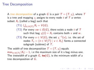
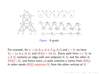
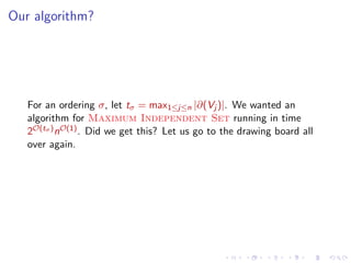
![We continue with Maximum Independent Set, now we try to
solve the problem for an arbitrary graph G . The idea is again to
perform dynamic programming, but this time instead of going from
leaves to the root, we go via separating set of vertices.
Let us fix an ordering σ = (v1 , v2 , . . . , vn ) of the vertices of G . For
j ∈ {1, 2, . . . , n}, we use Vj to denote the set of the first j vertices
of σ.
G [Vn ] = G . The boundary of Vj is the subset of vertices of Vj
adjacent to vertices outside Vj .](https://image.slidesharecdn.com/slidesintrototreewidth-140306100411-phpapp02/85/Introduction-to-Treewidth-12-320.jpg)


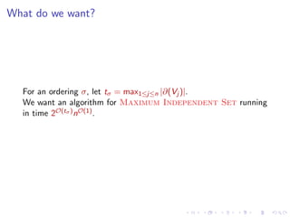


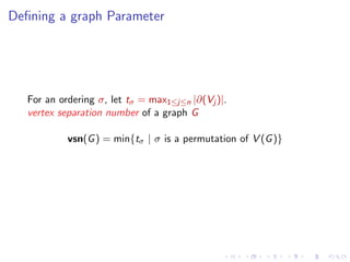
![Dynamic Table: Generalization of Party Argument
For every subset S of the boundary X , T [S] is the size of the
largest independent set I such that I ∩ X = S, or −∞ if no such
X
x1
x2
x3](https://image.slidesharecdn.com/slidesintrototreewidth-140306100411-phpapp02/85/Introduction-to-Treewidth-21-320.jpg)
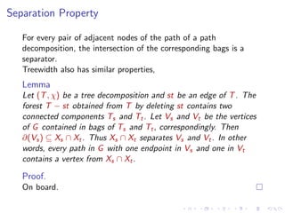
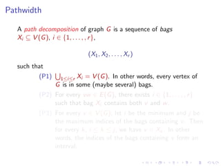
![Dynamic Table
The size of the largest independent set I such that I ∩ X = S, or
−∞ if no such set exists.
X
x1
x2
x3
T [∅]
T [x1 ]
T [x2 ]
T [x3 ]
T [x1 , x2 ]
T [x1 , x3 ]
T [x2 , x3 ]
T [x1 , x2 , x3 ]
4
4
3
3
−∞
3
3
−∞](https://image.slidesharecdn.com/slidesintrototreewidth-140306100411-phpapp02/85/Introduction-to-Treewidth-22-320.jpg)
![Dynamic Table
The size of the largest independent set I such that I ∩ X = S, or
−∞ if no such set exists.
X
x1
x2
x3
T [∅]
T [x1 ]
T [x2 ]
T [x3 ]
T [x1 , x2 ]
T [x1 , x3 ]
T [x2 , x3 ]
T [x1 , x2 , x3 ]
4
4
3
3
−∞
3
3
−∞](https://image.slidesharecdn.com/slidesintrototreewidth-140306100411-phpapp02/85/Introduction-to-Treewidth-23-320.jpg)
![Dynamic Table
The size of the largest independent set I such that I ∩ X = S, or
−∞ if no such set exists.
X
x1
x2
x3
T [∅]
T [x1 ]
T [x2 ]
T [x3 ]
T [x1 , x2 ]
T [x1 , x3 ]
T [x2 , x3 ]
T [x1 , x2 , x3 ]
4
4
3
3
−∞
3
3
−∞](https://image.slidesharecdn.com/slidesintrototreewidth-140306100411-phpapp02/85/Introduction-to-Treewidth-24-320.jpg)
![Dynamic Table
The size of the largest independent set I such that I ∩ X = S, or
−∞ if no such set exists.
X
x1
x2
x3
T [∅]
T [x1 ]
T [x2 ]
T [x3 ]
T [x1 , x2 ]
T [x1 , x3 ]
T [x2 , x3 ]
T [x1 , x2 , x3 ]
4
4
3
3
−∞
3
3
−∞](https://image.slidesharecdn.com/slidesintrototreewidth-140306100411-phpapp02/85/Introduction-to-Treewidth-25-320.jpg)
![Dynamic Table
The size of the largest independent set I such that I ∩ X = S, or
−∞ if no such set exists.
X
x1
x2
x3
T [∅]
T [x1 ]
T [x2 ]
T [x3 ]
T [x1 , x2 ]
T [x1 , x3 ]
T [x2 , x3 ]
T [x1 , x2 , x3 ]
4
4
3
3
−∞
3
3
−∞](https://image.slidesharecdn.com/slidesintrototreewidth-140306100411-phpapp02/85/Introduction-to-Treewidth-26-320.jpg)
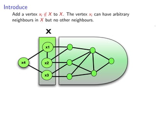
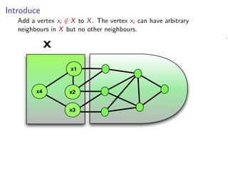
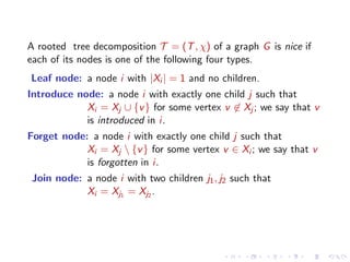
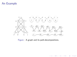
![Introduce: Updating the Table T
Suppose xi (here x4 ) was introduced into X , with closed
neighbourhood N[xi ]. We update the table T .
T [S]
if xi ∈ S,
/
T [S] = −∞
if xi ∈ S and S ∩ N(xi ) = ∅,
1 + T [S xi ] if xi ∈ S and S ∩ N(xi ) = ∅.
Update time: O(2t )](https://image.slidesharecdn.com/slidesintrototreewidth-140306100411-phpapp02/85/Introduction-to-Treewidth-29-320.jpg)
![Introduce: Updating the Table T
Suppose xi (here x4 ) was introduced into X , with closed
neighbourhood N[xi ]. We update the table T .
T [S]
if xi ∈ S,
/
T [S] = −∞
if xi ∈ S and S ∩ N(xi ) = ∅,
1 + T [S xi ] if xi ∈ S and S ∩ N(xi ) = ∅.
Update time: O(2t )](https://image.slidesharecdn.com/slidesintrototreewidth-140306100411-phpapp02/85/Introduction-to-Treewidth-30-320.jpg)
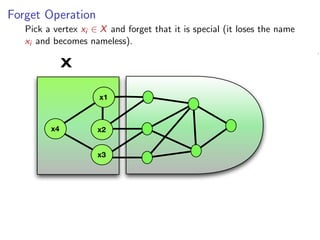

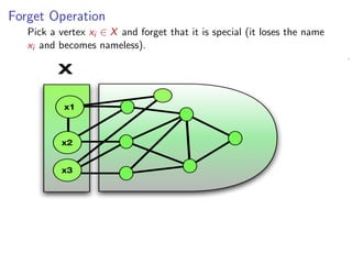
![Forget: Updating the Table T
Forgetting xi (here x4 ).
T [S] = max T [S], T [S ∪ xi ]
Update time: O(2t )](https://image.slidesharecdn.com/slidesintrototreewidth-140306100411-phpapp02/85/Introduction-to-Treewidth-34-320.jpg)


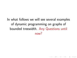
![Joining G1 and G2 : Updating the Table T for Maximum
Independent Set
Have a table T1 for G1 and T2 for G2 , want to compute the table
T for their join.
T [S] = T1[S] + T2[S] − |S|
Update time: O(2t )](https://image.slidesharecdn.com/slidesintrototreewidth-140306100411-phpapp02/85/Introduction-to-Treewidth-63-320.jpg)