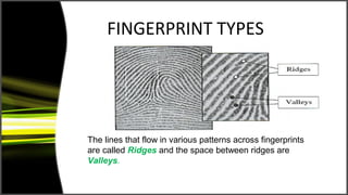
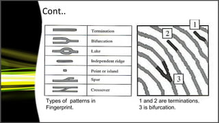
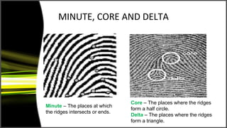
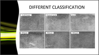
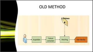
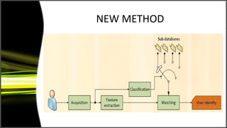
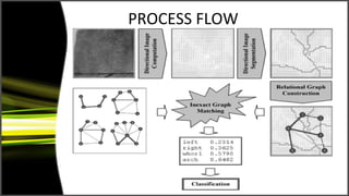
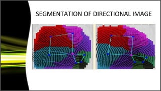
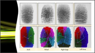
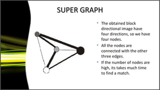
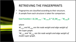
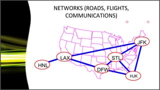
Graph theory has many applications including social networks, data organization, and communication networks. The document discusses Dijkstra's algorithm for finding the shortest path between nodes in a graph and its application to finding shortest routes between cities. It also discusses using graph representations for fingerprint classification, where fingerprints are modeled as graphs with nodes for fingerprint regions and edges between adjacent regions. Fingerprints are classified based on the structure of these graphs and compared to model graphs for matching.

1. APPLICATIONS OF GRAPHS

2. GRAPHS
• Graph theory has turned out to be a vast area with
innumerable applications in the field of social
networks , data organization , communication
network and so on…
• We have considered here
1.Dijkstra’s algorithm
2. Fingerprint classification using graph theory

3. DIJKSTRA’S
ALGORITHM

4. DIJKSTRA’S ALGORITHM
• Djikstra's algorithm (named after its discover, E.W.
Dijkstra) solves the problem of finding the shortest path
from a point in a graph (the source) to a destination.
• It turns out that one can find the shortest paths from a
given source to all points in a graph in the same time,
hence this problem is sometimes called the single-
source shortest paths problem.

5. • Given a network of cities and the distances between
them, the objective of the single-source, shortest-
path problem is to find the shortest path from a city
to all other cities connected to it.
• The network of cities with their distances is
represented as a weighted graph.

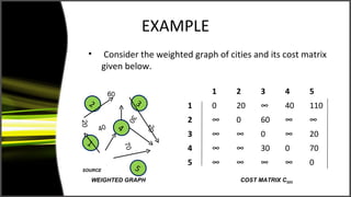
6. • Let V be a set of N cities (vertices) of the digraph. Here
the source city is 1.
• The set T is initialized to city 1.
• The DISTANCE vector, DISTANCE [2:N] initially records
the distances of cities 2 to N connected to the source
by an edge (not path!)
60
2 3
30
20 40 4
20
1
70
110
SOURCE 5

7. • If there is no edge directly connecting the city to
source, then we initialize its DISTANCE value to ‘∞’
• Once the algorithm completes iterations, the
DISTANCE vector holds the shortest distance of two
cities 2 to N from the source city 1
• It is convenient to represent the weighted digraph
using its cost matrix COSTN x N
• The cost matrix records the distances between cities
connected by an edge.
• Dijkstra’s algorithm has a complexity of O(N 2) where N
is the number of vertices (cities) in the weighted
digraph

8. DIJKSTRA’S ALGORITHM
Procedure DIJKSTRA_SSSP(N, COST)
/* N is the number of vertices labeled {1,2,3,….,N} of the weighted digraph. If
there is no edge then COST [I, j] = ∞ */
/* The procedure computes the cost of the shortest path from vertex 1 the
source, to every other vertex of the weighted digraph */
T = {1}; /* initialize T to source vertex */
for i = 2 to N do
DISTANCE [i] = COST [1,i];
/* initialize DISTANCE vector to the cost of the edges connecting vertex I with
the source vertex 1. If there is no edge then COST[1,i] = ∞ */

9. for i = 1 to N-1 do
Choose a vertex u in V – T such that DISTANCE [u] is a
minimum;
Add u to T;
for each vertex w in V – T do
DISTANCE [w] = minimum ( DISTANCE [w] , DISTANCE [u]
+ COST [u ,w]);
end
end
end DIJKSTRA_SSSP

10. EXAMPLE
• Consider the weighted graph of cities and its cost matrix
given below.
60 1 2 3 4 5
2 3 1 0 20 ∞ 40 110
2 ∞ 0 60 ∞ ∞
30
20
40 4
20
3 ∞ ∞ 0 ∞ 20
1
4 ∞ ∞ 30 0 70
70
5 ∞ ∞ ∞ ∞ 0
SOURCE
5
WEIGHTED GRAPH COST MATRIX C5X5

11. Trace of The Table following that shows the trace of the
Dijkstra’s algorithm

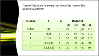
12. • The DISTANCE vector in the last iteration records the
shortest distance of the vertices {2,3,4,5} from the source
vertex 1.
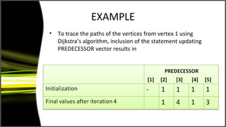
• To reconstruct the shortest path from the source vertex to
all other vertices, a vector PREDECESSOR [1:N] where
PREDECESSOR [v] records the predecessor of vertex v in the
shortest path, is maintained.
• PREDECESSOR [1:N] is initialized to source for all v != source

13. • PREDECESSOR [1:N] is updated by
if (( DISTANCE [u] + COST [u, w]) < DISTANCE [w])
then PREDECESSOR [w] = u
soon after DISTANCE [w] = minimum ( DISTANCE [w] ,
DISTANCE [u] + COST [u ,w]) is computed in procedure
DIJKSTRA_SSS
• To trace the shortest path we move backwards from the
destination vertex, hopping on the predecessors recorded by
the PREDECESSOR vector until the source vertex is reached

14. EXAMPLE
• To trace the paths of the vertices from vertex 1 using
Dijkstra’s algorithm, inclusion of the statement updating
PREDECESSOR vector results in

15. • To trace the shortest path from source 1 to vertex 5, we move
in the reverse direction from vertex 5 hopping on the
predecessors until the source vertex is reached. The shortest
path is given by
PREDECESSOR(5)=3 PREDECESSOR(3)=4 PREDECESSOR(4)=1
Vertex 5 Vertex 3 Vertex 4 Source Vertex 1
Thus the shortest path between vertex 1 and vertex 5 is
1-4-3-5 and the distance is given by DISTANCE [5] is 90

16. FINGERPRINT
RECOGNITION
USING GRAPH
REPRESENTATIO
N

17. The three characteristics of FINGER PRINTS are:
1. There are no similar fingerprints in the world.
2. Fingerprints are unchangeable.
3. Fingerprints are one of the unique features for
identification systems.

18. FINGERPRINT TYPES
The lines that flow in various patterns across fingerprints
are called Ridges and the space between ridges are
Valleys.

19. Cont..
Types of patterns in 1 and 2 are terminations.
Fingerprint. 3 is bifurcation.

20. MINUTE, CORE AND DELTA
Core – The places where the ridges
Minute – The places at which
form a half circle.
the ridges intersects or ends.
Delta – The places where the ridges
form a triangle.

21. DIFFERENT CLASSIFICATION

22. OLD METHOD

23. NEW METHOD

24. PROCESS FLOW

25. FINGERPRINT CAPTURE DEVICES

26. SEGMENTATION OF DIRECTIONAL IMAGE

28. SEGMENTATION

29. CONSTRUCTION OF RELATED WEIGHT
GRAPH
Graph can be shown by G index including four
parameters of G= (V, E, μ,υ).
where
V is number of nodes.
E is number of edges.
μ is weight of nodes.
υ is weight of edges.

30. Some information can be used in constructing the graph
related to a finger print like:
• Centre of gravity of regions.
• The direction related to the elements of the various
regions.
• The area of all the regions.
• The distance between centres of gravity.
• The perimeter of regions.

31. WEIGHTAGE TO NODES AND EDGES
Wn = Area (Ri)
where
 i = 1,2,3,……,n.
 Wn is the weight of nodes .
 Ri is the specified region in block directional image.
We = (Adj − p) × (Node − d) × (Diff −v)
where
 Adj-p is the boundary of two adjacent regions linking with an edge.
 Node-d is the distance difference between nodes that links by an edge
 Diff-v is the phase difference or direction difference between two
regions of block directional image.

32. The nodes are placed in the centre of gravity of
each region. The nodes size vary according to the
weight. The edges are shown by the lines and the
thickness is proportional to the weight .

33. CONSTRUCTING SUPER GRAPH
We combine the properties of the Graph and model of the
Super Graph to form,
• A node for region with similar directions.
• Its co-ordinates is the centre of gravity related to those
regions of the graph.

34. WEIGHTAGE TO sNODES AND sEDGES
Wsn = nΣi=1 Area (Ri)
Where
Area (Ri) is the area of all regions with similar directions.
Ri includes regions with similar directions.
Wse = dis(sn) + Σ Adj-p(Ri,Rj)
Where
Wse is the weight of edges in super graph.
dis(sn) is the distance between nodes of a super graph.
Adj-p is the sum of the adjacent perimeter between two
regions.

35. SUPER GRAPH
 The obtained block
directional image have
four directions, so we have
four nodes.
 All the nodes are
connected with the other
three edges.
 If the number of nodes are
high, its takes much time
to find a match.

36. RETRIEVING THE FINGERPRINTS
• Fingerprints are classified according to their structure.
• A sample from each structure is taken for comparison.
Cost Function = (Σi (Wi.node – *Wi.node )) * (Σj (Wj.edge - *Wj.edge))
where
Wi.node and Wj.edge are the node weight and edge weight of
the Super graph.
*
Wi.node and *Wj.edge are the node weight and edge weight of
model super graph.

37. • Different classifications give different cost value.Among
that the lowest cost value function is taken and the
comparison of the fingerprint proceeds in that class.
• By this method high accuracy is achieved in short
comparison time.
• Previously FBI used 3 major classifications for matching the
fingerprints and they had many sub-classifications.
• But now they use around 10 major classifications and
many sub-classifications which gives them a fast result.

38. SOME MORE INTERESTING
APPLICATIONS…..

39. EPIDEMOLOGY
• Networks model used to represent the
spread of infectious diseases and design
prevention and response strategies.
• Vertices represent individuals, and edges
their possible contacts. It is useful to
calculate how a particular individual is
connected to others.
• Knowing the shortest path lengths to
other individuals can be a relevant
indicator of the potential of a particular
individual to infect others.

40. SOCIAL NETWORKS

41. NETWORKS (ROADS, FLIGHTS,
COMMUNICATIONS)
JFK
LAX STL
HNL
DFW
HJK

42. THANK YOU!!!