This document discusses the synthesis and optimization of digital signal processing (DSP) algorithms, emphasizing the growth and importance of DSP in various fields, such as speech recognition and biomedical instrumentation. It explores techniques for automating the creation of area-efficient designs from high-level descriptions of DSP algorithms, particularly in light of increasing computational demands. The book serves as a resource for those at the intersection of DSP algorithm design and implementation, detailing methods applicable to both linear and nonlinear systems.


![1
Introduction
1.1 Objectives
This book addresses the problem of hardware synthesis from an initial, in-
finite precision, specification of a digital signal processing (DSP) algorithm.
DSP algorithm development is often initially performed without regard to fi-
nite precision effects, whereas in digital systems values must be represented to
a finite precision [Mit98]. Finite precision representations can lead to undesir-
able effects such as overflow errors and quantization errors (due to roundoff or
truncation). This book describes methods to automate the translation from an
infinite precision specification, together with bounds on acceptable errors, to
a structural description which may be directly implemented in hardware. By
automating this step, raise the level of abstraction at which a DSP algorithm
can be specified for hardware synthesis.
We shall argue that, often, the most efficient hardware implementation of
an algorithm is one in which a wide variety of finite precision representations
of different sizes are used for different internal variables. The size of the rep-
resentation of a finite precision ‘word’ is referred to as its word-length. Imple-
mentations utilizing several different word-lengths are referred to as ‘multiple
word-length’ implementations and are discussed in detail in this book.
The accuracy observable at the outputs of a DSP system is a function of
the word-lengths used to represent all intermediate variables in the algorithm.
However, accuracy is less sensitive to some variables than to others, as is
implementation area. It is demonstrated in this book that by considering error
and area information in a structured way using analytical and semi-analytical
noise models, it is possible to achieve highly efficient DSP implementations.
Multiple word-length implementations have recently become a flourishing
area of research [KWCM98, WP98, CRS+
99, SBA00, BP00, KS01, NHCB01].
Stephenson [Ste00] enumerates three target areas for this research: SIMD
architectures for multimedia [PW96], power conservation in embedded sys-
tems [BM99], and direct hardware implementations. Of these areas, this book](https://image.slidesharecdn.com/optimizationandpreparationprocesses-240125021124-f0b0fb42/85/optimization-and-preparation-processes-pdf-14-320.jpg)
![2 1 Introduction
targets the latter, although Chapters 3 to 5 could form the basis of an ap-
proach to the first two application areas.
Throughout the book, both the word-length of operations, and the overflow
methods used, are considered to be optimization variables for minimizing the
area or power consumption of a hardware implementation. At the same time,
they impost constraints on possible solutions on the basis of signal quality
at the system outputs. The resulting multiple word-length implementations
pose new challenges to the area of high-level synthesis [Cam90], which are also
addressed in this book.
1.2 Overview
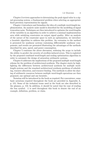
The overall design flow proposed and discussed is illustrated in Fig. 1.1. Each
of the blocks in this diagram will be discussed in more detail in the chapters
to follow.
multiple
word-length
libraries
Simulink signal
scaling
wordlength
optimization
combined
scaling
and
wordlength
optimization
bit-true
simulator
resource
sharing
(Chapter 6)
synthesis of
structural HDL
error
constraints
(Chapter 3) (Chapter 5)
vendor
synthesis
completed
design
HDL
libraries
(Chapter 4) library
cost models
Fig. 1.1. System design flow and relationship between chapters
We begin in Chapter 2 by reviewing some relevant backgroud material,
including a very brief introduction to important nomenclature in DSP, digital
design, and algorithm representation. The key idea here is that in an efficient
hardware implementation of a DSP algorithm, the representation used for each
signal can be different from that used for other signals. Our representation
consists of two parts: the scaling and the word-length. The optimization of
these two parts are covered respectively in Chapters 3 and 4.](https://image.slidesharecdn.com/optimizationandpreparationprocesses-240125021124-f0b0fb42/85/optimization-and-preparation-processes-pdf-15-320.jpg)

![2
Background
This chapter provides some of the necessary background required for the rest
of this book. In particular, since this book is likely to be of interest both
to DSP engineers and digital designers, a basic introduction to the essential
nomenclature within each of these fields is provided, with references to further
material as required.
Section 2.1 introduces microprocessors and field-programmable gate ar-
rays. Section 2.2 then covers the discrete-time description of signals using
the z-transform. Finally, Section 2.3 presents the representation of DSP al-
gorithms using computation graphs.
2.1 Digital Design for DSP Engineers
2.1.1 Microprocessors vs. Digital Design
One of the first options faced by the designer of a digital signal processing
system is whether that system should be implemented in hardware or soft-
ware. A software implementation forms an attractive possibility, due to the
mature state of compiler technology, and the number of good software en-
gineers available. In addition microprocessors are mass-produced devices and
therefore tend to be reasonably inexpensive. A major drawback of a micro-
processor implementation of DSP algorithms is the computational throughput
achievable. Many DSP algorithms are highly parallelizable, and could benefit
significantly from more fine-grain parallelism than that available with gen-
eral purpose microprocessors. In response to this acknowledged drawback,
general purpose microprocessor manufacturers have introduced extra single-
instruction multiple-data (SIMD) instructions targetting DSP such as the
Intel MMX instruction set [PW96] and Sun’s VIS instruction set [TONH96].
In addition, there are microprocessors specialized entirely for DSP such as the
well-known Texas Instruments DSPs [TI]. Both of these implementations al-
low higher throughput than that achievable with a general purpose processor,
but there is still a significant limit to the throughput achievable.](https://image.slidesharecdn.com/optimizationandpreparationprocesses-240125021124-f0b0fb42/85/optimization-and-preparation-processes-pdf-18-320.jpg)
![6 2 Background
The alternative to a microprocessor implementation is to implement the
algorithm in custom digital hardware. This approach brings dividends in the
form of speed and power consumption, but suffers from a lack of mature
high-level design tools. In digital design, the industrial state of the art is
register-transfer level (RTL) synthesis [IEE99, DC]. This form of design in-
volves explicitly specifying the cycle-by-cycle timing of the circuit and the
word-length of each signal within the circuit. The architecture must then be
encoded using a mixture of data path and finite state machine constructs. The
approaches outlined in this book allow the production of RTL-synthesizable
code directly from a specification format more suitable to the DSP application
domain.
2.1.2 The Field-Programmable Gate Array
There are two main drawbacks to designing an application-specific integrated
circuit (ASICs) for a DSP application: money and time. The production of
state of the art ASICs is now a very expensive process, which can only real-
istically be entertained if the market for the device can be counted in millions
of units. In addition, ASICs need a very time consuming test process before
manufacture, as ‘bug fixes’ cannot be created easily, if at all.
The Field-Programmable Gate Array (FPGA) can overcome both these
problems. The FPGA is a programmable hardware device. It is mass-produced,
and therefore can be bought reasonably inexpensively, and its programmabil-
ity allows testing in-situ. The FPGA can trace its roots from programmable
logic devices (PLDs) such as PLAs and PALs, which have been readily avail-
able since the 1980s. Originally, such devices were used to replace discrete
logic series in order to minimize the number of discrete devices used on a
printed circuit board. However the density of today’s FPGAs allows a single
chip to replace several million gates [Xil03]. Under these circumstances, using
FPGAs rather than ASICs for computation has become a reality.
There are a range of modern FPGA architectures on offer, consisting of
several basic elements. All such architectures contain the 4-input lookup table
(4LUT or simply LUT) as the basic logic element. By configuring the data
held in each of these small LUTs, and by configuring the way in which they
are connected, a general circuit can be implemented. More recently, there
has been a move towards heterogeneous architectures: modern FPGA devices
such as Xilinx Virtex also contain embedded RAM blocks within the array
of LUTs, Virtex II adds discrete multiplier blocks, and Virtex II pro [Xil03]
adds PowerPC processor cores.
Although many of the approaches described in this book can be applied
equally to ASIC and FPGA-based designs, it is our belief that programmable
logic design will continue to increase its share of the market in DSP applic-
ations. For this reason, throughout this book, we have reported results from
these methods when applied to FPGAs based on 4LUTs.](https://image.slidesharecdn.com/optimizationandpreparationprocesses-240125021124-f0b0fb42/85/optimization-and-preparation-processes-pdf-19-320.jpg)
![2.1 Digital Design for DSP Engineers 7
2.1.3 Arithmetic on FPGAs
Two arithmetic operations together dominate DSP algorithms: multiplication
and addition. For this reason, we shall take the opportunity to consider how
multiplication and addition are implemented in FPGA architectures. A basic
understanding of the architectural issues involved in designing adders and
multipliers is key to understanding the area models derived in later chapters
of this book.
Many hardware architectures have been proposed in the past for fast ad-
dition. As well as the simple ripple-carry approach, these include carry-look-
ahead, conditional sum, carry-select, and carry-skip addition [Kor02]. While
the ASIC designer typically has a wide choice of adder implementations, most
modern FPGAs have been designed to support fast ripple-carry addition. This
means that often, ‘fast’ addition techniques are actually slower than ripple-
carry in practice. For this reason, we restrict ourselves to ripple carry addition.
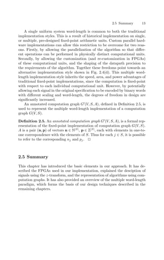
Fig. 2.1 shows a portion of the Virtex II ‘slice’ [Xil03], the basic logic unit
within the Virtex II FPGA. As well as containing two standard 4LUTs, the
slice contains dedicated multiplexers and XOR gates. By using the LUT to
generate the ‘carry propagate’ select signal of the multiplexer, a two-bit adder
can be implemented within a single slice.
4LUT 4LUT
carry
in
carry
out
adder inputs
adder outputs
Fig. 2.1. A Virtex II slice configured as a 2-bit adder](https://image.slidesharecdn.com/optimizationandpreparationprocesses-240125021124-f0b0fb42/85/optimization-and-preparation-processes-pdf-20-320.jpg)
![8 2 Background
In hardware arithmetic design, it is usual to separate the two cases of
multiplier design: when one operand is a constant, and when both operands
may vary. In the former case, there are many opportunities for reducing the
hardware cost and increasing the hardware speed compared to the latter case.
A constant-coefficient multiplication can be re-coded as a sum of shifted ver-
sions of the input, and common sub-expression elimination techniques can be
applied to obtain an efficient implementation in terms of adders alone [Par99]
(since shifting is free in hardware). General multiplication can be performed
by adding partial products, and general multipliers essentially differ in the
ways they accumulate such partial products. The Xilinx Virtex II slice, as
well as containing a dedicated XOR gate for addition, also contains a dedic-
ated AND gate, which can be used to calculate the partial products, allowing
the 4LUTs in a slice to be used for their accumulation.
2.2 DSP for Digital Designers
A signal can be thought of as a variable that conveys information. Often
a signal is one dimensional, such as speech, or two dimensional, such as an
image. In modern communication and computation, such signals are often
stored digitally. It is a common requirement to process such a signal in order
to highlight or supress something of interest within it. For example, we may
wish to remove noise from a speech signal, or we may wish to simply estimate
the spectrum of that signal.
By convention, the value of a discrete-time signal x can be represented by a
sequence x[n]. The index n corresponds to a multiple of the sampling period T ,
thus x[n] represents the value of the signal at time nT . The z transform (2.1)
is a widely used tool in the analysis and processing of such signals.
X(z) =
+∞
n=−∞
x[n]z−n
(2.1)
The z transform is a linear transform, since if X1(z) is the transform of
x1[n] and X2(z) is the transform of x2[n], then αX1(z) + βX2(z) is the trans-
form of αx1[n] + βx2[n] for any real α, β. Perhaps the most useful property of
the z transform for our purposes is its relationship to the convolution oper-
ation. The output y[n] of any linear time-invariant (LTI) system with input
x[n] is given by (2.2), for some sequence h[n].
y[n] =
+∞
k=−∞
h[k]x[n − k] (2.2)
Here h[n] is referred to as the impulse response of the LTI system, and is
a fixed property of the system itself. The z transformed equivalent of (2.2),
where X(z) is the z transform of the sequence x[n], Y (z) is the z transform](https://image.slidesharecdn.com/optimizationandpreparationprocesses-240125021124-f0b0fb42/85/optimization-and-preparation-processes-pdf-21-320.jpg)
![2.3 Computation Graphs 9
of the sequence y[n] and H(z) is the z transform of the sequence h[n], is given
by (2.3). In these circumstances, H(z) is referred to as the transfer function.
Y (z) = H(z)X(z) (2.3)
For the LTI systems discussed in this book, the system transfer function
H(z) takes the rational form shown in (2.4). Under these circumstances, the
values {z1, z2, . . . , zm} are referred to as the zeros of the transfer function and
the values {p1, p2, . . . , pn} are referred to as the poles of the transfer function.
H(z) = K
(z−1
− z−1
1 )(z−1
− z−1
2 ) . . . (z−1
− z−1
m )
(z−1 − p−1
1 )(z−1 − p−1
2 ) . . . (z−1 − p−1
n )
(2.4)
2.3 Computation Graphs
Synchronous Data Flow (SDF) is a widely used paradigm for the representa-
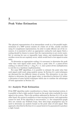
tion of digital signal processing systems [LM87b], and underpins several com-
merical tools such as Simulink from The MathWorks [SIM]. A simple example
diagram from Simulink is shown in Fig. 2.2. Such a diagram is intuitive as
a form of data-flow graph, a concept we shall formalize shortly. Each node
represents an operation, and conceptually a node is ready to execute, or ‘fire’,
if enough data are present on all its incoming edges.
Fig. 2.2. A simple Simulink block diagram
In some chapters, special mention will be made of linear time invariant
(LTI) systems. Individual computations in an LTI system can only be one of
several types: constant coefficient multiplication, unit-sample delay, addition,
or branch (fork). Of course the representation of an LTI system can be of a](https://image.slidesharecdn.com/optimizationandpreparationprocesses-240125021124-f0b0fb42/85/optimization-and-preparation-processes-pdf-22-320.jpg)
![10 2 Background
hierarchical nature, in terms of other LTI systems, but each leaf node of any
such representation must have one of these four types. A flattened LTI rep-
resentation forms the starting point for many of the optimization techniques
described.
We will discuss the representation of LTI systems, on the understanding
that for differentiable nonlinear systems, used in Chapter 4, the representation
is identical with the generalization that nodes can form any differentiable
function of their inputs.
The representation used is referred to as a computation graph (Defini-
tion 2.1). A computation graph is a specialization of the data-flow graphs of
Lee et al. [LM87b].
Definition 2.1. A computation graph G(V, S) is the formal representation of
an algorithm. V is a set of graph nodes, each representing an atomic computa-
tion or input/output port, and S ⊂ V ×V is a set of directed edges representing
the data flow. An element of S is referred to as a signal. The set S must satisfy
the constraints on indegree and outdegree given in Table 2.1 for LTI nodes.
The type of an atomic computation v ∈ V is given by type(v) (2.5). Further,
if VG denotes the subset of V with elements of gain type, then coef : VG → R
is a function mapping the gain node to its coefficient.
type : V → {inport, outport, add, gain, delay, fork} (2.5)
Table 2.1. Degrees of nodes in a computation graph
type(v) indegree(v) outdegree(v)
inport 0 1
outport 1 0
add 2 1
delay 1 1
gain 1 1
fork 1 ≥ 2
Often it will be useful to visualize a computation graph using a graphical
representation, as shown in Fig. 2.3. Adders, constant coefficient multipliers
and unit sample delays are represented using different shapes. The coefficient
of a gain node can be shown inside the triangle corresponding to that node.
Edges are represented by arrows indicating the direction of data flow. Fork
nodes are implicit in the branching of arrows. inport and outport nodes
are also implicitly represented, and usually labelled with the input and output
names, x[t] and y[t] respectively in this example.](https://image.slidesharecdn.com/optimizationandpreparationprocesses-240125021124-f0b0fb42/85/optimization-and-preparation-processes-pdf-23-320.jpg)
![2.3 Computation Graphs 11
x[t] y[t]
+
(b) an example computation graph
+
z
-1
z
-1
ADD GAIN DELAY FORK
(a) some nodes in a computation graph
COEF
Fig. 2.3. The graphical representation of a computation graph
Definition 2.1 is sufficiently general to allow any multiple input, multiple
output (MIMO) LTI system to be modelled. Such systems include operations
such as FIR and IIR filtering, Discrete Cosine Transforms (DCT) and RGB
to YCrCb conversion. For a computation to provide some useful work, its
result must be in some way influenced by primary external inputs to the sys-
tem. In addition, there is no reason to perform a computation whose result
cannot influence external outputs. These observations lead to the definition
of a well-connected computation graph (Definition 2.2). The computability
property (Definition 2.4) for systems containing loops (Definition 2.3) is also
introduced below. These definitions become useful when analyzing the proper-
ties of certain algorithms operating on computation graphs. For readers from
a computer science background, the definition of a recursive system (Defin-
ition 2.3) should be noted. This is the standard DSP definition of the term
which differs from the software engineering usage.
Definition 2.2. A computation graph G(V, S) is well-connected iff (a) there
exists at least one directed path from at least one node of type inport to
each node v ∈ V and (b) there exists at least one directed path from each
node in v ∈ V to at least one node of type outport.
Definition 2.3. A loop is a directed cycle (closed path) in a computation
graph G(V, S). The loop body is the set of all vertices V1 ⊂ V in the loop. A
computation graph containing at least one loop is said to describe a recursive
system.](https://image.slidesharecdn.com/optimizationandpreparationprocesses-240125021124-f0b0fb42/85/optimization-and-preparation-processes-pdf-24-320.jpg)
![12 2 Background
Definition 2.4. A computation graph G is computable iff there is at least one
node of type delay contained within the loop body of each loop in G.
2.4 The Multiple Word-Length Paradigm
Throughout this book, we will make use of a number representation known
as the multiple word-length paradigm [CCL01b]. The multiple word-length
paradigm can best be introduced by comparison to more traditional fixed-
point and floating-point implementations. DSP processors often use fixed-
point number representations, as this leads to area and power efficient imple-
mentations, often as well as higher throughput than the floating-point altern-
ative [IO96]. Each two’s complement signal j ∈ S in a multiple word-length
implementation of computation graph G(V, S), has two parameters nj and pj,
as illustrated in Fig. 2.4(a). The parameter nj represents the number of bits
in the representation of the signal (excluding the sign bit), and the parameter
pj represents the displacement of the binary point from the LSB side of the
sign bit towards the least-significant bit (LSB). Note that there are no restric-
tions on pj; the binary point could lie outside the number representation, i.e.
pj 0 or pj nj.
(c)
(n,v(t)) (n,w(t)) (n,x(t))
+
(n,z(t))
(d)
(n,0) (n,0) (n,0)
+
(n,0)
(b)
(a,v) (b,w) (c,x)
+
(d,y)
p
...
S
n
(a)
(n,0)
(e,z)
(n,y(t))
Fig. 2.4. The Multiple Word-Length Paradigm: (a) signal parameters (‘s’ indicates
sign bit), (b) fixed-point, (c) floating-point, (d) multiple word-length
A simple fixed-point implementation is illustrated in Fig. 2.4(b). Each
signal j in this block diagram representing a recursive DSP data-flow, is an-
notated with a tuple (nj, pj) showing the word-length nj and scaling pj of the
signal. In this implementation, all signals have the same word-length and scal-
ing, although shift operations are often incorporated in fixed-point designs,
in order to provide an element of scaling control [KKS98]. Fig. 2.4(c) shows a
standard floating-point implementation, where the scaling of each signal is a
function of time.](https://image.slidesharecdn.com/optimizationandpreparationprocesses-240125021124-f0b0fb42/85/optimization-and-preparation-processes-pdf-25-320.jpg)

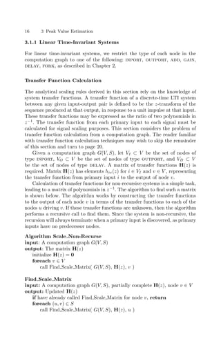
![18 3 Peak Value Estimation
A(z) = 0.1z−1
B(z) = 1
C(z) = [0 1 0.1 0.1 0.1 0.1z−1
]T
D(z) = [1 0 0 0 0 0]T
(3.4)
+
x[t] y[t]
z
-1
0 1a 2 3
4
5
1b
Fig. 3.1. An example of transfer function calculation (each signal has been labelled
with a signal number)
Calculation of S(z) proceeds following (3.3), yielding (3.5). Finally, the
matrix H(z) can be constructed following (3.2), giving (3.6).
S(z) =
1
1 − 0.1z−1
(3.5)
H(z) = [1
1
1 − 0.1z−1
0.1
1 − 0.1z−1
0.1
1 − 0.1z−1
0.1
1 − 0.1z−1
0.1z−1
1 − 0.1z−1
]T
(3.6)
It is possible that the matrix inversion (I − A)−1
for calculation of S
dominates the overall computational complexity, since the matrix inversion
requires |Vc|3
operations, each of which is a polynomial multiplication. The
maximum order of each polynomial is |VD|. This means that the number of
scalar multiplications required for the matrix inversion is bounded from above
by |Vc|3
|VD|2
. It is therefore important from a computational complexity (and
memory requirement) perspective to make Vc as small as possible.
If the computation graph G(V, S) is computable, it is clear that Vc = VD is
one possible set of state nodes, bounding the minimum size of Vc from above.
If G(V, S) is non-recursive, Vc = ∅ is sufficient. The general problem of finding
the smallest possible Vc is well known in graph theory as the ‘minimum feed-
back vertex set’ problem [SW75, LL88, LJ00]. While the problem is known to
be NP-hard for general graphs [Kar72], there are large classes of graphs for
which polynomial time algorithms are known [LJ00]. However, since transfer
function calculation does not require a minimum feedback vertex set, we sug-
gest the algorithm of Levy and Low [LL88] be used to obtain a small feedback](https://image.slidesharecdn.com/optimizationandpreparationprocesses-240125021124-f0b0fb42/85/optimization-and-preparation-processes-pdf-31-320.jpg)
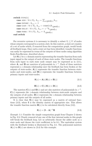
![3.1 Analytic Peak Estimation 21
to choose the smallest possible value of pj for each signal j ∈ S in order to
guarantee no overflow.
Consider an annotated computation graph G
(V, S, A), with A = (n, p).
Let VI ⊂ V be the set of inports, each of which reaches peak signal val-
ues of ±Mi (Mi 0) for i ∈ VI. Let H(z) be the scaling transfer func-
tion matrix defined in Section 3.1.1, with associated impulse response matrix
h[t] = Z−1
{H(z)}. Then the worst-case peak value Pj reached by any signal
j ∈ S is given by maximizing the well known convolution sum (3.7) [Mit98],
where xi[t] is the value of the input i ∈ VI at time index t. Solving this max-
imization problem provides the input sequence given in (3.8), and allowing
Nij → ∞ leads to the peak response at signal j given in (3.9). Here sgn(·) is
the signum function (3.10).
Pj = ±
i∈VI
max
xi[t]
Nij−1
t=0
xi[t
− t]hij[t]
(3.7)
xi[t] = Mi sgn(hij[Nij − t − 1]) (3.8)
Pj =
i∈VI
Mi
∞
t=0
|hij[t]| (3.9)
sgn(x) =
1, x ≥ 0
−1, otherwise
(3.10)
This worst-case approach leads to the concept of 1 scaling, defined in
Definitions 3.2 and 3.3.
Definition 3.2. The 1-norm of a transfer function H(z) is given by (3.11),
where Z−1
{·} denotes the inverse z-transform.
1{H(z)} =
∞
t=0
|Z−1
{H(z)}[t]| (3.11)
Definition 3.3. The annotated computation graph G
(V, S, A) is said to be
1-scaled iff (3.12) holds for all signals j ∈ S. Here VI, Mi and hij(z) are as
defined in the preceding paragraphs.
pj =
log2
i∈VI
Mi1{hij(z)} + 1 (3.12)](https://image.slidesharecdn.com/optimizationandpreparationprocesses-240125021124-f0b0fb42/85/optimization-and-preparation-processes-pdf-34-320.jpg)
![22 3 Peak Value Estimation
3.1.2 Data-range Propagation
If the algorithm under consideration is not linear, or is not time-invariant,
then one mechanism for estimating the peak value reached by each signal is
to consider the propagation of data ranges through the computation graph.
This is only possible for non-recursive algorithms.
Forward Propagation
A naïve way of approaching this problem is to examine the binary point
position “naturally” resulting from each hardware operator. Such an approach,
illustrated below, is an option in the Xilinx system generator tool [HMSS01].
Consider the computation graph shown in Fig. 3.3. If we consider that
each input has a range (−1, 1), then we require a binary point location of
p = log2 max |(−1, 1)| + 1 = 0 at each input. Let us consider each of the
adders in turn. Adder a1 adds two inputs with p = 0, and therefore produces
an output with p = max(0, 0)+1 = 1. Adder a2 adds one input with p = 0 and
one with p = 1, and therefore produces an output with p = max(0, 1)+1 = 2.
Similarly, the output of a3 has p = 3, and the output of a4 has p = 4. While we
have successfully determined a binary point location for each signal that will
not lead to overflow, the disadvantage of this approach should be clear. The
range of values reachable by the system output is actually 5∗(−1, 1) = (−5, 5),
so p = log2 max(−5, 5) + 1 = 3 is sufficient; p = 4 is an overkill of one MSB.
+ + + +
a1 a2 a3 a4
Fig. 3.3. A computation graph representing a string of additions
A solution to this problem that has been used in practice, is to propagate
data ranges rather than binary point locations [WP98, BP00]. This approach
can be formally stated in terms of interval analysis. Following [BP00],
Definition 3.4. An interval extension, denoted by f(x1, x2, . . . xn), of a real
function f(x1, x2, . . . , xn) is defined as any function of the n intervals x1, x2,
. . . , xn that evaluates to the value of f when its arguments are the degenerate
intervals x1, x2, . . . , xn, i.e.
f(x1, x2, . . . , xn) = f(x1, x2, . . . , xn) (3.13)](https://image.slidesharecdn.com/optimizationandpreparationprocesses-240125021124-f0b0fb42/85/optimization-and-preparation-processes-pdf-35-320.jpg)
![3.1 Analytic Peak Estimation 23
Definition 3.5. If xi ⊆ yi, for i = 1, 2, . . . , n and f(x1, x2, . . . , xn) ⊂
f(y1, y2, . . . , yn), then the interval extension f(X) is said to be inclusion
monotonic.
Let us denote by fr
(x1, x2, . . . , xn) the range of function f over the given
intervals. We may then use the result that fr
(x1, x2, . . . , xn) ⊆ f(x1, x2, . . . , xn)
[Moo66] to find an upper-bound on the range of the function.
Let us apply this technique to the example of Fig. 3.3. We may think of
each node in the computation graph as implementing a distinct function. For
addition, f(x, y) = x + y, and we may define the inclusion monotonic interval
extension f((x1
, x2
), (y1
, y2
)) = (x1
+ y1
, x2
+ y2
). Then the output of adder
a1 is a subset of (−2, 2) and thus is assigned p = 1, the output of adder a2
is a subset of (−3, 3) and is thus assigned p = 2, the output of adder a3 is a
subset of (−4, 4) and is thus assigned p = 3, and the output of adder a4 is
a subset of (−5, 5) and is thus assigned p = 3. For this simple example, the
problem of peak-value detection has been solved, and indeed fr
= f.
However, such a tight solution is not always possible with data-range
propagation. Under circumstances where the DFG contains one or more
branches (fork nodes), which later reconverge, such a “local” approach to
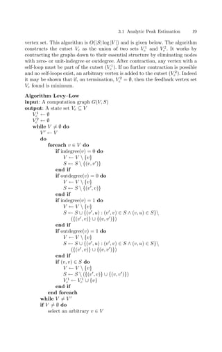
range propagation can be overly pessimistic. As an example, consider the
computation graph representing a complex constant coefficient multiplication
shown in Fig. 3.4.
(−0.6,0.6)
−1.6
(−0.96,0.96)
(−0.6,0.6)
+
(−3.12,3.12)
x [n]
2
x [n]
1
y [n]
1
y [n]
2
(−0.6,0.6)
2.1
+
(−0.6,0.6)
(−0.6,0.6)
(−0.6,0.6)
(−1.2,1.2)
−1.8
+
(−1.26,1.26)
(−2.16,2.16)
(−2.16,2.16)
(−3.42,3.42)
(−2.16,2.16)
−1
(−2.16,2.16)
Fig. 3.4. Range propagation through a computation graph
Each signal has been labelled with a propagated range, assuming that the
primary inputs have range (−0.6, 0.6). Under this approach, both outputs](https://image.slidesharecdn.com/optimizationandpreparationprocesses-240125021124-f0b0fb42/85/optimization-and-preparation-processes-pdf-36-320.jpg)
![24 3 Peak Value Estimation
require p = 2. However such ranges are overly pessimistic. The upper output
in Fig. 3.4 is clearly seen to have the value y1 = 2.1x1 −1.8(x1 +x2) = 0.3x1 −
1.8x2. Thus the range of this output can also be calculated as 0.3(−0.6, 0.6)−
1.8(−0.6, 0.6) = (−1.26, 1.26). Similarly for the lower output y2 = −1.6x2 +
1.8(x1+x2) = 1.8x1+0.2x2, providing a range 1.8(−0.6, 0.6)+0.2(−0.6, 0.6) =
(−1.2, 1.2). Thus by examining the global system behaviour, we can see that
in reality p = 1 is sufficient for both outputs. Note that the analytic scheme
described in Section 3.1.1 would calculate the tighter bound in this case.
In summary, range-propagation techniques may provide larger bounds on
signal values than those absolutely necessary. This problem is seen in extremis
with any recursive computation graph. In these cases, it is impossible to use
range-propagation to place a finite bound on signal values, even in cases when
such a finite bound can analytically be shown to exist.
3.2 Simulation-based Peak Estimation
A completely different approach to peak estimation is to use simulation: actu-
ally run the algorithm with a provided input data set, and measure the peak
value reached by each signal.
In its simplest form, the simulation approach consists of measuring the
peak signal value Pj reached by a signal j ∈ S and then setting p =
log2 kPj + 1, where k 1 is a user-supplied ‘safety factor’ typically having
value 2 to 4. Thus it is ensured that no overflow will occur, so long as the
signal value doesn’t exceed P̂j = kPj when excited by a different input se-
quence. Particular care must therefore be taken to select an appropriate test
sequence.
Kim and Kum [KKS98] extend the simulation approach by considering
more complex forms of ‘safety factor’. In particular, it is possible to try to
extract information from the simulation relating to the class of probability
density function followed by each signal. A histogram of the data values for
each signal is built, and from this histogram the distribution is classified as:
unimodal or multimodal, symmetric or non-symmetric, zero mean or non-zero
mean.
For a unimodal symmetric distribution, Kim and Kum propose the heur-
istic safety scaling P̂j = |µj| + (κj + 4)σj, where µj is the sample mean, κj
is the sample kurtosis, and σj is the sample standard deviation (all measured
during simulation).
For multimodal or non-symmetric distrubtion, the heuristic safety scaling
P̂j = P99.9%
j + 2(P100%
j − P99.9%
j ), has been proposed where Pp%
j represents
the simulation-measured p’th percentile of the sample.
In order to partially alleviate the dependence of the resulting scaling on the
particular input data sequence chosen, it is possible to simulate with several
different data sets. Let the maximum and minimum values of the standard
deviation (over the different data sets) be denoted σmax and σmin respectively.](https://image.slidesharecdn.com/optimizationandpreparationprocesses-240125021124-f0b0fb42/85/optimization-and-preparation-processes-pdf-37-320.jpg)
![3.4 Summary 25
Then the proposal of Kim and Kum [KKS98] is to use the heuristic estimate
σ = 1.1σmax − 0.1σmin. A similar approach is proposed for the other collected
statistics.
Simulation approaches are appropriate for nonlinear or time-varying sys-
tems, for which the data-range propagation approach described in Section 3.1.2
provides overly pessimistic results (such as for recursive systems). The main
drawback of simulation-based approaches is the significant dependence on the
input data set used for simulation; moreover no general guidelines can be
given for how to select an appropriate input.
3.3 Hybrid Techniques
Simulation can be combined with data-range propagation in order to try and
combine the advantages of the two techniques [CRS+
99, CH02].
A pure simulation, without ‘safety factor’, may easily underestimate the
required data range of a signal. Thus the scaling resulting from a simulation
can be considered as a lower-bound. In contrast, a pure data-range propaga-
tion will often significantly overestimate the required range, and can thus
be considered as an upper-bound. Clearly if the two approaches result in an
identical scaling assignment for a signal, the system can be confident that
simulation has resulted in an optimum scaling assignment. The question of
what the system should do with signals where the two scalings do not agree
is more complex.
Cmar et al. [CRS+
99] propose the heuristic distinction between those sim-
ulation and propagation scalings which are ‘significantly different’ and those
which are not. In the case that the two scalings are similar, say different by
one bit position, it may not be a significant hardware overhead to simply use
the upper-bound derived from range propagation.
If the scalings are significantly different, one possibility is to use satura-
tion arithmetic logic to implement the node producing the signal. When an
overflow occurs in saturation arithmetic, the logic saturates the output value
to the maximum positive or negative value representable, rather than causing
a two’s complement wrap-around effect. In effect the system acknowledges it
‘does not know’ whether the signal is likely to overflow, and introduces extra
logic to try and mitigate the effects of any such overflow. Saturation arithmetic
will be considered in much more detail in Chapter 5.
3.4 Summary
This chapter has covered several methods for estimating the peak value that
a signal can reach, in order to determine an appropriate scaling for that sig-
nal, resulting in an efficient representation. We have examined both analytic](https://image.slidesharecdn.com/optimizationandpreparationprocesses-240125021124-f0b0fb42/85/optimization-and-preparation-processes-pdf-38-320.jpg)

![4
Word-Length Optimization
The previous chapter described different techniques to find a scaling, or binary
point location, for each signal in a computation graph. This chapter addresses
the remaining signal parameter: its word-length.
The major problem in word-length optimization is to determine the error
at system outputs for a given set of word-lengths and scalings of all internal
variables. We shall call this problem error estimation. Once a technique for
error estimation has been selected, the word-length selection problem reduces
to utilizing the known area and error models within a constrained optimization
setting: find the minimum area implementation satisfying certain constraints
on arithmetic error at each system output.
The majority of this chapter is therefore taken up with the problem of error
estimation (Section 4.1). After discussion of error estimation, the problem
of area modelling is addressed in Section 4.2, after which the word-length
optimization problem is formulated and analyzed in Section 4.3. Optimization
techniques are introduced in Section 4.4 and Section 4.5, results are presented
in Section 4.6 and conclusions are drawn in Section 4.7.
4.1 Error Estimation
The most generally applicable method for error estimation is simulation: sim-
ulate the system with a given ‘representative’ input and measure the deviation
at the system outputs when compared to an accurate simulation (usually ‘ac-
curate’ means IEEE double-precision floating point [IEE85]). Indeed this is the
approach taken by several systems [KS01, CSL01]. Unfortunately simulation
suffers from several drawbacks, some of which correspond to the equivalent
simulation drawbacks discussed in Chapter 3, and some of which are peculiar
to the error estimation problem. Firstly, there is the problem of dependence
on the chosen ‘representative’ input data set. Secondly, there is the problem
of speed: simulation runs can take a significant amount of time, and during
an optimization procedure a large number of simulation runs may be needed.](https://image.slidesharecdn.com/optimizationandpreparationprocesses-240125021124-f0b0fb42/85/optimization-and-preparation-processes-pdf-40-320.jpg)
![28 4 Word-Length Optimization
Thirdly, even the ‘accurate’ simulation will have errors induced by finite word-
length effects which, depending on the system, may not be negligible.
Traditionally, much of the research on estimating the effects of truncation
and roundoff noise in fixed-point systems has focussed on implementation us-
ing, or design of, a DSP uniprocessor. This leads to certain constraints and
assumptions on quantization errors: for example that the word-length of all
signals is the same, that quantization is performed after multiplication, and
that the word-length before quantization is much greater than that follow-
ing quantization [OW72]. The multiple word-length paradigm allows a more
general design space to be explored, free from these constraints (Chapter 2).
The effect of using finite register length in fixed-point systems has been
studied for some time. Oppenheim and Weinstein [OW72] and Liu [Liu71] lay
down standard models for quantization errors and error propagation through
linear time-invariant systems, based on a linearization of signal truncation or
rounding. Error signals, assumed to be uniformly distributed, with a white
spectrum and uncorrelated, are added whenever a truncation occurs. This
approximate model has served very well, since quantization error power is
dramatically affected by word-length in a uniform word-length structure, de-
creasing at approximately 6dB per bit. This means that it is not necessary to
have highly accurate models of quantization error power in order to predict
the required signal width [OS75]. In a multiple word-length system realization,
the implementation error power may be adjusted much more finely, and so the
resulting implementation tends to be more sensitive to errors in estimation.
Signal-to-noise ratio (SNR), sometimes referred to as signal-to-quantization-
noise ratio (SQNR), is a generally accepted metric in the DSP community
for measuring the quality of a fixed point algorithm implementation [Mit98].
Conceptually, the output sequence at each system output resulting from a par-
ticular finite precision implementation can be subtracted from the equivalent
sequence resulting from an infinite precision implementation. The resulting
difference is known as the fixed-point error. The ratio of the output power
resulting from an infinite precision implementation to the fixed-point error
power of a specific implementation defines the signal-to-noise ratio. For the
purposes of this chapter, the signal power at each output is fixed, since it is
determined by a combination of the input signal statistics and the computa-
tion graph G(V, S). In order to explore different implementations G
(V, S, A)
of the computation graph, it is therefore sufficient to concentrate on noise
estimation, which is the subject of this section.
Once again, the approach taken to word-length optimization should de-
pend on the mathematical properties of the system under investigation. We
shall not consider simulation-based estimation further, but instead concen-
trate on analytic or semi-analytic techniques that may be applied to certain
classes of system. Section 4.1.2 describes one such method, which may be used
to obtain high-quality results for linear time-invariant computation graphs.
This approach is then generalized in Section 4.1.3 to nonlinear systems con-](https://image.slidesharecdn.com/optimizationandpreparationprocesses-240125021124-f0b0fb42/85/optimization-and-preparation-processes-pdf-41-320.jpg)
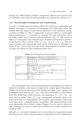
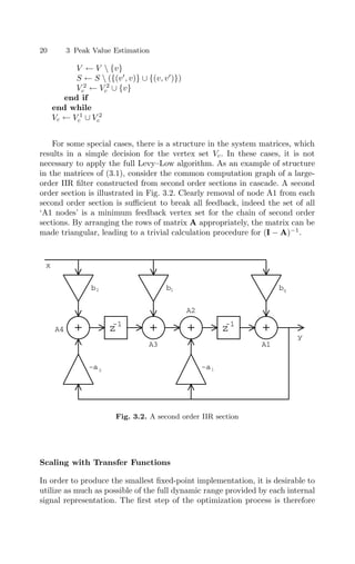
![4.1 Error Estimation 31
S
S
...
...
p’=0
p=-2
j
j
n
nq
q’
j
j
Fig. 4.2. Word-Length and Scaling adjustment
(8,0)
y[t]
-1.6
peak=0.6
(8,0)
(8,0)
+
(8,1)
w[t]
(a) an annotated computation graph
(8,0)
x[t]
peak=0.6
2.1
+
(8,0)
(8,0)
y[t]
-1.6
(8,0)
peak=0.6
(8,0)
(8,1)
-1.8
+
(8,1)
(8,2)
(8,0)
(8,0)
+
(8,2)
(8,2)
(8,1)
(8,1)
q[t]
w[t]
Q
(9,1)
Q
(16,1)
Q
(16,2)
Q
(15,0)
Q
(9,1)
(b) adjusted propagated wordlengths n and quantizers Q explicitly shown
(8,0)
x[t]
peak=0.6
2.1
+
(8,0)
(8,0)
(8,0)
(8,1)
-1.8
+
(8,1)
(8,2)
(8,2)
(8,1)
q[t]
(8,2)
-1
(8,2)
(8,2)
-1
(8,2)
q
Fig. 4.3. Word-Length propagation through an annotated computation graph](https://image.slidesharecdn.com/optimizationandpreparationprocesses-240125021124-f0b0fb42/85/optimization-and-preparation-processes-pdf-44-320.jpg)
![32 4 Word-Length Optimization
word-length nj2 nj1 + n, then this assignment is sub-optimal, since at most
nj1 + n bits are necessary to represent the result to full precision. Ensuring
that such cases do not arise is referred to as ‘conditioning’ the annotated
computation graph [CCL01b]. Conditioning is an important design step, as it
allows the search space of efficient implementations to be pruned, and ensures
that the most efficient use is made of all bits of each signal. It is now possible
to define a well-conditioned annotated computation graph to be one in which
there are no superfluous bits representing any signal (Definition 4.2).
Definition 4.2. An annotated computation graph G
(V, S, A) with A =
(n, p) is said to be well-conditioned iff nj ≤ nq
j for all j ∈ S.
During word-length optimization, ill-conditioned graphs may occur as in-
termediate structures. An ill-conditioned graph can always be transformed
into an equivalent well-conditioned form in the iterative manner shown in
Algorithm WLCondition.
Algorithm 4.1
Algorithm WLCondition
Input: An annotated computation graph G
(V, S, A)
Output: An annotated computation graph, with well-conditioned word-lengths
and identical behaviour to the input system
begin
Calculate p
j and nq
j for all signals j ∈ S (Table 4.1)
Form nq
j from nq
j , p
j and pj for all signals j ∈ S
while ∃j ∈ S : nq
j nj
Set nj ← nq
j
Update nq
j for all affected signals (Table 4.1)
Re-form nq
j from nq
j , p
j and pj for all affected signals
end while
end
4.1.2 Linear Time-Invariant Systems
We shall first address error estimation for linear time-invariant systems. An
appropriate noise model for truncation of least-significant bits is introduced
below. It is shown that the noise injected through truncation can be analyt-
ically propagated through the system, in order to measure the effect of such
a noise on the system outputs. Finally, the approach is extended in order to
provide detailed spectral information on the noise at system outputs, rather
than simply a signal-to-noise ratio.
Noise Model
A common assumption in DSP design is that signal quantization (rounding
or truncation) occurs only after a multiplication or multiply-accumulate op-
eration. This corresponds to a uniprocessor viewpoint, where the result of](https://image.slidesharecdn.com/optimizationandpreparationprocesses-240125021124-f0b0fb42/85/optimization-and-preparation-processes-pdf-45-320.jpg)
![4.1 Error Estimation 33
an n-bit signal multiplied by an n-bit coefficient needs to be stored in an
n-bit register. The result of such a multiplication is a 2n-bit word, which
must therefore be quantized down to n bits. Considering signal truncation,
the least area-expensive method of quantization [Fio98], the lowest value of
the truncation error in two’s complement with p = 0 is 2−2n
− 2−n
≈ −2−n
and the highest value is 0. It has been observed that values between these
ranges tend to be equally likely to occur in practice, so long as the 2n-bit
signal has sufficient dynamic range [Liu71, OW72]. This observation leads
to the formulation of a uniform distribution model for the noise [OW72], of
variance σ2
= 1
12 2−2n
for the standard normalization of p = 0. It has also
been observed that, under the same conditions, the spectrum of such errors
tends to be white, since there is little correlation between low-order bits over
time even if there is a correlation between high-order bits. Similarly, different
truncations occurring at different points within the implementation structure
tend to be uncorrelated.
When considering a multiple word-length implementation, or alternative
truncation locations, some researchers have opted to carry this model over
to the new implementation style [KS98]. However there are associated inac-
curacies involved in such an approach [CCL99]. Firstly quantizations from n1
bits to n2 bits, where n1 ≈ n2, will suffer in accuracy due to the discret-
ization of the error probability density function. Secondly in such cases the
lower bound on error can no longer be simplified in the preceding manner,
since 2−n2
− 2−n1
≈ −2−n1
no longer holds. Thirdly the multiple outputs
from a branching node may be quantized to different word-lengths; a straight
forward application of the model of [OW72] would not account for the cor-
relations between such quantizations. Although these correlations would not
affect the probability density function, they would cause inaccuracies when
propagating these error signals through to primary system outputs, in the
manner described below.
The first two of these issues may be solved by considering a discrete prob-
ability distribution for the injected error signal. For two’s complement arith-
metic the truncation error injection signal e[t] caused by truncation from
(n1, p) to (n2, p) is bounded by (4.1).
−2p
(2−n2
− 2−n1
) ≤ e[t] ≤ 0 (4.1)
It is assumed that each possible value of e[t] has equal probability, as
discussed above. For two’s complement truncation, there is non-zero mean
E{e[t]} (4.2) and variance σ2
e (4.3).
E{e[t]} = − 1
2n1−n2
2n1−n2 −1
i=0
i · 2p−n1
= −2p−1
(2−n2
− 2−n1
)
(4.2)](https://image.slidesharecdn.com/optimizationandpreparationprocesses-240125021124-f0b0fb42/85/optimization-and-preparation-processes-pdf-46-320.jpg)
![34 4 Word-Length Optimization
σ2
e = 1
2n1−n2
2n1−n2 −1
i=0
(i · 2p−n1
)2
− E2
{e[t]}
= 1
12 22p
(2−2n2
− 2−2n1
)
(4.3)
Note that for n1 n2 and p = 0, (4.3) simplifies to σ2
e ≈ 1
12 2−2n2
which is
the well-known predicted error variance of [OS75] for a model with continuous
probability density function and n1 n2.
A comparison between the error variance model in (4.3) and the standard
model of [OS75] is illustrated in Fig. 4.4(a), showing errors of tens of per-
cent can be obtained by using the standard simplifying assumptions. Shown
in Fig. 4.4(b) is the equivalent plot obtained for a continuous uniform distri-
bution in the range [2−n1
− 2−n2
, 0] rather than [2−n2
, 0], which shows even
further increases in error. It is clear that the discretization of the distribu-
tion around n1 ≈ n2 may have a very significant effect on σ2
e . While in a
uniform word-length implementation this error may not be large enough to
impact on the choice of word-length, multiple word-length systems are much
more sensitive to such errors since finer adjustment of output signal quality
is possible.
0
5
10
15
0
2
4
6
8
10
12
14
16
0
0.05
0.1
0.15
0.2
0.25
0.3
0.35
n2
error
(%)
n1 0
5
10
15
0
5
10
15
20
−0.7
−0.6
−0.5
−0.4
−0.3
−0.2
−0.1
0
n2
error
(%)
n1
(a) (b)
Fig. 4.4. Error surface for (a) Uniform [2−n2
, 0] and (b) Uniform [2−n1
− 2−n2
, 0]
Accuracy is not the only advantage of the proposed discrete model. Con-
sider two chained quantizers, one from (n0, p) to (n1, p), followed by one from
(n1, p) bits to (n2, p) bits, as shown explicitly in Fig. 4.5. Using the error
model of (4.3), the overall error variance injected, assuming zero correlation,
is σ2
e0
+ σ2
e1
= 1
12 22p
(2−2n1
− 2−2n0
+ 2−2n2
− 2−2n1
). This quantity is equal
to σ2
e2
= 1
12 22p
(2−2n2
− 2−2n0
). Therefore the error variance injected by con-
sidering a chain of quantizers is equal to that obtained when modelling the
chain as a single quantizer. This is not the case with either of the continuous
uniform distribution models discussed. The standard model of [OW72] gives
σ2
e0
+σ2
e1
= 1
12 (22(p−n1)
+22(p−n2)
). This is not equal to σ2
e2
= 1
12 22(p−n2)
, and
diverges significantly for n2 ≈ n1. This consistency is another useful advantage
of the proposed truncation model.](https://image.slidesharecdn.com/optimizationandpreparationprocesses-240125021124-f0b0fb42/85/optimization-and-preparation-processes-pdf-47-320.jpg)
![4.1 Error Estimation 35
Q Q
(n ,p)
0 (n ,p)
1 (n ,p)
2
(n ,p)
0 (n ,p)
1 (n ,p)
2
+ +
e [t] e [t]
0 1
Q
(n ,p)
0 (n ,p)
2
(n ,p)
0 (n ,p)
2
+
e [t]
2
(a) Two chained quantizers (a) An equivalent structure
Fig. 4.5. (a) Two chained quantizers and their linearized model and (b) an equi-
valent structure and its linearized model
Noise Propagation and Power Estimation
Given an annotated computation graph G
(V, S, A), it is possible to use the
truncation model described in the previous section to predict the variance of
each injection input. For each signal j ∈ {(v1, v2) ∈ S : type(v1) = fork}
a straight-forward application of (4.3) may be used with n1 = nq
j , n2 =
nj, and p = pj, where nq
j is as defined in Section 4.1.1. Signals emanating
from nodes of fork type must be considered somewhat differently. Fig. 4.6(a)
shows one such annotated fork structure, together with possible noise models
in Figs. 4.6(b) and (c). Either model is valid, however Fig. 4.6(c) has the
advantage that the error signals e0[t], e1[t] and e2[t] show very little correlation
in practice compared to the structure of Fig. 4.6(b). This is due to the overlap
in the low-order bits truncated in Fig. 4.6(b). Therefore the cascaded model is
preferred, in order to maintain the uncorrelated assumption used to propagate
these injected errors to the primary system outputs. Note also that the transfer
function from each injection input is different under the two models. If in
Fig. 4.6(b) the transfer functions from injection error inputs e0[t], e1[t] and
e2[t] to a primary output k are given by t0k(z), t1k(z) and t2k(z), respectively,
then for the model of Fig. 4.6(c), the corresponding transfer functions are
t0k(z) + t1k(z) + t2k(z), t1k(z) + t2k(z) and t2k(z).
By constructing noise sources in this manner for an entire annotated com-
putation graph G
(V, S, A), a set F = {(σ2
p, Rp)} of injection input variances
σ2
p, and their associated transfer function to each primary output Rp(z), can
be constructed. From this set it is possible to predict the nature of the noise
appearing at the system primary outputs, which is the quality metric of im-
portance to the user. Since the noise sources have a white spectrum and are
uncorrelated with each other, it is possible to use L2 scaling to predict the
noise power at the system outputs. The L2-norm of a transfer function H(z)
is defined in Definition 4.3. It can be shown that the noise variance Ek at
output k is given by (4.4).](https://image.slidesharecdn.com/optimizationandpreparationprocesses-240125021124-f0b0fb42/85/optimization-and-preparation-processes-pdf-48-320.jpg)
![36 4 Word-Length Optimization
(9,0) (8,0)
(7,0)
(6,0)
+
+
+
e [t]
e [t]
e [t]
0
1
2
(9,0) (8,0)
(7,0)
(6,0)
+
+
+
e [t]
e [t]
e [t]
0
1
2
(8,0)
(7,0)
(6,0)
(9,0)
(a) a FORK
node (b) injection inputs
at each output
(c) cascaded injection
inputs
3 0
1
2
3 0
1
2
0
3
1
2
Fig. 4.6. Modelling post-fork truncation
Ek =
(σp,Rp)∈F
σ2
pL2
2{Rpk} (4.4)
Definition 4.3. The L2-norm [Jac70] of a transfer function H(z) is given
by (4.5), where Z−1
{·} denotes the inverse z-transform.
L2{H(z)} = 1
2π
π
−π
|H(ejθ
)|2
dθ
1
2
=
∞
n=0
|Z−1
{H(z)}[n]|2
1
2
(4.5)
Noise Spectral Bounds
There are some circumstances in which the SNR is not a sufficient quality
metric. One such circumstance is if the user is especially concerned about
noise in particular frequency bands. Consider, for example, the four output
noise spectra illustrated in Fig. 4.7. All spectra have identical power, how-
ever environments sensitive to noise at roughly half the Nyquist frequency
are unlikely to favour the top-left spectrum. Similarly environments sensitive
to high-frequency or low-frequency noise are unlikely to favour the bottom-
left or top-right spectra, respectively. Under these circumstances it is useful
to explore fixed-point architectures having error spectra bounded by a user
specified spectrum function. The two approaches of noise power and noise
spectrum bounds complement each other, and may be used either together or
separately to guide the word-length optimization procedures to be discussed
in this chapter.
This can be achieved by predicting the entire power spectral density
(PSD). The noise PSD Qk(z) at an output k ∈ V of the algorithm may](https://image.slidesharecdn.com/optimizationandpreparationprocesses-240125021124-f0b0fb42/85/optimization-and-preparation-processes-pdf-49-320.jpg)
![4.1 Error Estimation 37
0 0.2 0.4 0.6 0.8 1
10
−15
10
−10
10
−5
10
0
Noise
power
spectrum
0 0.2 0.4 0.6 0.8 1
10
−15
10
−10
10
−5
10
0
0 0.2 0.4 0.6 0.8 1
10
−15
10
−10
10
−5
10
0
Normalized frequency (Nyquist = 1)
Noise
power
spectrum
0 0.2 0.4 0.6 0.8 1
10
−2
10
−1
10
0
10
1
Normalized frequency (Nyquist = 1)
Fig. 4.7. Some different noise spectra with identical noise power
be estimated using the transfer functions Rpk(z) from each noise source to
the output as in (4.6), since each noise source has a white spectrum.
Qk(z) =
(σp,Rp)∈F
σ2
p|Rpk(z)|2
, (z = ejθ
) (4.6)
Once the noise PSD of a candidate implementation G
(V, S, A) has been
predicted, it is necessary to test whether the implementation satisfies the user-
specified constraints. The proposed procedure tests an upper-bound constraint
|Ck(ejθ
)|2
for Qk(z), defined for all θ ∈ [0, 2π) by a real and rational function
Ck(z). The feasibility requirement can be expressed as (4.7).
Qk(ejθ
) |Ck(ejθ
)|2
, for all θ ∈ [0, π] (4.7)
If there is an output k such that Qk(ej0
) ≥ |Ck(ej0
)|2
or Qk(ejπ
) ≥
|Ck(ejπ
)|2
then clearly (4.7) does not hold and the feasibility test is com-
plete. If neither of these conditions are true, and neither Qk(z) nor Ck(z)
have poles on the unit circle |z| = 1, then we may partition the set [0, π] into
2n + 1 subsets {Θ1 = [0, θ1), Θ2 = [θ1, θ2), . . . , Θ2n+1 = [θ2n, π]} such that
Qk(ejθ
) |Ck(ejθ
)|2
for θ ∈ Θ1 ∪ Θ3 ∪ . . . ∪ Θ2n and Qk(ejθ
) ≥ |Ck(ejθ
)|2
for
θ ∈ Θ2 ∪ Θ4 ∪ . . . ∪ Θ2n−1. Since Qk(z) and Ck(z) have no poles on the unit
circle, it may be deduced that Qk(ejθ1
)−|Ck(ejθ1
)|2
= Qk(ejθ2
)−|Ck(ejθ2
)|2
=
Qk(ejθ2n
) − |Ck(ejθ2n
)|2
= 0, and indeed that Qk(ejθ
) − |Ck(ejθ
)|2
= 0 ⇔ θ =](https://image.slidesharecdn.com/optimizationandpreparationprocesses-240125021124-f0b0fb42/85/optimization-and-preparation-processes-pdf-50-320.jpg)
![38 4 Word-Length Optimization
θi for some 1 ≤ i ≤ 2n and θ ∈ (0, π). Thus the problem of testing (4.7) in the
general case has been reduced to the problem of locating those roots of the
numerator polynomial of Fk(z) = numerator(Qk(z)−|Ck(z)|2
) that lie on the
unit circle. In practice, locating roots can be a computation highly sensitive
to numerical error [Act90]. The proposed approach is therefore to locate those
‘approximate’ roots lying in a small annulus around the unit circle, and then
to test a single value of θ between the arguments of each successive pair of
these roots to complete the feasibility test.
If Qk(z) or Ck(z) have large order, there are well-known problems in loc-
ating roots accurately through polynomial deflation [Act90]. Since only those
roots near the unit-circle need be located, it is proposed to use a proced-
ure based on root moment techniques [Sta98] to overcome these problems.
Root moments may be used to factor the numerator polynomial Fk(z) =
F1
k (z)F0
k (z) into two factors, F1
k (z) containing roots within the annulus of
interest, and F0
k (z) containing all other roots. Once F1
k (z) has been extrac-
ted, Laguerre’s method [PFTV88] may be applied to iteratively locate a
single root z0. The factor (z − z0), (z − z0)(z − z∗
0 ), (z − z0)(z − 1/z0) or
(z −z0)(z −z∗
0)(z −1/z0)(z −1/z∗
0), depending on the location of z0, may then
be divided from the remaining polynomial before continuing with extraction
of the next root.
This test can be used by the word-length optimization procedures de-
scribed in Section 4.4 to detect violation of user-specified spectral constraints,
and help guide the choice of word-length annotation towards a noise spectrum
acceptable to the user.
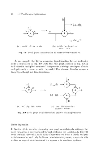
4.1.3 Extending to Nonlinear Systems
With some modification, some of the results from the preceding section can
be carried over to the more general class of nonlinear time-invariant systems
containing only differentiable nonlinearities. In this section we address one
possible approach to this problem, deriving from the type of small-signal ana-
lysis typically used in analogue electronics [SS91].
Perturbation Analysis
In order to make some of the analytical results on error sensitivity for linear,
time-invariant systems [CCL01b] applicable to nonlinear systems, the first step
is to linearize these systems. The assumption is made that the quantization
errors induced by rounding or truncation are sufficiently small not to affect
the macroscopic behaviour of the system. Under such circumstances, each
component in the system can be locally linearized, or replaced by its “small-
signal equivalent” [SS91] in order to determine the output behaviour under a
given rounding scheme.
We shall consider one such n-input component, the differentiable function
Y [t] = f(X1[t], X2[t], . . . , Xn[t]), where t is a time index. If we denote by xi[t]](https://image.slidesharecdn.com/optimizationandpreparationprocesses-240125021124-f0b0fb42/85/optimization-and-preparation-processes-pdf-51-320.jpg)
![4.1 Error Estimation 39
a small perturbation on variable Xi[t], then a first-order Taylor approximation
for the induced perturbation y[t] on Y [t] is given by y[t] ≈ x1[t] ∂f
∂X1
+ . . . +
xn[t] ∂f
∂Xn
.
Note that this approximation is linear in each xi, but that the coeffi-
cients may vary with time index t since in general ∂f
∂Xi
is a function of
X1, X2, . . . , Xn. Thus by applying such an approximation, we have produced
a linear time-varying small-signal model for a nonlinear time-invariant com-
ponent.
The linearity of the resulting model allows us to predict the error at system
outputs due to any scaling of a small perturbation of signal s ∈ S analytically,
given the simulation-obtained error of a single such perturbation instance at
s. Thus the proposed method can be considered to be a hybrid analytic /
simulation error analysis.
Simulation is performed at several stages of the analysis, as detailed be-
low. In each case, it is possible to take advantage of the static schedulability
of the synchronous data-flow [LM87a] model implied by the algorithm repres-
entation, leading to an exceptionally fast simulation compared to event-driven
simulation.
Derivative Monitors
In order to construct the small-signal model, we must first evaluate the differ-
ential coefficients of the Taylor series model for nonlinear components. Like
other procedures described in this section, this is expressed as a graph trans-
formation.
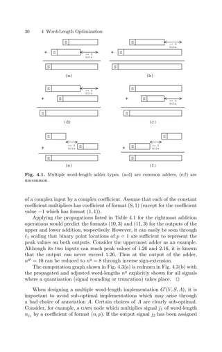
In general, methods must be introduced to calculate the differential of each
nonlinear node type. This is performed by applying a graph transformation to
the DFG, introducing the necessary extra nodes and outputs to calculate this
differential. The general multiplier is the only nonlinear component considered
explicitly in this section, although the approach is general; the graph trans-
formation for multipliers is illustrated in Fig. 4.8. Since f(X1, X2) = X1X2,
∂f
∂X1
= X2 and ∂f
∂X2
= X1.
After insertion of the monitors, a (double-precision floating point) simula-
tion may be performed to write-out the derivatives to appropriate data files
to be used by the linearization process, to be described below.
Linearization
The construction of the small-signal model may now proceed, again through
graph transformation. All linear components (adder, constant-coefficient mul-
tiplier, fork, delay, primary input, primary output) remain unchanged as a
result of the linearization process. Each nonlinear component is replaced by
its Taylor model. Additional primary inputs are added to the DFG to read
the Taylor coefficients from the derivative monitor files created by the above
large-signal simulation.](https://image.slidesharecdn.com/optimizationandpreparationprocesses-240125021124-f0b0fb42/85/optimization-and-preparation-processes-pdf-52-320.jpg)
![4.1 Error Estimation 41
Since the small-signal model is linear, if an output exhibits variance V
when excited by an error of variance σ2
injected into any given signal, then
the output will exhibit variance αV when excited by a signal of variance ασ2
injected into the same signal (0 α ∈ R). Herein lies the strength of the
proposed linearization procedure: if the output response to a noise of known
variance can be determined once only through simulation, this response can be
scaled with analytically derived coefficients in order to estimate the response
to any rounding or truncation scheme.
Thus the next step of the procedure is to transform the graph through the
introduction of an additional adder node, and associated signals, and then
simulate the graph with a known noise. In our case, to simulate truncation of
a two’s complement signal, the noise is independent and identically distributed
with a uniform distribution over the range [−2
√
3, 0]. This range is chosen to
have unit variance, thus making the measured output response an unscaled
‘sensitivity’ measure.
The graph transformation of inserting a noise injection is shown in
Fig. 4.10. One of these transformations is applied to a distinct copy of the
linearized graph for each signal in the DFG, after which zeros are propagated
from the original primary-inputs, to finalize the small-signal model. This is
a special case of constant propagation [ASU86] which leads to significantly
faster simulation results for nontrivial DFGs.
+
a
a
noise
(a) original
signal
(b) with noise
injection
Fig. 4.10. Local graph transformation to inject perturbations
The entire process is illustrated for a simple DFG in Fig. 4.11. The ori-
ginal DFG is illustrated in Fig. 4.11(a). The perturbation analysis will be
performed for the signals marked (*) and (**) in this figure. After inserting
derivative monitors for nonlinear components, the transformed DFG is shown
in Fig. 4.11(b). The linearized DFG is shown in Fig. 4.11(c), and its two
variants for the signals (*) and (**) are illustrated in Figs. 4.11(d) and (e) re-
spectively. Finally, the corresponding simplified DFGs after zero-propagation
are shown in Figs. 4.11(f) and (g) respectively.](https://image.slidesharecdn.com/optimizationandpreparationprocesses-240125021124-f0b0fb42/85/optimization-and-preparation-processes-pdf-54-320.jpg)
![42 4 Word-Length Optimization
*
z-1
X Y
(*) (**)
dc_db
dc_da
*
z-1
X Y
(*) (**)
a
b
c
*
z-1
x
y
(**)
dc_da
(*)
+
*
dc_db
*
z-1
x
y
dc_da
+
*
dc_db
+
noise
z-1
y
*
dc_db +
noise
*
z-1
x
y
dc_da
+
*
dc_db
+
noise
y
noise
(a)
(b) (c)
(d) (e)
(f) (g)
(*)
(**)
Fig. 4.11. Example perturbation analysis
4.2 Area Models
In order to implement a multiple word-length system, component libraries
must be created to support multiple word-length arithmetic. These librar-
ies can then be instantiated by the synthesis system to create synthesizable
hardware description language, and must be modelled in terms of area con-
sumption in order to provide the word-length optimization procedure with a
cost metric.
Since an available target platform for Synthesis is the Altera-based SONIC
reconfigurable computer [HSCL00], these component libraries have been built
from existing Altera macros [Alt98]. Altera provides parameterizable macros
for standard arithmetic functions operating on integer arithmetic, which form
the basis of the multiple word-length libraries for the two arithmetic functions](https://image.slidesharecdn.com/optimizationandpreparationprocesses-240125021124-f0b0fb42/85/optimization-and-preparation-processes-pdf-55-320.jpg)
![4.2 Area Models 43
of constant coefficient multiplication and addition. Integer arithmetic libraries
are also available from many other FPGA vendors and ASIC library suppli-
ers [Xil03, DW]. Multiple word-length libraries have also been constructed
from the Synopsys DesignWare [DW] integer arithmetic libraries, for use in
ASIC designs. Blocks from each of these vendors may have slightly different
cost parameters, but the general approach described in this section is applic-
able across all vendors. The external interfaces of the two multiple word-length
library blocks for gain and add are shown below in VHDL format [IEE99].
ENTITY gain IS
GENERIC( INWIDTH, OUTWIDTH, NULLMSBS, COEFWIDTH : INTEGER;
COEF : std_logic_vector( COEFWIDTH downto 0 ) );
PORT( data : IN std_logic_vector( INWIDTH downto 0 );
result : OUT std_logic_vector( OUTWIDTH downto 0 ) );
END gain;
ENTITY add IS
GENERIC( AWIDTH, BWIDTH, BSHL, OUTWIDTH, NULLMSBS : INTEGER );
PORT( dataa : IN std_logic_vector( AWIDTH downto 0 );
datab : IN std_logic_vector( BWIDTH downto 0 );
result : OUT std_logic_vector( OUTWIDTH downto 0 ) );
END add;
As well as individually parameterizable word-length for each input and
output port, each library block has a NULLMSBS parameter which indicates
how many most significant bits (MSBs) of the operation result are to be ig-
nored (inverse sign extended). Thus each operation result can be considered to
be made up of zero or more MSBs which are ignored, followed by one or more
data bits, followed by zero or more least significant bits (LSBs) which may be
truncated, depending on the OUTWIDTH parameter. For the adder library block,
there is an additional BSHL generic which accounts for the alignment necessary
for addition operands. BSHL represents the number of bits by which the datab
input must conceptually be shifted left in order to align it with the dataa
input. Note that since this is fixed-point arithmetic, there is no physical shift-
ing involved; the data is simply aligned in a skew manner following Fig. 4.1.
dataa and datab are permuted such that BSHL is always non-negative.
Each of the library block parameters has an impact on the area resources
consumed by the overall system implementation. It is assumed, when con-
structing a cost model, both that a dedicated resource binding is to be
used [DeM94], and that the area cost of wiring is negligible, i.e. the designs
are resource dominated [DeM94]. A dedicated resource binding is one in which
each computation node maps to a physically distinct library element. This as-
sumption (relaxed in Chapter 6) simplifies the construction of an area cost
model. It is sufficient to estimate separately the area consumed by each com-
putation node, and then sum the resulting estimates. Of course in reality the
logic synthesis, performed after word-length optimization, is likely to result](https://image.slidesharecdn.com/optimizationandpreparationprocesses-240125021124-f0b0fb42/85/optimization-and-preparation-processes-pdf-56-320.jpg)
![44 4 Word-Length Optimization
in some logic optimization between the boundaries of two connected library
elements, resulting in lower area. Experience shows that these deviations from
the area model are small, and tend to cancel each other out in large systems,
resulting in simply a proportionally slightly smaller area than predicted.
It is extremely computationally intensive to perform logic synthesis each
time an area metric is required for feedback into word-length cost estimation in
optimization. It therefore is advisable to model the area consumption of each
library element at a high level of abstraction using simple cost models which
may be evaluated many times during word-length optimization with little
computational cost. The remainder of this section examines the construction
of these cost models.
The area model for a multiple word-length adder is reasonably straight for-
ward. The ripple-carry architecture is used [Hwa79] since FPGAs provide good
support for fast ripple-carry implementations [Alt98, Xil03]. The only area-
consuming component is the core (integer) adder constructed from the vendor
library. This adder has a width of max(AWIDTH−BSHL, BWIDTH)−NULLMSBS+2
bits. Each bit may not consume the same area, however, because some bits are
required for the result port, whereas others may only be needed for carry
propagation; their sum outputs remain unconnected and therefore the sum
circuitry will be optimized away by logic synthesis. The cost model therefore
has two parameters k1 and k2, corresponding to the area cost of a sum-and-
carry full adder, and the area cost of a carry-only full adder respectively. The
area of an adder is expressed in (4.8).
Aadd(AWIDTH, BWIDTH, BSHL, NULLMSBS, OUTWIDTH) = k1(OUTWIDTH + 1)+
k2(max(AWIDTH − BSHL, BWIDTH) − NULLMSBS − OUTWIDTH + 1)
(4.8)
Area estimation for constant coefficient multipliers is significantly more
problematic. A constant coefficient multiplier is typically implemented as a
series of additions, through a recoding scheme such as the classic Booth tech-
nique [Boo51]. This implementation style causes the area consumption to be
highly dependent on coefficient value. In addition, the exact implementation
scheme used by the vendor integer arithmetic libraries is known only to the
vendor. Although an ideal area model would account for any recoding-based
implementation, this currently remains unimplemented. Instead a simple area
model has been constructed (4.9) and the coefficient values k1 and k2 have
been determined through the synthesis of several hundred multipliers of dif-
ferent coefficient value and width. The model has then been fitted to these
data using a least-squares approach. Note that the model does not account
for NULLMSBS because for a properly scaled coefficient, NULLMSBS ≤ 1 for a
gain block, and therefore has little impact on area consumption.](https://image.slidesharecdn.com/optimizationandpreparationprocesses-240125021124-f0b0fb42/85/optimization-and-preparation-processes-pdf-57-320.jpg)
![4.3 Problem Definition and Analysis 45
Again(INWIDTH, OUTWIDTH, COEFWIDTH) = k3COEFWIDTH(INWIDTH + 1)+
k4(INWIDTH + COEFWIDTH − OUTWIDTH)
(4.9)
4.3 Problem Definition and Analysis
Given a computation graph G(V, S), Chapter 3 has described how a scaling
vector p may be derived. Combining the area models presented in Section 4.2
into a single area measure on G gives a cost metric AG(n, p). Combining the
error variance model (Section 4.1) into a vector EG(n, p), with one element
per output, allows the word-length optimization problem to be formulated as
below. Here E denotes the user specified bounds on error variance.
Problem 4.4 (WORD-LENGTH OPTIMIZATION). Given a compu-
tation graph G(V, S), the word-length optimization problem may be
defined as to select n such that AG(n, p) is minimized subject to (4.10).
n ∈ N|S|
EG(n, p) ≤ E
(4.10)
4.3.1 Convexity and Monotonicity
In this section some results are presented on the nature of the constraint space
defined by (4.10). It is demonstrated that the error observable at primary sys-
tem outputs may not be a monotonically decreasing function in each internal
word-length. Moreover it is illustrated that error non-convexity may occur,
causing the constraint space to be non-convex in n.
It is often generally assumed that the greater the precision to which each
internal variable is known, the greater the precision of the computation out-
put. Indeed Sung and Kum explicitly state this assumption [SK95]. However
a simple example is sufficient to illustrate that to make this assumption for
multiple word-length arithmetic may be fallacious. Consider performing the
operation x = y − y, using possibly different finite precision representations
for the two y values. If the same representation of y is used for both inputs to
the subtraction, then no matter how poor their precision, the result will have
zero error. Using different representations for the two y values will often lead
to a finite error value x. Of course this is a contrived example, and in practice
such a calculation would not be performed. However this section illustrates
that such a result is generalizable to practical applications and can lead to
non-convexity in the constraint space.
Let us first consider signals produced by a single output computation
node, which in turn forms the input to a gain node. An example is shown](https://image.slidesharecdn.com/optimizationandpreparationprocesses-240125021124-f0b0fb42/85/optimization-and-preparation-processes-pdf-58-320.jpg)
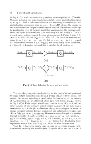
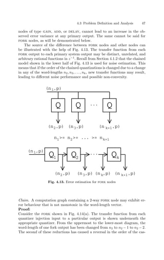
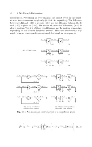
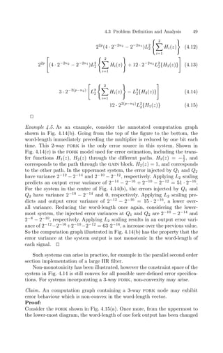
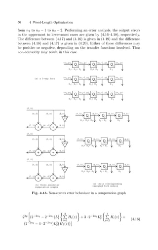
![4.4 Optimization Strategy 1: Heuristic Search 51
22p
(4 · 2−2n2
− 2−2n1
)L2
2
3
i=1
Hi(z)
+ (2−2n3
− 4 · 2−2n2
)L2
2{H3(z)}
(4.17)
22p
(4 · 2−2n2
− 2−2n1
)L2
2
3
i=1
Hi(z)
+ 12 · 2−n2
L2
2{H1(z) + H3(z)}+
(2−2n3
− 16 · 2−2n2
)L2
2{H3(z)}
(4.18)
3 · 22(p−n2)
L2
2
3
i=1
Hi(z)
− L2
2
3
i=2
Hi(z)
(4.19)
12 · 22(p−n2)
L2
2{H1(z) + H3(z)} − L2
2{H3(z)}
(4.20)
Example 4.6. As an example, consider the annotated computation graphs
shown in Fig. 4.15(b). In the uppermost graph, the errors injected by quant-
izers Q1, Q2 and Q3 have variance 2−12
− 2−14
, 2−10
− 2−12
and 2−8
− 2−10
,
respectively. Applying L2 scaling results in a predicted error variance of
25 · (2−16
− 2−18
) + 2−14
− 2−16
+ 9 · (2−12
− 2−14
) = 519 · 2−18
. For the
system in the centre of Fig. 4.15(b), the errors injected by quantizers Q1, Q2
and Q3 have variance 2−10
− 2−14
, 0, and 2−8
− 2−10
, respectively. Apply-
ing L2 scaling results in a predicted error variance of 25 · (2−14
− 2−18
) +
9 · (2−12
− 2−14
) = 807 · 2−18
, an increase on the previous error variance.
Finally considering the lower-most system in Fig. 4.15(b), the errors injec-
ted by quantizers Q1, Q2 and Q3 have variance 2−10
− 2−14
, 2−8
− 2−10
and
0, respectively. Applying L2 scaling results in a predicted error variance of
25 · (2−14
− 2−18
) + 2−12
− 2−14
= 423 · 2−18
, a reduction over the previous
error variance. Thus if a user-specified constraint on the output noise power
were set between 519·2−18
and 807·2−18
, then the uppermost and lower-most
structures would be feasible but the centre structure would be infeasible.
It has been shown that the noise model derived in Section 4.1.2 leads to a
constraint space which, under well defined conditions, may be non-convex in
the word-length optimization variables. It should be noted that this property
is not simply an artifact of the noise model, but has been observed in practice
using bit-true simulation. This non-convexity makes the constraint space a
harder space to search for optimum solutions [Fle81].
4.4 Optimization Strategy 1: Heuristic Search
Since the word-length optimization problem is NP-hard [CW01], a heuristic
approach has been developed to find feasible word-length vectors having small,](https://image.slidesharecdn.com/optimizationandpreparationprocesses-240125021124-f0b0fb42/85/optimization-and-preparation-processes-pdf-64-320.jpg)
![52 4 Word-Length Optimization
though not necessarily optimal, area consumption. The heuristic algorithm
used is shown in Algorithm Word-LengthFalling. After performing an 1 scal-
ing, the algorithm determines the minimum uniform word-length satisfying
all error constraints. The design at this stage corresponds to a standard uni-
form word-length design with implicit power-of-two scaling, such as may be
used for an optimized uniprocessor-based implementation. Each word-length
is then scaled up by a factor k 1, which represents a bound on the largest
value that any word-length in the final design may reach. In the Synoptix
implementation [CCL00a, CCL01b], k = 2 has been used. At this point the
structure may be ill-conditioned, requiring reduction to a well-conditioned
structure, as described in Section 4.1.1.
The resulting well-conditioned structure forms a starting point from which
one signal word-length is reduced by one bit on each iteration. The signal
word-length to reduce is decided in each iteration by reducing each word-
length in turn until it violates an output noise constraint. At this point there
is likely to have been some pay-off in reduced area, and the signal whose
word-length reduction provided the largest pay-off is chosen. Each signal’s
word-length is explored using a binary search.
Although Algorithm Word-LengthFalling is a greedy algorithm, both the
constraints and the objective function play a role in determining the direction
of movement towards the solution. As a result, this algorithm is less dependent
on local information than a pure steepest-descent search.
Algorithm 4.2
Algorithm Word-LengthFalling
Input: A Computation Graph G(V, S)
Output: An optimized annotated computation
graph G
(V, S, A), with A = (n, p)
begin
Let the elements of S be denoted as S = {j1, j2, . . . j|S|}
Determine p through 1 scaling
Determine u, the minimum uniform word-length satisfying (4.10)
with n = u · 1
Set n ← ku · 1
do
Condition the graph G
(V, S, A)
Set currentcost ← AG(n, p)
foreach signal ji ∈ S do
Set bestmin ← currentcost
Determine w ∈ {2, . . . , nji }, if such a w exists, such
that (4.10) is satisfied for annotation ([nj1 . . . nji−1 w nji+1 . . . nj|S|
]T
, p)
but not satisfied for annotation ([nj1 . . . nji−1 (w − 1) nji+1 . . . nj|S|
]T
, p)
If such a w exists, set minval ← AG([nj1 . . . nji−1 w nji+1 . . . nj|S|
]T
, p)
If no such w exists, set minval ← AG([nj1 . . . nji−1 1 nji+1 . . . nj|S|
]T
, p)
if minval bestmin do](https://image.slidesharecdn.com/optimizationandpreparationprocesses-240125021124-f0b0fb42/85/optimization-and-preparation-processes-pdf-65-320.jpg)
![4.5 Optimization Strategy 2: Optimum Solutions 53
Set bestsig ← j, bestmin ← minval
end if
end foreach
if bestmin currentcost
nbestsig ← nbestsig − 1
while bestmin currentcost
end
Algorithm Word-LengthFalling will, in general, provide better results un-
der a convex constraint space. However the non-convexities described in Sec-
tion 4.3.1 should not affect its operation too severely. The binary search mech-
anism will result in ‘jumping over’ infeasible portions of non-convex constraint
space in some cases, and will remain stuck on one side of an infeasible region
in other cases. In either case, since the word-lengths are only reduced by one
bit each time, the next iteration will be facing the non-convexity from a differ-
ent direction. Non-convexity can manifest itself in intermediate word-length
vectors having infeasible error properties. However the final word-length vec-
tor will always be feasible, as moves are only ever performed in a direction
leading to a feasible solution and the cost metric AG(n, p) is monotonic in n.
The overwhelming proportion of execution time in Algorithm Word-
LengthFalling is spent in the iterative refinement of the initial scaled-up uni-
form word-length solution. The average-case execution time will be discussed
in Section 4.6.1.
4.5 Optimization Strategy 2: Optimum Solutions
The contribution of section is to present a technique for optimum word-length
allocation, for the case where the DSP algorithm to be synthesized is a linear,
time-invariant (LTI) system [Mit98].
The Mixed Integer Linear Programming (MILP) technique described in
this section has been applied to several small benchmark circuits, and the res-
ults compared to the heuristic presented in Section 4.4. Modelling as a MILP
permits the use of industrial-strength MILP solvers such as BonsaiG [Haf].
Although MILP solution time can render the synthesis of large circuits in-
tractable, optimal results even on small circuits are valuable as benchmarks
with which to compare heuristic optimization procedures.
The proposed MILP model contains several variables, which may be clas-
sified as: integer signal word-lengths and signal word-lengths before quantiz-
ation, binary auxiliary signal word-lengths and auxiliary signal word-lengths
before quantization, binary decision variables, real adder costs, and real fork
node errors.
Note that only adders, gains, and delays cost area resources (forks are
considered free). However adders have an inherently complex area model and](https://image.slidesharecdn.com/optimizationandpreparationprocesses-240125021124-f0b0fb42/85/optimization-and-preparation-processes-pdf-66-320.jpg)
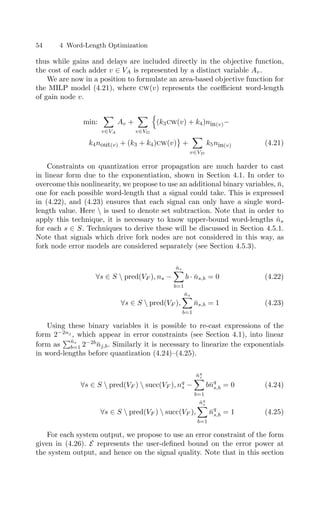
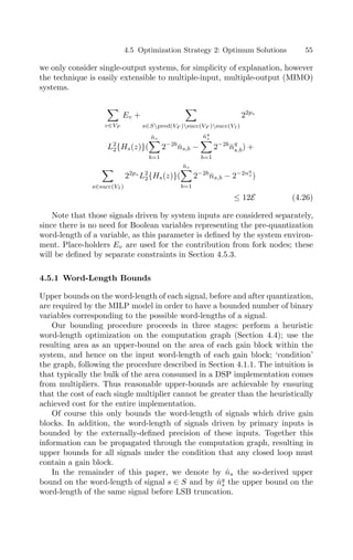
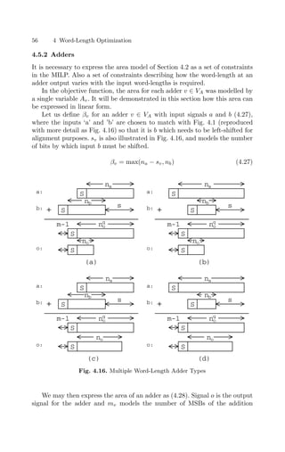
![4.5 Optimization Strategy 2: Optimum Solutions 57
which are known through scaling to contain no information, as described in
Chapter 3 and illustrated in Fig. 4.1. This value is independent of the word-
lengths, and for an adder can be expressed as mv = max(pa, pb) + 1 − po.
Av =
k1(no + 1) + k2 [β − mv − no + 1] ,
no + mv ≤ β + 1
k1 [β − mv + 2] ,
otherwise
(4.28)
The non-linearities due to the max operator in (4.27) and the decision
in (4.28) must be linearized for the MILP model. This is achieved through
the introduction of four binary decision variables δv1, δv2, δv3 and δv4 for each
adder v ∈ VA.
For the remainder of this section, we consider a general adder with inputs
i and j and output o, to distinguish from the more specific case considered
above, where input b was used to denote the left-shifted input to an adder.
In order to model (4.27), if pj ≤ pi then (4.29)–(4.32) are included in the
MILP. Otherwise (4.33)–(4.36) are included in the MILP. The right-hand side
of each inequality consists of a trivial bound on the left-hand side, multiplied
by a decision variable.
ni − nj + pj − pi δv1(n̂i + pj − pi) (4.29)
βv − nj + pj − pi ≥ (1 − δv1)(−n̂j − pi + pj) (4.30)
ni − nj + pj − pi ≥ δv2(−n̂j + pj − pi) (4.31)
βv − ni ≥ (1 − δv2)(−n̂i) (4.32)
nj − ni + pi − pj δv1(n̂j − pj + pi) (4.33)
βv − ni + pi − pj ≥ (1 − δv1)(1 − n̂i − pj + pi) (4.34)
nj − ni + pi − pj ≥ δv2(−n̂i + pi − pj) (4.35)
βv − nj ≥ (1 − δv2)(−n̂j) (4.36)
Note that βv and αv are only bounded from below by the constraints given.
Inequalities are used in order to allow disjunctions and thus implications, for
example selecting δv1 = 0 in (4.29) gives ni−nj +pj −pi 0, whereas selecting
δv1 = 1 gives βv − nj + pj − pi ≥ 0. Allowing δv1 as an optimization variable
results in ni ≥ nj − pj + pi ⇒ βv ≥ nj + pj − pi. Equality of Av is guaranteed
through its positive coefficient in the objective function.
In order to model (4.28), (4.37)–(4.40) are included in the MILP. These
terms model the choice in (4.28) as a pair of implications, in an identical
manner to that described above.](https://image.slidesharecdn.com/optimizationandpreparationprocesses-240125021124-f0b0fb42/85/optimization-and-preparation-processes-pdf-70-320.jpg)
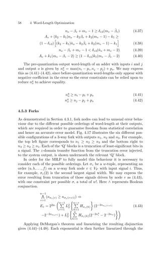
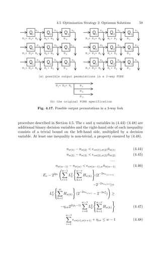
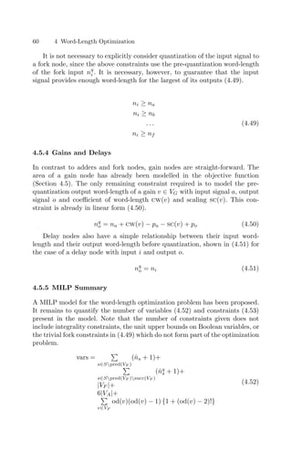
![4.6 Some Results 61
cons = 2|S pred(VF )|+
2|S pred(VF ) succ(VF )|+
1+
10|VA|+
v∈VF
od(v)(od(v) − 1) {1 + 2(od(v) − 2)!} +
|VG| + |VD|
(4.53)
It can be seen that so long as the number of large-fanout fork nodes are
limited, the number of constraints in the MILP model grows approximately
linearly in the number of nodes and signals. Under the same conditions the
number of variables can grow up to quadratically with the number of signals
because the upper bounds on each signal word-length will vary approximately
linearly with the number of large area-consuming nodes. Both parameters are
dominated by any large-fanout fork nodes, since the number of η variables
and their associated constraints grow combinatorially with fanout.
4.6 Some Results
Synoptix, a complete synthesis system incorporating the algorithms in this
chapter, has been developed for implementation of multiple word-length sys-
tems in FPGAs. The input to Synoptix is a Simulink [SIM] block diagram,
and the output is a structural description in VHDL [IEE99] or AHDL [MAX].
FPGA vendor tools are then used to perform the low-level logic synthesis,
placement, and routing of the designs. The design-flow for implementation on
the Sonic platform [HSCL00] is illustrated in Fig. 4.18, with the Sonic-specific
parts shaded.
signal
scaling
wordlength
optimization
Simulink
error
constraints
synthesis of
HDL
vendor
synthesis
completed
design
bit-true
simulator
HDL
libraries
library
cost models
multiple
wordlength
libraries
Fig. 4.18. Synoptix design flow](https://image.slidesharecdn.com/optimizationandpreparationprocesses-240125021124-f0b0fb42/85/optimization-and-preparation-processes-pdf-74-320.jpg)
![62 4 Word-Length Optimization
The system has been tested on several benchmark circuits, including fi-
nite impulse response (FIR) and infinite impulse response (IIR) filters, a dis-
crete cosine transform (DCT), a polyphase filter bank (PFB), and an RGB
to YCrCb convertor. It is important to note that all results presented in this
section are measured from placed and routed designs, rather than estimated
from the library cost estimation procedure described in Section 4.2.
4.6.1 Linear Time-Invariant Systems
Mixed Integer Linear Programming Results
Fig. 4.19 illustrates area-error tradeoff curves for both a second and a third
order linear phase FIR filter [Mit98]. For the second order filter, results for
both 4-bit and 8-bit inputs are given. For the third order filter, only results
for a 4-bit input have been obtained. Three curves are present in each plot:
the optimum uniform word-length implementation, the heuristically derived
multiple word-length implementation from (Section 4.4), and the optimum
multiple word-length implementation achieved by solving the MILP presented
in Section 4.5.
10
−8
10
−7
10
−6
10
−5
10
−4
10
−3
10
−2
10
−1
0
20
40
60
80
100
120
140
2nd order, 4−bit input, optimum
2nd order, 4−bit input, heuristic
2nd order, 4−bit input, uniform
3rd order, 4−bit input, optimum
3rd order, 4−bit input, heuristic
3rd order, 4−bit input, uniform
2nd order, 8−bit input, optimum
2nd order, 8−bit input, heuristic
2nd order, 8−bit input, uniform
Area
(4LUTs)
Error variance specification
Fig. 4.19. Area / Error tradeoffs compared for a 2nd and 3rd order FIR filter
The results clearly illustrate the high-quality solutions achievable by the
heuristic solution, averaging only 0.7% with a maximum of 3.9% worse than
the optimum result.
An optimum word-length allocation for an RGB to YCrCb convertor with
4-bit inputs has also been performed. This result shows an optimal cost of
78.61 LUTs, equal to the result achieved by the heuristic.](https://image.slidesharecdn.com/optimizationandpreparationprocesses-240125021124-f0b0fb42/85/optimization-and-preparation-processes-pdf-75-320.jpg)
![4.6 Some Results 63
Fig. 4.20 illustrates the structure [Eva] and optimum word-lengths of the
RGB to YCrCb converter for 4-bit inputs (of range ±112), 4-bit coefficients,
and with an error-free Y, whereas a bounded error power of up to 10−2
has
been allowed for Cr and Cb.
+
+
+
+
r
g
b
Y
Cr
Cb
4 4
4
4
4
4
4
6
6 10 10
10
10
10
10
11
10
10
10
6
8
Fig. 4.20. Optimal word-length allocations for the ITU RGB to YCrYb converter
The BonsaiG MILP solver [Haf] was used to solve the MILP models: exe-
cution time ranged from 2 seconds to 6 minutes on an AMD Athlon 1.2 GHz
with 512 MB RAM. This compares to less than 0.2 second for the heuristic
solutions on the same machine. Limits on the scale of the MILP solvable are
due to both excessive run-time and numerical instabilities in the MILP solver.
Heuristic Results
Shown in Fig. 4.21 is a graph of placed-and-routed resource usage (measured
in Altera Flex10k logic cells [Alt98]) against specified error variance. This
plot is representative in terms of the general shape of the plots obtained
for all designs. The benchmark is a simple second order (biquadratic) IIR
digital filter. Both the multiple word-length design and the optimized uniform
word-length structure are shown. The plot of area for a uniform word-length
decreases in steep steps. This is because there is a sudden change when the
next-lowest word-length becomes feasible with respect to the error constraints.
This is not the case for the optimized multiple word-length structures, since
there are many more optimization variables and hence many different error
powers are achievable. In addition, the heuristic line lies consistently below
the uniform line (by 2% to 15%), showing a consistent area saving for this
design.](https://image.slidesharecdn.com/optimizationandpreparationprocesses-240125021124-f0b0fb42/85/optimization-and-preparation-processes-pdf-76-320.jpg)
![64 4 Word-Length Optimization
10
0
10
1
360
380
400
420
440
460
480
500
520
540
error variance specification
No.
logic
cells
uniform wordlength
optimized multiple wordlength
Fig. 4.21. Circuit area against specified error power for an IIR biquadratic filter
Table 4.2 illustrates some further results from larger benchmark circuits.
Both the number of logic cells (LCs) and maximum clock frequency are re-
ported. Each of these results corresponds to a single point on the area-error
tradeoff curve for the circuit, and have been placed and routed in an Altera
Flex10k70RC240-3 device (as used in the Sonic [HSCL00] platform) except
where otherwise stated. The FIR filter is a 126-tap linear-phase low-pass Dir-
ect Form II transposed [Mit98] structure, suggested by [LKHP97] as a rep-
resentative DSP design. The DCT is an 8-point, 1-dimensional decimation in
time structure from [Par99] which has also been suggested as a benchmark
by [LKHP97]. Two versions of this benchmark have been synthesized, one
(DCT1
) with equal error tolerance on all outputs, and the other (DCT2
) with
required signal-to-noise ratio (SNR) reducing by 3dB per DCT coefficient,
so that low frequency coefficients are less noisy than high-frequency ones.
The IIR filter is of 4th order, as used by [KKS00] and is of interest since it
has a recursive (feedback) structure. The polyphase filter bank (PFB) is the
design given in [FGL01] for evaluation of the Streams-C compiler. The RGB
to YCrCb convertor is of the form suggested by the ITU [Eva], and allows
some quantization error in the Cr and Cb outputs whereas the Y output is
guaranteed to be error-free. This design is of particular interest since the mul-
tiple word-length approach can clearly be used to customize the datapath in
order to achieve these differential specifications. Each of these circuits has](https://image.slidesharecdn.com/optimizationandpreparationprocesses-240125021124-f0b0fb42/85/optimization-and-preparation-processes-pdf-77-320.jpg)
![4.6 Some Results 65
been synthesized twice, once using an optimal uniform word-length structure,
and once using the multiple word-length structure generated by the Synop-
tix tool. The DCT designs have been synthesized on a device with a larger
number of I/O pins, due to the I/O-limited nature of the designs, whereas the
FIR filter has been synthesized on a device with a significantly larger logic
capacity.
Table 4.2. Lossy synthesis results
Design Uniform wl
Area (#LCs) fclk (MHz) width (bits)
FIR†
6125 29.15 16
DCT1∗
1394 12.95 13
DCT2∗
1367 13.03 12
IIR 701 9.57 12
PFB 321 30.03 15
RGB–YCrCb 438 11.58 18
Design Multiple wl
Area (#LCs) % improvement fclk (MHz) % improvement
FIR†
3356 42.5% 36.23 2.5%
DCT1∗
1311 6.0% 13.67 5.6%
DCT2∗
1164 14.9% 13.53 3.8%
IIR 623 11.1% 9.32 -2.6%
PFB 273 15.0% 31.34 4.4%
RGB–YCrCb 272 37.9% 16.15 39.5%
∗
implemented on Flex10k70GC503-3
†
implemented on Flex10k200SRC240-1
It should be noted that even for the uniform word-length structures, Syn-
optix has been used to automatically insert power-of-two scaling [Jac70], which
is good practice in DSP design. Also note that for both uniform and multiple
word-length structures, these circuits represent a completely unpipelined im-
plementation of the specification, in order to aid direct comparison of max-
imum clock rate fclk reported.
Table 4.2 illustrates that area reductions of between 6% and 45% (mean
22%) have been achieved by using the multiple-word-length synthesis ap-
proach described in this chapter. These area reductions have been accompan-
ied by a speedup in maximum clock frequency between −3% and 39% (mean
12%), even though the estimated speed is not considered by the cost function
used for optimization. Interestingly, the only benchmark to have been slowed
down slightly as a result of the optimization is the IIR filter. This is due to the
increase of some signal word-lengths on the critical path around the feedback
loops in this filter. Importantly, the largest area reductions and speedups have
occurred in both the FIR filter, which is the largest design shown, and the
RGB to YCrCb convertor, which has a structure ideally suited to multiple](https://image.slidesharecdn.com/optimizationandpreparationprocesses-240125021124-f0b0fb42/85/optimization-and-preparation-processes-pdf-78-320.jpg)
![66 4 Word-Length Optimization
word-lengths since the error-free Y is calculated first, from which Cr and Cb
are derived [Eva].
With the exception of the IIR filter, all benchmarks have also been syn-
thesized with a specification of zero error. This is a degenerate case of the
optimization procedure, corresponding to lossless synthesis, and has been per-
formed to enable possible comparisons with other lossless approaches. (Note
that the IIR filter cannot be synthesized in a lossless way due to the feedback.)
Table 4.3 illustrates these results. The FIR result for area is only an estimate
reported by the synthesis tools since the design was unable to be placed in the
largest device supported by Altera MaxPlusII, and for the same reason there
is no clock frequency result for this benchmark under lossless synthesis. The
most important trend to be gleaned from these results is that the correctness
preserving (lossless) approach to high-level synthesis of DSP structures from
floating-point specifications is insufficient by itself to achieve results matching
or improving on traditional DSP design techniques, when some output roun-
doff error can be tolerated. For as long as output error is not considered as a
design variable by high-level synthesis systems, design specification languages
must explicitly consider word-length or sub-optimal designs will often result.
Table 4.3. Lossless synthesis results
Design Multiple wl
Area (#LCs) fclk (MHz)
FIR†
11110 †
DCT∗
1530 12.77
PFB 332 38.31
RGB–YCrCb 547 11.99
∗
implemented on Flex10k70GC503-3
†
design too large for Flex10k200 device
Table 4.4 presents the execution times of an unoptimized C implementa-
tion of Algorithm Word-LengthFalling (without spectral constraints) running
on a Pentium III 450MHz, for each of the benchmark circuits discussed in the
previous section.
In order to provide an insight into the way in which algorithm execution
time scales with the size of the synthesized system, Direct Form II FIR filters
with between 6 and 74 taps have been generated and optimized using the
heuristic from Section 4.4. Fig. 4.22 illustrates the results. Let n be the number
of filter taps. The do–while refinement loop of the algorithm will be executed
a number of times approximately proportional to n, since only one word-length
will be reduced by one bit on each iteration. The foreach statement will be
executed |S| times, which is proportional to n for an FIR filter structure.
Finally the error estimation phase execution time will be generally linear in
n. Overall, the expected average-case execution time is proportional to n3
.](https://image.slidesharecdn.com/optimizationandpreparationprocesses-240125021124-f0b0fb42/85/optimization-and-preparation-processes-pdf-79-320.jpg)
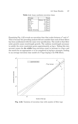
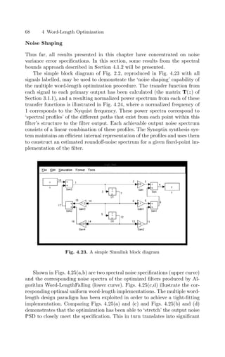
![4.6 Some Results 69
0 0.2 0.4 0.6 0.8 1
10
−1
10
0
10
1
Power
Spectrum
Signals 0,2,4−6,8,11,13
0 0.2 0.4 0.6 0.8 1
10
−3
10
−2
10
−1
10
0
Signals 9,12
0 0.2 0.4 0.6 0.8 1
10
−3
10
−2
10
−1
10
0
Normalized frequency
Power
Spectrum
Signals 3,7
0 0.2 0.4 0.6 0.8 1
10
−10
10
−5
10
0
Normalized frequency
Signals 1,10,14−18
Fig. 4.24. Spectral profiles through the filter
area savings: for this example the uniform word-length design requires 810
logic cells in an Altera Flex10K device, compared to 636 and 663 logic cells
for the shaped designs, a 22% and 18% area reduction respectively.
The spectral specifications are only slightly different in the two cases of
Figs. 4.25(a) and (b): Fig. 4.25(b) has a somewhat reduced bound on high-
frequency noise. The optimization procedure has successfully incorporated the
modified constraint by reducing the high-frequency noise in the implemented
structure. In contrast, there has been no change to the uniform word-length
system between Figs. 4.25(c) and (d), since with a uniform word-length struc-
ture only a limited range of output noise spectra are possible.
4.6.2 Nonlinear Systems
Case Study: Adaptive Filtering
Adaptive filtering is a common DSP application, especially in the field of
communications where it is widely used, for example, to compensate for multi-
path distortion in mobile communication systems [Hay96].
In addition to its practical significance, adaptive filtering has some inter-
esting algorithmic features:
• All adaptive filtering algorithms contain feedback, limiting the applic-
ability of several existing word-length optimization techniques [WP98,](https://image.slidesharecdn.com/optimizationandpreparationprocesses-240125021124-f0b0fb42/85/optimization-and-preparation-processes-pdf-82-320.jpg)
![70 4 Word-Length Optimization
0 0.2 0.4 0.6 0.8 1
10
−7
10
−6
10
−5
10
−4
(a)
Power
Spectrum
0 0.2 0.4 0.6 0.8 1
10
−7
10
−6
10
−5
10
−4
(b)
0 0.2 0.4 0.6 0.8 1
10
−7
10
−6
10
−5
10
−4
(c)
Normalized frequency
Power
Spectrum
0 0.2 0.4 0.6 0.8 1
10
−7
10
−6
10
−5
10
−4
(d)
Normalized frequency
Fig. 4.25. Two specifications (upper curve) and their optimized (a,b) multiple
word-length and (c,d) uniform word-length implementation noise spectra
NHCB01, BP00, SBA00, CRS+
99] and limiting the performance achiev-
able through pipelining.
• Adaptive filters contain general multipliers, rather than the constant coef-
ficient multipliers present in static filters. This means that adaptive filters
are nonlinear systems, limiting the applicability of purely analytic tech-
niques such as that presented in Section 4.1.2 [CCL01b, CCL02].
• The coefficients of an adaptive filter are updated by accumulating (usually
small) correction terms. Such ‘integration loops’ make the outputs of an
adaptive filter very sensitive to errors induced around such loops.
The so-called least-mean-square (LMS) adaptive filter [Hay96] will be con-
sidered in this section, due to its widespread use in practice. For the unfamiliar
reader, a brief review of LMS filters will now be provided.
Consider an input signal x[t] and a desired filter response d[t]. (The desired
response could be known a-priori, for example from a ‘training sequence’ used
in GSM mobile telephony). Let n denote the order of the filter, and u[t] denote
the vector u[t] = (x[t] x[t − 1] x[t − 2] . . . x[t − n])T
, where T
represents
vector/matrix transpose. An LMS filter with real input and coefficients has
the following algorithm, where 0 represents a column vector with each element
equal to 0, and µ is a user-chosen scalar adaptation coefficient.](https://image.slidesharecdn.com/optimizationandpreparationprocesses-240125021124-f0b0fb42/85/optimization-and-preparation-processes-pdf-83-320.jpg)
![4.6 Some Results 71
w[0] = 0
for t ≥ 0 do
y[t] = wT
[t]u[t]
e[t] = d[t] − y[t]
w[t + 1] = w[t] + µu[t]e[t]
end do
A DFG for a first-order LMS filter is shown in Fig. 4.26. The DFG for an
nth order filter is easily derived through a replication of the taps and the use
of an adder-tree to sum the partial results.
+ z-1
F
* *
F z-1
+ z-1
F
* *
F
+
F +
F
x
y
-1
d
filter taps
Fig. 4.26. First order LMS adaptive filter
Area, Power, and Speed
In order to demonstrate the area, power, and delay advantages of the proposed
method, 90 filters of between 1st and 10th order have been constructed and
synthesised. In each case the ‘desired’ input d[t] to the adaptive filter is a well-
known 100,000 sample voice clip from [FRE93]. The filter input x[t] is a version
of the same signal, corrupted by three different 12th order autoregressive
filters, operating on three disjoint and equally sized portions of the input
signal. Each distortion filter has constant coefficients randomly chosen such
that the filter poles occur in complex conjugate pairs and have independent,
identically distributed uniform distribution in magnitude range (0, 1) and in
phase range (0, π/2).
The filter designs and input sequences have then been passed to the syn-
thesis tool, and for each design three different optimization procedures have
been followed. Firstly, the design has been synthesized with the optimum uni-
form scaling and the optimum uniform word-length for all signals. This design
choice reflects the simplest form of optimized DSP design. Secondly, the design
has been synthesized with scaling individually optimized for each signal (see](https://image.slidesharecdn.com/optimizationandpreparationprocesses-240125021124-f0b0fb42/85/optimization-and-preparation-processes-pdf-84-320.jpg)
![72 4 Word-Length Optimization
Chapter 3) and the optimum uniform word-length. This design choice reflects
the use of a tool such as [SBA00] which focuses on optimizing signals from
the MSB-side. The final design procedure has been to use an individually
optimized scaling combined with an individually optimized word-length, as
proposed by this chapter.
From the filter designs in Simulink and the representative input sequences,
the synthesis tool automatically generates a combination of structural VHDL
and Xilinx Coregen scripts, together with a makefile to synthesize the Virtex
bit-stream. Each design has been fully placed and routed in a Xilinx Virtex
1000 (XCV1000BG560-6), after which an area, power consumption, and tim-
ing analysis has been performed. Due to memory and run-time constraints
imposed by large value-change-dump simulation files, power analysis could
only be performed for a 100-sample portion of the 100,000-sample input se-
quence used by the tool.
The first set of results is concerned with the variation of design metrics
with the order of the filter to be synthesized. For each of these results, the
filters have been synthesized using the same lower-bound on output SNR of
34dB.
The results are illustrated in Fig. 4.27(a), (b) and (c) for area, power,
and clock period, respectively. Area savings of up to 37% (mean 32%) have
been achieved over scaling optimization alone, and up to 63% (mean 61%)
over neither scaling nor word-length optimization. This is combined with a
power reduction of up to 49% (mean 43%) and speed-up of up to 18% (mean
10%) over scaling optimization alone, and a power reduction of up to 84.6%
(mean 81.2%) and speed-up of up to 29% (mean 18%) over neither scaling
nor word-length optimization.
The second set of results is concerned with the variation of design metrics
with the user-specified lower-bound on allowable SNR. For these results, a
5th order LMS filter has been synthesized with SNR bound varying between
−6dB and 64dB. These results are illustrated in Fig. 4.28(a), (b) and (c)
for area, power, and clock period, respectively. As well as demonstrating the
useful capability to trade-off numerical accuracy for area, power and speed,
these results also illustrate significant improvements in all three metrics.
Area savings have been achieved of up to 75% (mean 45%) over scaling
optimization alone, and up to 80% (mean 66%) over neither scaling nor word-
length optimization. This is combined with a power reduction of up to 96%
(mean 58%) and speed-up of up to 29% (mean 11%) over scaling optimization
alone, and a power reduction of up 98% (mean 87%) and speed up of up to
36% (mean 20%) over neither scaling nor word-length optimization.
It should be expected that on average the power savings are no smaller than
the area savings of this approach. However in practice, the power savings are
often significantly greater. This can be explained by two observations relating
to the switching activity of signals. Firstly, if the scaling of each signal is
not individually optimized, then a significant number of signals will contain
unnecessary sign-extension. When a two’s complement signal changes from a](https://image.slidesharecdn.com/optimizationandpreparationprocesses-240125021124-f0b0fb42/85/optimization-and-preparation-processes-pdf-85-320.jpg)
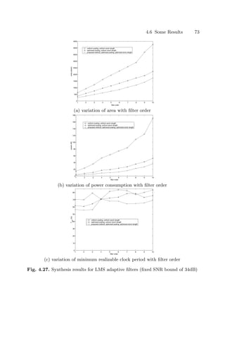
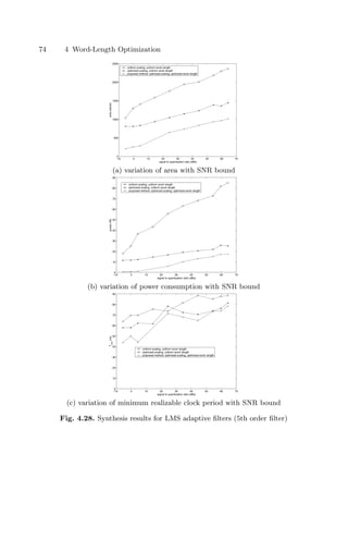
![4.6 Some Results 75
positive to a negative value, or vice-versa, all of these MSBs will toggle. Thus
the overall switching activity in a realization can be reduced dramatically by
applying scaling optimization. Secondly, when a sampled signal is in a period
of relatively low-frequency (with respect to the Nyquist rate), the activity
amongst low-order bits is, on average, likely to be significantly larger than
that amongst high-order bits due to the slowly changing signal value. Thus
word-length optimization, which specifically targets the low-order bits of each
signal, is likely to lead to a significant reduction in the overall activity level.
In addition, it is likely that a large portion of the power consumption due
to logic activity in DSP systems derives from multiplier cores. In multipliers,
the power consumption is far more sensitive to reductions in the switching
activity of low-order input bits than that of high-order input bits [MS01].
These explanations are supported by the plot of Fig. 4.28(b) which shows
the power saving of the proposed method over scaling optimization alone
increasing rapidly for low SNR. This is because the low SNR allows word-
length optimization to aggressively target more low-order bits.
4.6.3 Limit-cycles in Multiple Word-Length Implementations
The multiple word-length design paradigm, combined with a word-length op-
timization technique, has been shown to be highly effective at optimizing
system area for a given user-specified bound on truncation noise. However,
a finite precision implementation can additionally suffer from certain types
of noise not considered in Section 4.1.2. A finite precision implementation of
an IIR filter is essentially a finite state machine (FSM). Under any unchan-
ging input vector, an FSM may exhibit one of two steady-state behaviours:
it may either settle in an ‘attractor state’, or it may cycle around a finite
number of states. The latter of the two behaviours can result in output oscil-
lations in a finite precision implementation, which would not be present for
the infinite precision case. In Digital Signal Processing, this inherently non-
linear behaviour is referred to as limit-cycle behaviour [Mit98]. There have
been several studies into limit cycles [LMV88, BB90, PKBL96], generally fo-
cussing on conditions for non-existence of limit cycles in uniform word-length
implementations, and indentifying regions of the coefficient space guaranteed
to be limit-cycle free. While limit cycle behaviour is not considered by the
optimization procedure developed in this chapter, it is nevertheless important
from a user’s perspective that the limit-cycle behaviour of the optimized mul-
tiple word-length systems is not generally worse than that of more traditional
implementation schemes.
In order to compare the limit-cycle behaviour of uniform word-length and
optimized multiple word-length systems, the following experimental proced-
ure has been followed. Fifty thousand second order auto-regressive filters have
been generated, with coefficients uniformly selected from the coefficient re-
gions likely to result in limit cycles of period one or two [LMV88]. Each point
in Fig. 4.29 illustrates a single such coefficient vector. Each of these filters has](https://image.slidesharecdn.com/optimizationandpreparationprocesses-240125021124-f0b0fb42/85/optimization-and-preparation-processes-pdf-88-320.jpg)
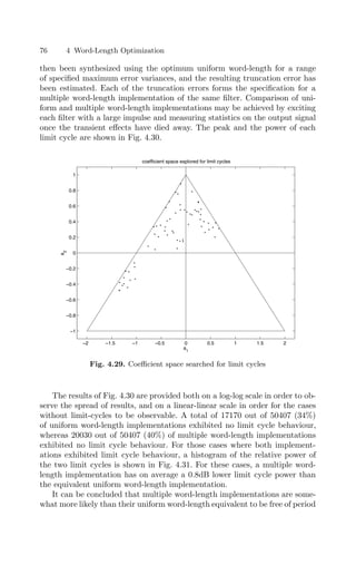
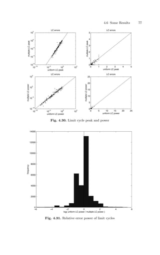
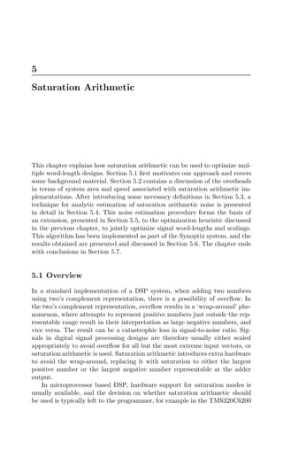
![80 5 Saturation Arithmetic
DSP [TI] or the MMX extensions to the Pentium [PW96]. For direct im-
plementation in hardware, the choice of whether or not to use saturation
arithmetic is particularly important due to the associated cost of the extra
saturation logic in area and delay.
For LTI systems, if 1 scaling is used, as in Chapter 4, overflow is not an
issue and therefore standard arithmetic is to be preferred. In some cases 1
scaling can be overly pessimistic, catering for situations that are extremely
rarely encountered with practical input signals. Overly pessimistic signal scal-
ing can lead to a number of most significant bits (MSBs) in a datapath being
left unused. This is true particularly in the case of filters with long impulse
responses. Under these circumstances an alternative scaling scheme could be
used to reduce the datapath width and therefore save implementation area
and power consumption, however overflow becomes a distinct possibility. It
is in these situations that saturation arithmetic becomes a useful implement-
ation scheme, to limit the impact of these overflows on the overall system
signal-to-noise ratio.
A reasonable design approach, when creating a saturation arithmetic im-
plementation of a DSP system, is to determine signal scaling through simu-
lation. Input vectors are supplied to the system, and the peak value reached
by each internal signal is recorded. Signals are then scaled to ensure that the
full dynamic range afforded by the signal representation would be used un-
der excitation with the given input vectors. In contrast, this chapter presents
an optimization technique suitable for LTI systems, based on analytic noise
models.
5.2 Saturation Arithmetic Overheads
Saturation arithmetic is not a cost-free design methodology. The implementa-
tion of a saturation arithmetic component has some area and delay overheads
associated with it, when compared to the equivalent non-saturation compon-
ent.
Traditionally, saturation arithmetic has been associated with the addition
operator [Mit98]. However there are also circumstances where saturation may
be appropriate following a multiplication. Consider for example a (7, 0) signal
which uses its full dynamic range, and therefore has a peak of ±(1 − 2−7
).
We may multiply this signal by a (7, 1) coefficient with value 1 + 2−6
. The
resulting signal will therefore have a peak of ±(1+2−6
−2−7
−2−13
), although
the (14, 1) format for this signal could represent peaks of up to ±(21
− 2−13
),
approximately double the range. It is intuitive, therefore, that a saturation
by one bit after the multiplication would rarely saturate to its peak values,
and choosing a (13, 0) representation for the result rather than (14, 1) may
result in a more efficient implementation at only a small cost in saturation
error. The technique described in this chapter generalizes the approach, to](https://image.slidesharecdn.com/optimizationandpreparationprocesses-240125021124-f0b0fb42/85/optimization-and-preparation-processes-pdf-93-320.jpg)
![5.2 Saturation Arithmetic Overheads 81
allow saturators to be inserted after any operator: primary input, addition,
delay or constant coefficient multiplication.
Another standard approach to saturation arithmetic is to saturate only
a single most significant bit (MSB). A standard saturation would therefore
convert an (n, p) representation into an (n − 1, p − 1) representation. This
design approach derives from having a single n-bit accumulator. The approach
taken in this chapter does not constrain the design space in this way, and
indeed can saturate different signals to different degrees, in order to trade off
implementation area with implementation error.
The key component introduced and studied in this chapter is therefore a
saturator, as defined in Definition 5.1 and illustrated in Fig. 5.1 for a k-bit
saturator applied to an (n + 1)-bit two’s complement signal. The symbols
used follow IEEE standard [IEE86]: specifically ‘=1’ refers to an ‘or’ gate,
‘G1’ to the common select line of the two-input multiplexers, and inversion is
indicated by a triangle. From this architecture, a simple area cost model can be
deduced for the saturator: A(n, k) = c1k+c2n, where c1 and c2 are empirically
derived constants which may vary with target architecture. The cost function
used in Section 4.2 must therefore be modified to incorporate this additional
cost. Of course, the output of every operator need not be saturated: following
the notation of Section 4.1.1, saturation is never needed if pj = p
j for a signal
j, because the full output range is required. In addition for an LTI system, if
there is no signal j such that pj is less than the value suggested by 1 scaling,
then the system is free from overflow and the saturation area model need not
be used, even if there is a signal j with pj p
j.
Definition 5.1. A saturator is a circuit component, as illustrated in Fig. 5.1,
for converting from format (n, p) to format (n − k, p − k). The parameter k is
referred to as the degree of the k-bit saturator.
Another difference to the area model used in Chapter 4, is that the pre-
viously cost-free computation nodes inport and fork may now have a cost
associated with them due to any saturation nonlinearities at their outputs.
fork is of particular interest, since for a minimal area implementation, a
fork node should be implemented as a cascade of saturators as shown in
Fig. 5.2.
In addition to the area overhead of saturation arithmetic, there will also be
some delay penalty associated with the saturator. Fig. 5.3 illustrates how the
placed and routed propagation delay across a saturation arithmetic constant
coefficient multiplier varies with input word-length for a fixed coefficient value
and for 1-bit saturation. This figure shows a very significant timing overhead
for saturation arithmetic, up to 73%.
To summarize, saturation arithmetic provides advantages in terms of al-
lowing controlled overflows that may not dramatically affect the output signal-
to-noise ratio. However these advantages are provided at the cost of a some-
what larger and slower circuit compared to standard two’s complement arith-
metic for the same binary point locations and word-lengths. In a given imple-](https://image.slidesharecdn.com/optimizationandpreparationprocesses-240125021124-f0b0fb42/85/optimization-and-preparation-processes-pdf-94-320.jpg)
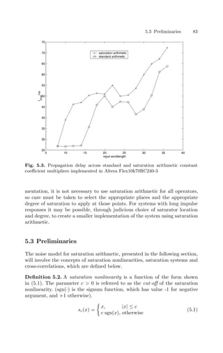
![84 5 Saturation Arithmetic
A saturation nonlinearity can be considered as a generalized model for a
two’s complement saturator. The nonlinearity is more general as the cut-off
used to model a two’s complement saturator will be an integral power of two,
however there is no such restriction on saturation nonlinearity cut-off.
Definition 5.3. A saturation system is a system constructed from a Linear
Time Invariant system by introducing at least one saturation nonlinearity at
an output of an operation. At least one of these nonlinearities must have a
cut-off less than the 1 peak value at that output. The Linear Time Invariant
system from which the saturation system is constructed is referred to as the
underlying LTI system.
The formal representation of a saturation system is as a saturation com-
putation graph GS(V, S, C), as defined below.
Definition 5.4. A saturation computation graph GS(V, S, C) is an annotated
form of a computation graph G(V, S).
The set C takes the form C = {(j1, c1), (j2, c2), . . . , (jp, cp)}, where ji ∈ S
and ci ∈ (0, ∞). C models the position ji and cut-off ci of each saturation
nonlinearity 1 ≤ i ≤ p in the saturation system.
Note that in some graphical representations of a saturation system, the sat-
uration nonlinearities will be explicitly shown. These are not to be considered
nodes in the saturation computation graph GS(V, S, C), but are rather im-
plicit in the choice of annotation C. Similarly the formal representation of a
fixed-point realization of a saturation system is simply an annotated compu-
tation graph G
(V, S, A) (Definition 2.5). The saturator locations are implicit
in the choice of annotation A.
Definition 5.5. The cross-correlation function rxy[τ] between two statistic-
ally stationary random processes x and y is defined to be rxy[τ] = E{x[t]y[t−
τ]}.
5.4 Noise Model
A fixed-point approximate realization of a saturation system is a nonlinear dy-
namical system containing two types of nonlinearities: saturations and trunca-
tions. Saturations are large-scale nonlinearities affecting the most significant
bits of a word, whereas truncations are small-scale nonlinearities affecting a
few of the least significant bits of a word. There is therefore good reason to
consider the two effects separately, and also good reason to assume that these
errors are approximately uncorrelated since correlation between high-order
and low-order bit patterns is unlikely. The exception is if the saturation non-
linearities are so extreme (have such low cut-offs compared to the dynamic
range of the saturated signal) that the probability density function used in](https://image.slidesharecdn.com/optimizationandpreparationprocesses-240125021124-f0b0fb42/85/optimization-and-preparation-processes-pdf-97-320.jpg)
![86 5 Saturation Arithmetic
2
x[t] y[t]
z
-1
+
(a) initial ill-conditioned
structure
-3
p=-1
p=2
p’=1
p=0
p’=0
p=0
p’=0
2
x[t] y[t]
z
-1
+ -2
p=-1
p=1
p’=0
p=-1
p’=-1
p=-1
p’=-1
2
x[t] y[t]
z
-1
+ -2
p=-1
p=0
p’=0
p=-2
p’=-2
p=-2
p’=-2
(b) intermediate ill-conditioned
structure
(c) final well-conditioned
structure
Fig. 5.4. An example of scaling conditioning
zero-mean Gaussian variable also forms another zero-mean Gaussian variable.
It therefore follows that all internal signals in an LTI system driven by zero-
mean Gaussian inputs will themselves be zero-mean Gaussian, since all signals
can be expressed as a weighted sum of present and past inputs. The Gaussian
assumption is also useful because the joint pdf fXY (x, y) of two zero-mean
Gaussian variables X and Y is completely known from their respective vari-
ances and correlation coefficient, defined as γ = E{XY }/ E{X2}E{Y 2}.
In reality, however, inputs may follow a large variety of distributions which
will cause the intermediate signals in the modelled system to deviate to some
extent from their idealized Gaussian form. The assumption is that such a de-
viation will be small enough for practical cases and for the purposes to which
this model will be put. Often the largest deviation from the Gaussian model
is likely to be at the primary inputs to the system, since the internal nodes
are formed by a weighted sum of present and past input values. In the most
extreme example, where the LTI system under investigation approaches a nor-
malized integrator (transfer function H(z) = lim
n→∞
n−1
(1 − z−n
)/(1 − z−1
) )
and the input is made up of a stream of independent identically distributed
(iid) random variables, the Gaussian approximation will clearly hold no mat-
ter what the input distribution, by the central limit theorem. In more general
cases there are an abundance of extensions to the central limit theorem for
specific relaxations of the constraints on independence and identical distribu-
tion [Chu74]. While there is no general theoretical result for all cases, it is
reasonable to assume that bell-shaped distributions are common in practice,
and evidence to support the assumption is available in Section 5.4.6, where
modelling results are compared to simulations of ‘real-world’ speech input
data.](https://image.slidesharecdn.com/optimizationandpreparationprocesses-240125021124-f0b0fb42/85/optimization-and-preparation-processes-pdf-99-320.jpg)
![5.4 Noise Model 87
The introduction of saturation nonlinearities into the system significantly
complicates the picture. The saturated Gaussian distribution, as defined below
and illustrated in Fig. 5.5, is used to model the pdf at each internal signal
within a saturation system.
Definition 5.6. A random variable X follows a saturated Gaussian distribu-
tion with parameters (σ, c) where σ ≥ 0 and c ≥ 0 iff its probability density
function fX(x) has the form given in (5.2). The Gaussian distribution with
mean 0 and standard deviation σ is referred to as the underlying distribution.
fX(x) =
Q(c/σ) (δ(x − c) + δ(x + c)) + 1
σ
√
2π
exp(− x2
2σ2 ), if |x| ≤ c
0, otherwise
(5.2)
Here δ(·) is the Dirac delta function [Gar90] and Q(·) represents the ‘upper
tail’ function of the standard Gaussian distribution.
−2 −1.5 −1 −0.5 0 0.5 1 1.5 2
−0.1
0
0.1
0.2
0.3
0.4
0.5
x
f
X
(x)
Fig. 5.5. The saturated Gaussian distribution with parameters (σ = 1, c = 1.5)
Since the pdf is an even function, all odd moments of the probability
distribution vanish to zero. Expressions are provided below for the second and
fourth moment of the saturated Gaussian, which will be used for modelling
purposes.](https://image.slidesharecdn.com/optimizationandpreparationprocesses-240125021124-f0b0fb42/85/optimization-and-preparation-processes-pdf-100-320.jpg)
![88 5 Saturation Arithmetic
The second moment (variance) of a saturated Gaussian distribution can
be calculated though (5.3).
µ2 = σ2
− 2
Q(c/σ)(σ2
− c2
) +
cσ
√
2π
exp(−
c2
2σ2
)
(5.3)
The fourth moment (related to Kurtosis) of a saturated Gaussian distri-
bution can be calculated through (5.4).
µ4 = 3σ4
− 2
Q(c/σ)(3σ4
− c4
) +
1
√
2π
cσ(c2
+ 3σ2
) exp(−
c2
2σ2
)
(5.4)
Multiplication of a saturated Gaussian random variable of parameters
(σ, c) by a constant factor k results in a random variable with saturated
Gaussian distribution of parameters (kσ, kc). Clearly the multiple outputs of
a branching node whose input has parameters (σ, c) will all have the same
parameters (σ, c), and the output of a delay node will behave in a similar
manner.
Let X be one such post-multiplication, post-branching, or post-delay sat-
urated Gaussian signal. This signal may then itself be saturated by a nonlin-
earity with cut-off c̄. The variance of the associated error e injected at the
point of saturation can be calculated as in (5.5), where fX̂(x) is the pdf of
the underlying Gaussian distribution of X.
E{e2
} =
2
c
c̄ (c̄ − x)2
fX̂(x)dx + (c̄ − c)2
Q(c/σ), c̄ c
0, otherwise
=
2(c − c̄)2
Q(c/σ) + 2(c̄2
+ σ2
) [Q(c̄/σ) − Q(c/σ)] +
2σ
√
2π
(2c̄ − c) exp(− c2
2σ2 ) − c̄ exp(− c̄2
2σ2 )
, c̄ c
0, otherwise
(5.5)
For addition the situation is more complex, and is addressed in the follow-
ing section.
5.4.3 Addition of Saturated Gaussians
While the addition of two Gaussian random variables follows a Gaussian dis-
tribution, it is not true that the addition of two saturated Gaussian random
variables follows a saturated Gaussian distribution. In fact, the distribution
formed by their addition may follow a number of forms depending on the
correlation between the two inputs to the addition, and their respective ‘c’
parameters. Fig. 5.6 illustrates an addition followed by a saturation nonlin-
earity.](https://image.slidesharecdn.com/optimizationandpreparationprocesses-240125021124-f0b0fb42/85/optimization-and-preparation-processes-pdf-101-320.jpg)
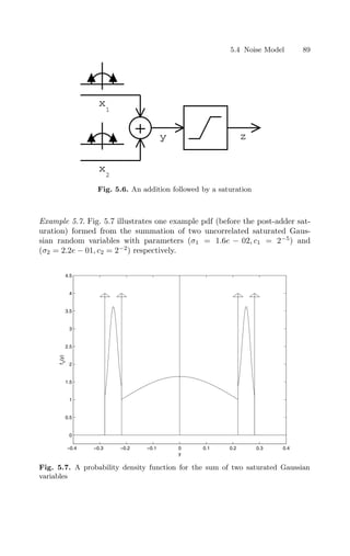
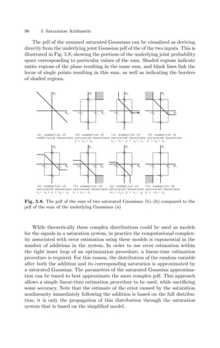
![5.4 Noise Model 91
The ‘tuning’ of model parameters can be performed through matching all
statistical moments of the two distributions, up to and including the fifth
moment. The procedure is as follows: firstly the ‘true’ second and fourth mo-
ment of the saturated sum are calculated, and secondly the model parameters
(σm, cm) are chosen to match these moments. In order to calculate the ‘true’
moments and correlation coefficients for each addition, the transfer functions
from each primary input to each adder input must be known.
Example 5.8. Since saturation arithmetic is particularly useful for IIR filters,
we consider here a second order Direct Form II transposed IIR section, typic-
ally used as a building block for larger order IIR filters [Mit98]. Such an IIR
section is illustrated in Fig. 3.2, reproduced in Fig. 5.9 for convenience where
each addition has been labelled A1 to A4.
b b
z
-1
+ + + z
-1
+
b
-a -a
0
1
1
2
2
A4
A3
A2
A1
x
y
Fig. 5.9. A second order IIR section
The covariance calculations at each adder are provided in (5.6) for com-
pleteness. In order to be able to calculate the correlations between inputs to
adders for a second order section, we therefore require rxy[τ] for τ = −1, 0, 1, 2,
rxx[τ] for τ = 1, 2 and ryy[τ] for τ = 1. These values can be calculated knowing
rxx and the transfer functions to each adder input in the system.
A4: E{−b2x[n]a2y[n]} = −b2a2rxy[0]
A3: E{b1x[n](b2x[n − 1] − a2y[n − 1])} = b1b2rxx[1] − b1a2rxy[1]
A2: E{−a1y[n](b1x[n] + b2x[n − 1] − a2y[n − 1])} =
−a1b1rxy[0] − a1b2rxy[−1] + a1a2ryy[1]
A1: E{b0x[n](−a1y[n − 1] + b1x[n − 1] + b2x[n − 2] − a2y[n − 2])} =
−a1b0rxy[1] + b0b1rxx[1] + b0b2rxx[2] − b0a2rxy[2]
(5.6)
It is important to note that these calculations do not depend in any way
on the actual cut-off values for the saturation nonlinearities since they are](https://image.slidesharecdn.com/optimizationandpreparationprocesses-240125021124-f0b0fb42/85/optimization-and-preparation-processes-pdf-104-320.jpg)
![92 5 Saturation Arithmetic
calculated from the underlying LTI system. This means that correlation coef-
ficients need only be calculated once for a given system, before entering the
optimization loop.
The next phase in the algorithm is to match the calculated moments to a
saturated Gaussian model. The matching is a relatively computationally inex-
pensive operation, because there already exist good intuitive starting guesses
for the two parameters, namely σ
(0)
m = σ2
1 + σ2
2 + 2γσ1σ2, and c
(0)
m = c̄,
where γ is the correlation coefficient of the underlying Gaussian inputs and
c̄ is the cut-off of the post-adder saturation nonlinearity. Since µ2 and µ4 for
the model, (5.3) and (5.4) respectively, are differentiable it is straightforward
to use a 2-dimensional extension of the Newton-Raphson method [OR70] to
select the model parameters. The Jacobian is shown in (5.7).
J =
∂µ2
∂σ
∂µ2
∂c
∂µ4
∂σ
∂µ4
∂c
!
= 2
σ(1 − 2Q(c/σ)) − 2c
√
2π
exp(− c2
2σ2 ) 2cQ(c/σ)
6σ3
(1 − 2Q(c/σ)) − c
√
2π
exp(− c2
2σ2 ) 4c3
Q(c/σ)
(5.7)
Since a saturation system is a nonlinear dynamical system, estimation
of γ for each addition is based on the equivalent correlation coefficient in the
underlying LTI system. This is a reasonable assumption when the overall level
of saturation in the system is small, which will generally be the case unless
extremely low SNR is allowable.
A standard iterative update scheme is used, as shown in (5.8).
σ
(n+1)
m
c
(n+1)
m
=
σ
(n)
m
c
(n)
m
− J−1
µ
(n)
2
µ
(n)
4
(5.8)
5.4.4 Error Propagation
As with the truncation error estimation described in Section 4.1.2, in order
to propagate the saturation error to the outputs of the system, the saturation
nonlinearities are linearized as shown for an example in Fig. 5.10. This allows
the use of linear system theory to predict the effect of this saturation error
on the output signal-to-noise ratio. However unlike the truncation case, it
cannot be assumed that the saturation errors injected at various points within
the structure are uncorrelated. Recall that for the truncation noise model,
this approximation is reasonably valid because it is the least significant bits
that are being quantized, which have little relationship to other sets of least
significant bits being truncated at other points. The same cannot be said for
the saturation nonlinearities. Taking the example in Fig. 5.10, it is clear that
when e1[t] 0, there will be a greater probability of e2[t] being negative than
if e1[t] ≥ 0 because there will be a greater probability of the post-adder signal
value being large and positive if the primary input is large and positive. In
addition, the white assumption on each individual error input is not valid for
saturation errors, since the spectrum of the error sequence will clearly depend](https://image.slidesharecdn.com/optimizationandpreparationprocesses-240125021124-f0b0fb42/85/optimization-and-preparation-processes-pdf-105-320.jpg)
![5.4 Noise Model 93
heavily on the (possibly coloured) spectrum of the input sequence. These two
dimensions of dependence, between pairs of error inputs and over time, require
a more sophisticated error estimation model.
0.1
+
x[t] y[t]
z
-1
0.1
x[t] y[t]
z
-1
+
+ +
e[t]
1 e[t]
2
(a) a saturation system
(b) the corresponding linearization
Fig. 5.10. Linearization of the saturation nonlinearities
Estimating the cross-correlation function between saturation inputs is pos-
sible but computationally intensive. Although in general there is no solution
to this problem in linear time, a bound can certainly be placed on the error
power at the system outputs, and this bound can be calculated in linear time.
Claim. In a saturation system let there be a total of p saturation nonlinear-
ities, with corresponding linearized error inputs e1, . . . , ep of standard devi-
ations σe1 , . . . , σep . Let us concentrate on a single primary output with error y,
and let Hi(z) denote the transfer function from error input ei to this output.
Then (5.9) holds.
E{y2
[t]} ≤
p
i=1
σei 1{Hi(z)}
2
(5.9)
Proof:
The value of the error y at time index t (at any specific output) is then given
by the convolution in (5.10). Here bi represents the impulse response from
error input i to the output in question.
y[t] =
p
i=1
∞
k=0
ei[t − k]bi[k] (5.10)](https://image.slidesharecdn.com/optimizationandpreparationprocesses-240125021124-f0b0fb42/85/optimization-and-preparation-processes-pdf-106-320.jpg)
![94 5 Saturation Arithmetic
Assuming statistically stationary input signals, we obtain (5.11) for the
general saturation-induced error power at the output. Here rei1 ei2
is the cross-
correlation function rei1 ei2
[τ] = E{ei1 [t]ei2 [t − τ]}.
E{y2
[t]} =
p
i1=1
p
i2=1
∞
k1=0
∞
k2=0
bi1 [k1]bi2 [k2]rei1 ei2
[k2 − k1] (5.11)
The Cauchy-Schwartz inequality (5.12) [Gar90] may be invoked, allow-
ing (5.11) to be separated, as in (5.13). Here σei represents the standard
deviation of error input ei and Hi(z) is the transfer function from that input
to the output in question.
E2
{XY } ≤ E{X2
}E{Y 2
}
for zero-mean random variables X and Y
(5.12)
E{y2
[t]} ≤
p
i1=1
p
i2=1
∞
k1=0
∞
k2=0
|bi1 [k1]bi2 [k2]|σei1
σei2
≤
p
i=1
σei 1{Hi(z)}
2 (5.13)
Of course such a bound may be more or less close to the empirical error
power. The true measure of usefulness for this bound in real applications, is
that the circuits synthesized using this measure of error are at least of com-
parable area to those synthesized using traditional simulation-based average
case scaling, preferably smaller. This measure will be tested in Section 5.6.
5.4.5 Reducing Bound Slackness
There are certain transformations which may be performed on the graph rep-
resentation of a saturation system without affecting the global system beha-
viour. A saturation nonlinearity may be moved through a constant coefficient
multiplication, a move accompanied by a corresponding scaling in the satur-
ation cut-off parameter (Fig. 5.11(a)). In addition, two consecutive nonlin-
earities can be merged (Fig. 5.11(b)), and multiple nonlinearities following a
branching node can be reconfigured (Fig. 5.11(c)). Although these transforma-
tions do not result in different system behaviour from an external perspective,
the estimated saturation error resulting from the procedure described above
can differ, due to different slackness in the Cauchy-Schwartz derived upper
bound. It is useful to minimize this slackness. Note that the transformation
in Fig. 5.11(c) has been used in Section 5.2 to minimize the implementation
cost of a fork node. However the two applications of this transformation](https://image.slidesharecdn.com/optimizationandpreparationprocesses-240125021124-f0b0fb42/85/optimization-and-preparation-processes-pdf-107-320.jpg)
![5.4 Noise Model 95
K
c
c
K K
(a)
(c)
c
c
z
-1
z
-1 c1 c2
(b)
min(c ,c )
1 2
c1 c2 cn
...
c c
1 2
...
cn
for c = c = ... = c
1 2 n
Fig. 5.11. Useful saturation transformations
are entirely separate: applying the transformation for saturation error mod-
elling in no way suggests altering the physical realization of the saturation
nonlinearity.
Example 5.9. Applying these transformations to the second order section
shown in Fig. 5.12(a) results in the improved saturation system in Fig. 5.12(b);
W1 and W2 are wiring constructs where the outputs are a permuted version
of the inputs, and S1 and S2 are saturation constructs with possible forms
illustrated in Figs. 5.12(c) and (d) respectively. Applying the saturation noise
model to this construction can result in a tighter Cauchy-Schwartz bound.
Claim. For the transformation shown in Fig. 5.11(b), it is always desirable to
merge the two nonlinearities.
Proof:
Let the linearized error inputs at the saturation nonlinearities with cut-offs c1
and c2 be e1[t] and e2[t] of variance σe1 and σe2 , respectively. Similarly, let the
error input at the saturation nonlinearity with cut-off min(c1, c2) be e[t] of
variance σe. Since there are no branches between nonlinearities, (5.13) will not
be increased by merging iff the error standard deviations obey σe1 +σe2 ≥ σe.
However it is clear that e[t] = e1[t] + e2[t] and therefore application of (5.12)
reveals that this is indeed the case since σ2
e = σ2
e1
+ σ2
e2
+ 2E{e1[t]e2[t]} and
σe1 + σe2 ≥ σe ⇔ σ2
e1
+ σ2
e2
+ 2σe1 σe2 ≥ σ2
e.
The transformation shown in Fig. 5.11(c) will not always improve the error
bound, since the 1 scaling from saturation error with cut-off ci, 1 ≤ i n, is
different in the two cases. Although the error injected due to the saturations
with cut-offs cj, 2 ≤ j ≤ n may be reduced, whether this is offset by the change
in scaling is dependent on the system transfer functions. For a general n-way](https://image.slidesharecdn.com/optimizationandpreparationprocesses-240125021124-f0b0fb42/85/optimization-and-preparation-processes-pdf-108-320.jpg)
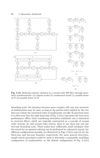
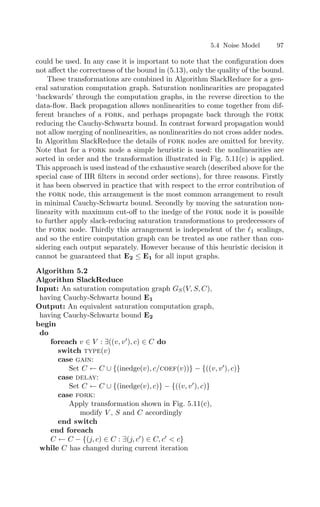
![98 5 Saturation Arithmetic
end
5.4.6 Error estimation results
This section presents some results from using the error model discussed thus
far to predict saturation error variance. Approximately 6000 IIR filters have
been generated, each filter having between second and tenth order. The feed-
back coefficients are generated by randomly choosing complex conjugate pole
locations in the range 0 |z| 0.998 and 0 arg(z) π (uniformly distrib-
uted), and the feed-forward coefficients are generated by randomly distribut-
ing them between 0 and 1 (uniformly distributed). 1 scaling is then applied
to each filter, and the binary point locations are decided by choosing either
those through 1 scaling or one or two bits beneath this value, each location
independently of the other. Probabilities are skewed such that there is a mean
of two saturation nonlinearities in each section, in order to agree with typical
synthesized circuits. The choice of saturator degree is decided with uniformly
distributed probability and independently of all other saturation locations.
The predicted error variance is then compared to the observed variance ar-
rived at through a bit-true simulation of the system. Two types of input data
are used: independent identically distributed Gaussian input samples, and real
speech data [FRE93].
Fig. 5.13 presents several plots of the error bound, derived through the
technique presented in this chapter, against a simulation run. Fig. 5.14
presents the data as a histogram of over-estimation ratios, and also illus-
trates how this histogram changes with the order of the filter modelled for the
iid case. It is clear that for the large majority of designs the Cauchy-Schwartz
bound provides a value between 0dB and 50dB greater than the simulated
result. Although both the slackness of the bound derived, and the mismatch
between the saturated Gaussian model and post-addition pdf grow with the
order of the filter, it is not a rapid growth. From fourth to tenth order the
bulk of overestimation ratios lie in the same range, with little change in the
spread of the distribution. Recall that the error estimation is for average-case
behaviour, and so the bound is on the expected error variance, not the er-
ror variance for each specific case. In addition the bound is only exact if the
standard deviations of the injected errors are known exactly, whereas in real-
ity they are estimated through modelling signals as saturated Gaussians, as
discussed previously. There is some mismatch between the input probability
density function and the Gaussian assumption for speech, leading to margin-
ally worse performance in the speech case (speech pdf falls off as exp(−λ1|x|)
rather than the Gaussian exp(−λ2x2
) [P50]).
Whether the noise model is sufficient for optimization purposes can only
be measured by the quality of the circuits produced by the optimization pro-
cedure, which will be discussed in the following section.](https://image.slidesharecdn.com/optimizationandpreparationprocesses-240125021124-f0b0fb42/85/optimization-and-preparation-processes-pdf-111-320.jpg)
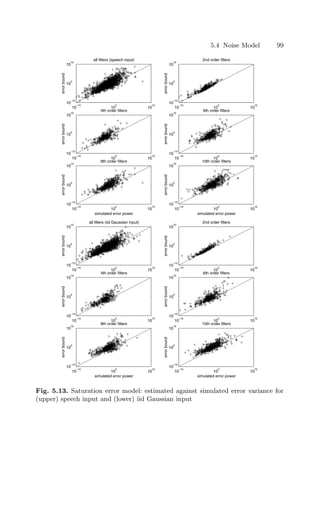
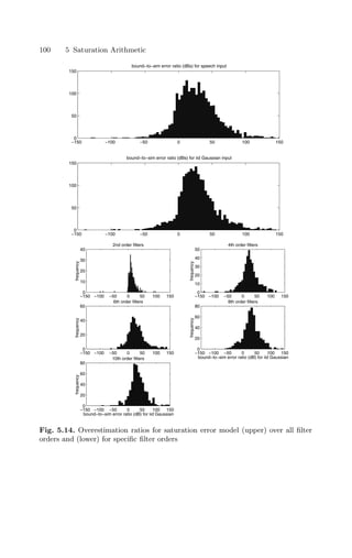
![5.5 Combined Optimization 101
5.5 Combined Optimization
The method presented in Section 5.4 can be used to form an estimate
EG(n, p, R) of the error variances incurred through the implementation of
computation graph G with word-lengths n, binary point locations p, and in-
put correlation matrix R[τ] = E{x[t]x[t − τ]T
}, where x is the vector of sys-
tem primary inputs. This estimate may then be compared to the user-specified
bounds E on error variance at each output.
Since both the scaling and the word-length of each signal can have an
impact on system error and area, the problem of finding a suitable annotation
for the computation graph must now be treated as the combined optimization
problem formulated below c.f. the Word-length Optimization Problem from
Chapter 4.
Problem 5.10 (Combined Word-length and Scaling Optimization).
Given a computation graph G(V, S) and correlation matrix R, the combined
word-length and scaling optimization problem may be defined as to
select (n, p) such that AG(n, p) is minimized subject to (5.14).
n ∈ N|S|
p ∈ Z|S|
EG(n, p, R) ≤ E
(5.14)
To solve this optimization problem, it is necessary to modify Algorithm
Word-LengthFalling from Section 4.4 to incorporate the optimization of bin-
ary point locations. This is performed by Algorithm CombOptAlg, where 1
represents a vector of ones of appropriate size, and k is the scaling factor as
described in Section 4.4. Bj is a lower bound on the binary point location
of signal j. Typically Bj is set to be a fixed, but reasonably large, number
of bits beneath the binary point location implied by 1 scaling. Although Bj
is rarely reached in practical designs with realistic error constraints, these
bounds are required to theoretically ensure termination of Algorithm Comb-
OptAlg. Reaching pj = Bj is considered equivalent to pj ∼ −∞. The inter-
pretation of this value is that it is unnecessary to calculate signal j in order
to satisfy the error constraints, and so the entire cone of logic creating signal
j may be optimized away.
Unlike the error estimation used in Algorithm Word-LengthFalling, the
error estimation subroutine used in Algorithm CombOptAlg contains some
computationally expensive calculations, namely the post-adder saturation er-
ror and pdf estimation, which involves numerical integration and series ap-
proximations [AS70]. However the calls to adder saturation error estimation
routines in the above algorithm exhibit a high degree of temporal locality. It
is highly probable that a given pj will not change from one iteration to the
next, and therefore the same error estimations are often required. Rather than
re-calculate these each time, new error estimates for a given adder are only](https://image.slidesharecdn.com/optimizationandpreparationprocesses-240125021124-f0b0fb42/85/optimization-and-preparation-processes-pdf-114-320.jpg)

![Algorithm 5.3
Algorithm CombinedOptHeur
Input: A Computation Graph G(V, S)
input correlation matrix R
Output: An Optimized Annotated Computation
Graph G
(V, S, A), (A = (n, p))
begin
Calculate the variance of each signal and the correlation coefficient between
inputs to adders, to be used in all calls to the error estimation subroutine
Set p ← 1 scaling vector (as described in Section 3.1.1)
Determine u, the minimum uniform word-length satisfying EG(u · 1, p, R) ≤ E
Set n ← ku · 1
do
Condition the graph G
(V, S, A)
Set currentcost ← AG(n, p)
foreach signal j ∈ S do
Set bestmin ← currentcost
Determine w ∈ {2, ..., nj}, if such a w exists, such that
EG([n1 . . . nj−1 w nj+1 . . . n|S|]T
, p, R) ≤ E and
EG([n1 . . . nj−1 (w − 1) nj+1 . . . n|S|]T
, p, R) E
If such a w exists, set minval ← AG([n1 . . . nj−1 w nj+1 . . . n|S|]T
, p)
If no such w exists, set minval ← AG([n1 . . . nj−1 1 nj+1 . . . n|S|]T
, p)
if minval bestmin do
Set bestsig ← j, bestmin ← minval, vartype ←word-length
end if
Determine x ∈ {Bj + 1, ..., pj − 1, pj}, if such an x exists, such that
EG(n, [p1 . . . pj−1 x pj+1 . . . p|S|]T
, R) ≤ E and
EG(n, [p1 . . . pj−1 (x − 1) pj+1 . . . p|S|]T
, R) E
If such an x exists, set minval ← AG(n, [p1 . . . pj−1 x pj+1 . . . p|S|]T
)
If no such x exists, set minval ← AG(n, [p1 . . . pj−1 Bj pj+1 . . . p|S|]T
)
if minval bestmin do
Set bestsig ← j, bestmin ← minval, vartype ←scaling
end if
end foreach
if bestmin currentcost
if vartype = word-length
nbestsig ← nbestsig − 1
else
pbestsig ← pbestsig − 1
while bestmin currentcost
end
5.5 Combined Optimization 103](https://image.slidesharecdn.com/optimizationandpreparationprocesses-240125021124-f0b0fb42/85/optimization-and-preparation-processes-pdf-116-320.jpg)
![104 5 Saturation Arithmetic
5.6 Results and Discussion
Algorithm CompOptAlg has been implemented in MATLAB [MAT] in order
to leverage its numerical integration routines, at the cost of increased exe-
cution time over an extension to the C implementation used in Chapter 4.
However all execution runs discussed in this section are completed within
10 minutes on a Pentium III 450MHz, compared to 4 minutes for a Matlab
implementation of Algorithm Word-LengthFalling and 10 seconds for calcu-
lation of the optimum uniform word-length. In addition, the execution time
of Algorithm CombOptAlg will grow at the same rate as that of Algorithm
Word-LengthFalling.
To illustrate the applicability of saturation arithmetic optimization to dif-
ferent types of design, two 4th order IIR filers are generated. One is a narrow
bandpass elliptic filter, and one is a lowpass elliptic filter. Both filters are to
be driven with a speech input [FRE93]. Clearly the narrow bandpass filter
will have very high theoretical peak values at internal signals, as would be
determined by 1 scaling. However an input signal that would cause internal
signals to reach these peaks is unlikely to be present in a speech signal, which
contains a wide range of frequency components. Thus the ratio between 1
peak value at any signal and the peak value reached during a simulation run
is likely to be relatively large. In contrast the equivalent ratios in the lowpass
filter are likely to be much more modest.
Fig. 5.15 shows an execution trace of Algorithm CombOptAlg executing on
the bandpass filter, illustrating the change in system area and error variance
as the algorithm refines the solution. Two plots are superimposed in the error
variance trace: these are the error due to truncation alone, and the overall
error. It is clear that until iteration 42, the contribution of saturation to the
overall error is negligible. At this iteration the decision is made to reduce a
binary point location of one of the signals, resulting in a significant saturation
error. However by the end of the optimization run it is clear that the truncation
error yet again dominates the saturation error.
5.6.1 Area Results
The standard approach of using simulation to determine signal scaling aims
to avoid overflow for the specific input sequences provided, though not ne-
cessarily for all input sequences. The scaling of each signal through the use
of simulation, and hence the area of a simulation-scaled system, therefore de-
pends on the length of input sequence used for simulation. The longer the
input sequence, the more the ‘tails’ of the pdf of an internal signal are likely
to be encountered. Simulating the system on a short input sequence may res-
ult in a smaller area at the cost of a larger saturation error on unencountered
input sequences, when compared to lengthy simulation runs.
In contrast, Algorithm CombOptAlg tolerates overflow errors if these er-
rors help to achieve a small implementation cost, and is able to estimate the](https://image.slidesharecdn.com/optimizationandpreparationprocesses-240125021124-f0b0fb42/85/optimization-and-preparation-processes-pdf-117-320.jpg)
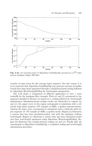
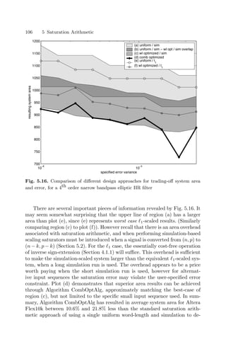
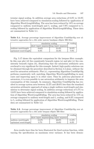
![108 5 Saturation Arithmetic
10
−8
10
−7
550
600
650
700
750
800
specified error variance
resulting
system
area
(a) uniform / sim
(b) wl optimized / sim
(d) comb optimized
(e) uniform / l
1
(f) wl optimized / l1
Fig. 5.17. Comparison of different design approaches for trading-off system area
and error, for a 4th order lowpass elliptic IIR filter
strated that significant area reductions can be achieved for the narrow band-
pass filter example. Fig. 5.18 illustrates how the area consumption of second
order autoregressive filters varies with the location of their complex conjugate
pole on the z-plane, for fixed error specification. Compared to 1 scaling, area
savings have been achieved using the techniques developed in this chapter for
systems with poles with magnitude greater than approximately 0.9.
5.6.2 Clock frequency results
As noted in Section 5.2, there are also significant timing overheads associ-
ated with the use of saturation arithmetic. While Algorithm CombOptAlg
does not explicitly consider circuit speed, it is instructive to place the points
on Fig. 5.16 on a speed / area design-space diagram. This is shown in
Fig. 5.19, where the short simulation run results are used for representation
of simulation-scaled systems. There are ten graphs, corresponding to the ten
error variance specifications in Fig. 5.16. Speed estimates are obtained from
Altera MaxPlus II [MAX] on the fully placed and routed design in an Al-
tera Flex10kRC240-3 device. A Pareto-optimal point [DeM94] is a point in](https://image.slidesharecdn.com/optimizationandpreparationprocesses-240125021124-f0b0fb42/85/optimization-and-preparation-processes-pdf-121-320.jpg)
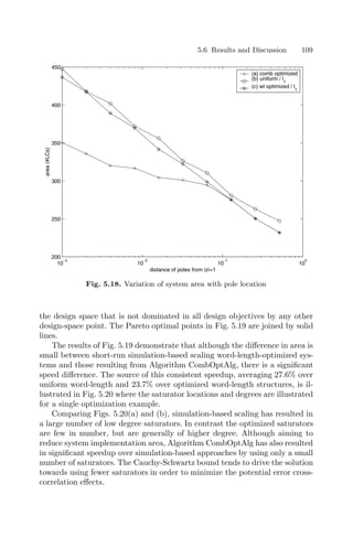
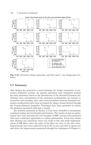
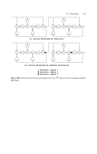

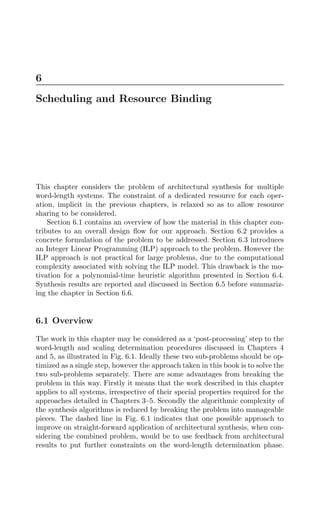
![114 6 Scheduling and Resource Binding
Such constraints could emphasize the sharing of particular resources by redu-
cing the number of free word-length variables in the word-length optimization
problem. However that approach is not addressed in this book. The present
chapter is concerned only with the architectural synthesis block in Fig. 6.1.
architectural
synthesis
algorithm
specification
scaling and
wordlength
optimization
dedicated
resource
architecture
shared
resource
architecture
Fig. 6.1. Overall design flow for general resource binding architectures
6.2 Motivation and Problem Formulation
The synthesis problems addressed in Chapters 4 and 5 both assume that the
architecture resulting from the synthesis process utilizes a dedicated resource
binding. In a dedicated resource binding, each unit sample delay is mapped
to a distinct register, each addition to a distinct adder, and each constant-
coefficient multiplication to a distinct constant-coefficient multiplier. One of
the problems with this approach is that for area-limited architectures such as
FPGAs, very large designs may not be feasible. A solution to this problem is
to share some of the resources between operations, multiplexing the inputs to
these resources over time, and thus allowing a speed / area tradeoff.
The problems of resource allocation (deciding how many resources of a
particular type should be used), resource binding (deciding which operation
is to be executed on which resource), and scheduling (deciding at which clock
period, or ‘time step’, each operation should execute) have all been well stud-
ied [Cam90, McF90, DeM94, Lin97]. However such work in the open literature](https://image.slidesharecdn.com/optimizationandpreparationprocesses-240125021124-f0b0fb42/85/optimization-and-preparation-processes-pdf-127-320.jpg)
![6.2 Motivation and Problem Formulation 115
has invariably considered all operations of a particular type, such as ‘multiply’
or ‘add’, to have identical implementations or at least an identical library of
possible implementations [JPP88, Jai90, IM91, HO93].
There has been very little previous or concurrent research [KS98, CCL00b,
KS01] on architectural synthesis for multiple word-length systems. The mul-
tiple word-length paradigm has a significant impact on the traditional prob-
lems of high-level synthesis, arising from two factors. Firstly, each com-
putational unit of a specific type, for example ‘multiply’, cannot be as-
sumed to have equal cost in a multiple word-length implementation, since
area scales with operator word-length. This issue has been considered by
both [KS98, KS01] and [CCL00b]. Secondly, the choice of word-length for
an operation can impact on the latency of that operation. For instance, lar-
ger bit-parallel multipliers may have longer latency than smaller bit-parallel
multipliers. The existence of multiple word-lengths therefore complicates the
resource binding problem, and also increases the interaction between binding
and scheduling of operations.
Only a single iteration of the specified algorithm, and simplified cost mod-
els are considered in this chapter. Each arithmetic operation v is associated
with a word-length. For an adder, a word-length is a positive integer bA
(v),
representing the bit-width of the core (integer) adder required in order to im-
plement the multiple word-length addition (see Section 4.2). For a multiplier,
a word-length is a pair bM
(v), representing the two input bit-widths of the
core (integer) multiplier required (also see Section 4.2). The elements of the
pair are arranged such that the first element is always greater than or equal
to the second element. Thus for the remainder of this chapter, it is sufficient
to refer to a ‘10-bit addition’ or a ‘23 × 12-bit multiplication’.
These concepts are formalized in the definition of a sequencing graph given
in Definition 6.1.
Definition 6.1. A sequencing graph P(V, D) is a directed acyclic graph
(DAG), representing the data flow during a single iteration of an algorithm.
The set V is in one-to-one correspondence with the set of operations. The
directed edge set D ⊂ V × V is in correspondence with the flow of data from
one operation to another.
As with Definition 2.1, a type function exists for elements of V (6.1).
Each node v ∈ V with type(v) = mult has a word-length tuple bM
(v) =
(pv, qv) ∈ N2
with pv ≥ qv and each node v ∈ V with type(v) = add has a
single word-length bA
(v) ∈ N.
type : V → {add, mult} (6.1)
Example 6.2. A simple sequencing graph is illustrated in Fig. 6.2. The node
set consists of five multiplications and four additions.
The multiple word-length architectural synthesis problem may
now be defined in Problem 6.3. Note that the creation of structural hardware](https://image.slidesharecdn.com/optimizationandpreparationprocesses-240125021124-f0b0fb42/85/optimization-and-preparation-processes-pdf-128-320.jpg)
![116 6 Scheduling and Resource Binding
m
MULT
(18,15)
m
MULT
(19,17)
m
MULT
(33,21)
m
MULT
(22,16)
m
MULT
(40,12)
a
ADD
20
a
ADD
25
a
ADD
22
a
ADD
19
1
2 3
4 5
1
2
3
4
Fig. 6.2. A simple sequencing graph: node labels indicate node name, node type,
and word-length
description language from the resulting information is not considered in this
chapter, as such techniques are well known [PWB92].
Problem 6.3 (MULTIPLE WORD-LENGTH ARCHITECTURAL
SYNTHESIS). Given a sequencing graph P(V, D), and a specified max-
imum latency λ, determine
• a set of resources and their associated word-lengths Y
• a mapping from operation to resource R : V → Y
• a mapping from operation to time-step S : V → N ∪ {0}
such that the area consumed by the set of resources is minimal, all data-
dependencies are preserved, no resource executes more than one operation in
each clock cycle, and the entire sequencing graph completes within λ cycles.
Each resource y ∈ Y has a word-length b(y) ∈ N for an adder and b(y) ∈ N2
for a multiplier resource. For each target architecture, it is necessary to con-
struct an empirically derived function which determines the required number
of clock cycles for each multi-cycle resource word-length r. This construction
has been performed for the Sonic architecture [HSCL00] for word-lengths up
to 64-bits, the results of which are given in (6.2).
L(r) =
(p + q)/8, r = (p, q) ∈ N2
2, r ∈ N
(6.2)](https://image.slidesharecdn.com/optimizationandpreparationprocesses-240125021124-f0b0fb42/85/optimization-and-preparation-processes-pdf-129-320.jpg)
![6.3 Optimum Solutions 117
The cost function used for each resource is given in terms of its word-
length in (6.3), where k ∈ R is a technology-dependent constant representing
the relative cost of adder and multiplier implementations.
cost(r) =
p · q, r = (p, q) ∈ N × N
k · r, r ∈ N
(6.3)
Example 6.4. As a motivational example, consider again the sequencing graph
representing data-dependencies shown in Fig. 6.2. An area-optimal schedule,
binding and word-length selection for this sequencing graph is illustrated in
Fig. 6.3 for the case k = 1 and no operation pipelining. This resource allocation
consists of two adders: one of 25-bits and one of 19-bits, and three multipliers:
one is a 19 × 17-bit multiplier, one a 33 × 17-bit multiplier, and one a 40 × 12-
bit multiplier. The graphical matrix illustrates which resource is being used
by which operation at which time step.
Note that in Fig. 6.3 resources can perform operations up to the word-
length of the resource, even if implementation in a larger resource leads to
a longer latency than a ‘tight-fitting’ resource would require. For example
operation m4 is implemented in a resource of latency 7 cycles, although its
word-length only requires a 22 × 16-bit multiplier which would take only 5
cycles to complete. This ‘stretching’ of operations that are not on the critical
path can conceivably lead to significantly reduced area, by exposing possibil-
ities for resource sharing.
6.3 Optimum Solutions
Integer Linear Programming (ILP) [GN72] has been used in high-level syn-
thesis for some time [HLH91, Ach93, LP93, DeM94, LMD94]. This section
presents an extension to these ILP formulations in order to solve Prob-
lem 6.3 [CCL00c]. Formulation as an ILP is useful from an analytical per-
spective, because it formalizes the problem and its constraints. In addition,
for small problem instances, ILP solvers such as lp solve [Sch97] may be
used to obtain globally optimum solutions to the synthesis problem. These
optimum solutions are valuable references for comparison with heuristic ap-
proaches.
6.3.1 Resources, Instances and Control Steps
Before presenting the ILP formulation of Problem 6.3, it is necessary to define
certain quantities and notations, to be used in the following sections.
The starting point for the ILP approach is a sequencing graph P(V, D) and
a target overall latency constraint λ. The latency constraint corresponds to a
user-specified upper bound on the number of clock cycles which may elapse](https://image.slidesharecdn.com/optimizationandpreparationprocesses-240125021124-f0b0fb42/85/optimization-and-preparation-processes-pdf-130-320.jpg)
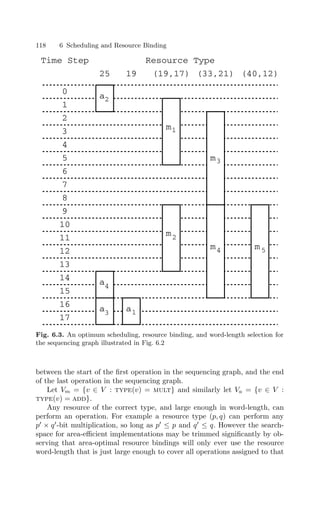
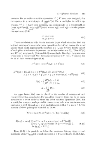
![120 6 Scheduling and Resource Binding
min(v) = min
r∈R(v)
L(r) (6.11)
max(v) = max
r∈R(v)
L(r) (6.12)
In order to bound the possible execution control steps of each operation,
it is necessary to utilize as-soon-as-possible (ASAP) and as-late-as-possible
(ALAP) scheduling [Par99], provided in Algorithms ASAP and ALAP for
completeness.
Algorithm 6.1
Algorithm ASAP
Input: A sequencing graph P(V, D) and a latency (v) for each operation v ∈ V
Output: A schedule S : V → N ∪ {0}
begin
mark(v) ← false for all v ∈ V
foreach v ∈ V : (v
, v) ∈ D do
S(v) ← 0
mark(v) ← true
end foreach
do
foreach v ∈ V : ∀(v
, v) ∈ D, mark(v
) = true do
S(v) ← max
(v,v)∈D
{S(v
) + (v
)}
mark(v) ← true
end foreach
while ∃v ∈ V : mark(v) = false
end
Algorithm 6.2
Algorithm ALAP
Input: A sequencing graph P(V, D), latency constraint λ, and
a latency (v) for each operation v ∈ V
Output: A schedule S : V → N ∪ {0}
begin
mark(v) ← false for all v ∈ V
foreach v ∈ V : ∃(v, v
) ∈ D do
S(v) ← λ − (v)
mark(v) ← true
end foreach
do
foreach v ∈ V : ∀(v, v
) ∈ D, mark(v
) = true do
S(v) ← min
(v,v)∈D
{S(v
)} − (v)
mark(v) ← true
end foreach
while ∃v ∈ V : mark(v) = false
end](https://image.slidesharecdn.com/optimizationandpreparationprocesses-240125021124-f0b0fb42/85/optimization-and-preparation-processes-pdf-133-320.jpg)
![6.3 Optimum Solutions 121
Consider performing ASAP and ALAP scheduling of the operations, using
a latency = min for all operations. Let asap(v) denote the resulting ASAP
control step for each operation v ∈ V . Similarly let alap(v, λ) denote the
ALAP control step for each operation v ∈ V given a user-specified latency
bound of λ and under the same operation latencies.
Each operation v ∈ V , executing on resource type r ∈ R(v), can only start
its execution during one of the time steps in the set T (v, r) (6.13).
T (v, r) = {t ∈ N∪{0} : t ≥ asap(v)∧t ≤ alap(v, λ)−L(r)+min(v)} (6.13)
It is useful to enumerate all possible start times T (v) for each operation
v ∈ V , according to (6.14), and indeed the complete set of time-steps T (6.15).
T (v) = {t|∃r ∈ R(v) : t ∈ T (v, r)} (6.14)
T = {t|∃v ∈ V : t ∈ T (v)} (6.15)
6.3.2 ILP Formulation
Extending the notation used by Landwehr, et al. [LMD94], the ILP may be
formulated as follows. Let bi,r define a Boolean variable with bi,r = 1 iff
instance number i of resource type r has at least one operation bound to it.
This allows the objective function to be formulated in linear form (6.16).
Minimize
r∈R
cost(r)
I(r)
i=1
bi,r (6.16)
In order to introduce the constraints, let xv,t,i,r be defined as in (6.17).
xv,t,i,r =
1, if operation v is scheduled at time-step t on the
ith instance of resource type r
0, otherwise
(6.17)
The minimization is performed subject to three types of constraint. The
first are the binding constraints, to ensure that each operation is executed
on exactly one instance (6.18). The second are the resource constraints, to
ensure that no resource instance is executing more than one operation at a
time (6.19). The final set are the precedence constraints, to ensure that all
operations obey the dependencies in the sequencing graph (6.20).
∀v ∈ V,
r∈R(v)
I(r)
i=1
t∈T (v,r)
xv,t,i,r = 1 (6.18)](https://image.slidesharecdn.com/optimizationandpreparationprocesses-240125021124-f0b0fb42/85/optimization-and-preparation-processes-pdf-134-320.jpg)
![122 6 Scheduling and Resource Binding
∀t ∈ T, ∀r ∈ R, ∀i ∈ {1, ..., I(r)},
v∈V :r∈R(v)
t1∈{t,...,t+L(r)−1}∩T (v,r)
xv,t1,i,r ≤ bi,r (6.19)
∀(v1, v2) ∈ D,
∀t ∈ T (v2) ∩ {asap(v1) + min(v1) − 1, . . . , alap(v1) + max(v1) − 1},
r∈R(v2)
I(r)
i=1
t2∈T (v2,r):t2≤t
xv2,t2,i,r +
r∈R(v1)
I(r)
i=1
t1∈T (v1,r):t1t−L(r)
xv1,t1,i,r ≤ 1
(6.20)
Example 6.5. Recall the simple sequencing graph of Fig. 6.2. The ILP formu-
lation for this sequencing graph contains 164 variables and 166 constraints for
λ = 18, the lowest achievable latency. Fig. 6.3 illustrates an optimal solution
corresponding to this latency constraint, which has the following optimiza-
tion variables taking the value 1: xa2,0,1,25, xa4,14,1,25, xa3,16,1,25, xa1,16,1,19,
xm1,1,1,(19,17), xm2,9,1,(19,17), xm3,2,1,(33,21), xm4,9,1,(33,21), xm5,9,1,(40,12), b1,25,
b1,19, b1,(19,17), b1,(33,21), b1,(40,12). All other variables are equal to zero.
After solution, the values of the ILP optimization variables xv,t,i,r and bi,r
encode a solution to Problem 6.3 given in (6.21–6.23).
Y = {(i, r) : bi,r = 1} (6.21)
R(v) =
r∈R(v)
I(r)
i=1
t∈T (v,r)
(i, r) · xv,t,i,r, for v ∈ V (6.22)
S(v) =
r∈R(v)
I(r)
i=1
t∈T (v,r)
t · xv,t,i,r, for v ∈ V (6.23)
Optimal solutions can only be found for relatively small examples using
ILP, due to the large number of variables and constraints. Moreover, the
number of variables and constraints increases linearly with the relaxation of
λ. It is these drawbacks that have motivated the search for efficient heuristic
solutions to this problem, as presented in Section 6.4.
6.4 A Heuristic Approach
This section presents a heuristic approach to Problem 6.3 [CCL01a]. The
proposed algorithm iteratively refines word-length information while using](https://image.slidesharecdn.com/optimizationandpreparationprocesses-240125021124-f0b0fb42/85/optimization-and-preparation-processes-pdf-135-320.jpg)
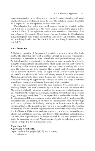
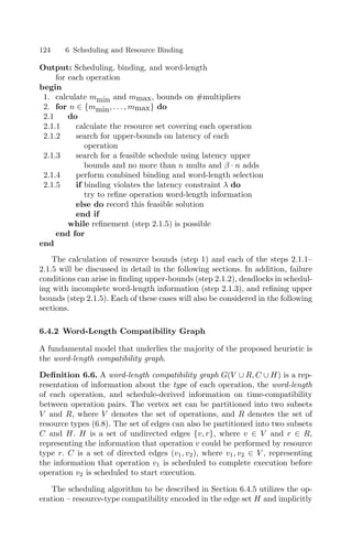
![6.4 A Heuristic Approach 125
creates the edge set C in the process. The combined binding and word-length
selection algorithm to be described in Section 6.4.6 utilizes both the time-
compatibility edge set C and the operation resource-type compatibility set
H.
It is important to note that the edge set C has been chosen to ensure that
subgraph G+
(V, C) exhibits a transitive orientation [Gol80], since if v1 ∈ V
finishes before v2 starts, and v2 finishes before v3 starts, it follows that v1
finishes before v3 starts. This orientation will be used in Section 6.4.6 to aid
fast resource binding. Note also that the set C of directed edges in the graph
need not be constructed explicitly in a software implementation, but can be
inferred from the scheduled times of the operations.
Example 6.7. A simple word-length compatibility graph is shown in Fig. 6.4(c),
corresponding to the data flow graph and schedule shown in Figs. 6.4(a) and
(b), respectively.
(a) sequencing graph
(c) wordlength
compatibility
graph
v1
MULT
(18,18)
v3
ADD
19
v2
MULT
(20,16)
v4
ADD
25
MULT
(20,16)
MULT
(20,18)
ADD
19
ADD
25
v1
v2
v3
v4
MULT
(18,18)
v1 v2
v3 v4
time
(b) schedule
Fig. 6.4. A Word-Length Compatibility Graph](https://image.slidesharecdn.com/optimizationandpreparationprocesses-240125021124-f0b0fb42/85/optimization-and-preparation-processes-pdf-138-320.jpg)
![126 6 Scheduling and Resource Binding
The initial word-length compatibility graph is constructed in the following
manner: A resource set R is constructed following (6.5–6.8). Edge set H is
initialized to the set {{v ∈ V, r ∈ R} : r ∈ R(v)}. C is initialized to the empty
set. As Algorithm ArchSynth executes, word-length refinement will result in
the deletion of edges from the set H.
6.4.3 Resource Bounds
The first stage of the heuristic is to find the smallest and largest sensible
upper bounds to place on the number of multipliers required. These values are
obtained from a study of how the iteration latency achieved by list-scheduling
decreases with the number of multipliers allowed.
A standard resource-constrained list scheduling algorithm [DeM94, NT86]
can be used to heuristically obtain these bounds. Standard ALAP urgency-
based list scheduling with a bound c ∈ N2
on the number of resources of each
type is used. c is a 2-vector of integer elements, the first corresponding to
the bound on the number of multipliers and the second corresponding to the
bound on the number of adders.
The bounds mmin and mmax used in Algorithm ArchSynth can now be
defined, assuming that the given latency bound is realizable. Bound mmin is
the smallest value such that the list-scheduled latency is within the constraint
for all schedules with c ≥ (mmin, βmmin) and (v) = min(v) for all v ∈
V . Similarly bound mmax is the smallest value such that the list-scheduled
latency is within the constraint for all schedules with c ≥ (mmax, βmmax)
and (v) = max(v) for all v ∈ V . For tight latency constraints there may
be no such mmax value, in which case mmax is set to |Vm|. In each of these
cases, a binary search is used to determine the bounds.
The rationale behind these bounds is the following. If an algorithm can-
not be scheduled to meet the imposed latency constraint under a resource
constraint c, even when all operations have their minimum possible latency,
then the algorithm cannot meet this latency constraint for any c
≤ c. This
provides a lower bound on the number of each type of resource required. Sim-
ilarly, if the imposed timing constraint can be met under a resource constraint
c, even when all operations have their maximum latency, then the algorithm
can meet this latency constraint for all c
≥ c. This provides an upper bound
on the number of each type of resource required. Fig. 6.5 illustrates the way in
which the achieved latency varies with the bound on the number of multipliers
supplied to the list-scheduler.
Example 6.8. An example derivation of resource bounds is illustrated in
Fig. 6.6. Fig. 6.6(a) illustrates a simple data flow graph, with correspond-
ing initial word-length compatibility graph shown in Fig. 6.6(b). The latency
curves resulting from list scheduling for different resource bounds are plotted
in Fig. 6.6(c). The points corresponding to the minimum possible number and
maximum necessary number of multiplier resources have been highlighted.](https://image.slidesharecdn.com/optimizationandpreparationprocesses-240125021124-f0b0fb42/85/optimization-and-preparation-processes-pdf-139-320.jpg)
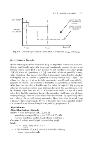
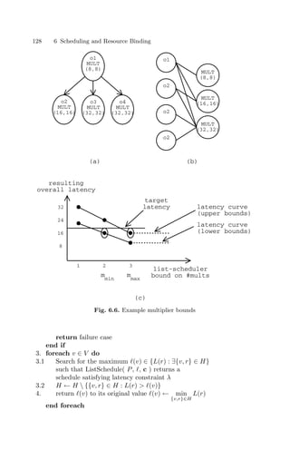
![6.4 A Heuristic Approach 129
end
Using Algorithm LatencyBounds, an upper bound on the latency of each
operation can be established. Once this has been done, the set of edges H
of the Word-Length Compatibility Graph, representing the possible design
decisions, has been pruned.
6.4.5 Scheduling with Incomplete Word-Length Information
At the time of scheduling in Algorithm ArchSynth, the word-length of each
operation may not be fixed. Indeed each operation could be implemented
using any resource type to which the operation is linked by an edge in the
word-length compatibility graph. The scheduling problem therefore has in-
completely defined constraints [CSH00], and a technique must be developed
to incorporate these constraints into directing the search for a solution. The
following paragraphs illustrate the need for such a technique, before introdu-
cing the proposed solution.
Traditional resource-constrained scheduling techniques such as force-directed
list scheduling [PK89], require resource constraints to be expressed in terms of
a bound on the number of resources of each type. During standard list schedul-
ing, these constraints are tested at each time step before deciding whether to
schedule a new operation. The constraints may be formally expressed as fol-
lows. Let ev,t be defined as in (6.24). Thus ev,t = 1 iff operation v is executing
during time-step t. Given a set of control steps T (6.15), a set of operations V ,
and the maximum number of resources ck of type k, the traditional resource
constraints may be expressed as (6.25).
ev,t =
1, if (S(v) ≤ t) ∧ (S(v) + (v) t)
0, otherwise
(6.24)
∀k ∈ {add, mult}, max
t∈T
v∈V :type(v)=k
ev,t ≤ ak (6.25)
In the case of multiple word-length systems, these constraints tend to be
too relaxed to guarantee that no more than ak resources of type k will be used
by the given schedule.
Example 6.9. Consider the schedules and corresponding word-length compat-
ibility graphs shown in Fig. 6.7. Such graphs could arise during the execution
of Algorithm ArchSynth. Fig. 6.7(a) has fully defined word-length information
for each operation. It is clear that even though v1, v2 and v3 are all multiplic-
ations and do not overlap in execution, three distinct multiplier resources will
still be required for their implementation. However the standard scheduling
constraint (6.25) would be satisfiable for amult = 1.
Fig. 6.7(b) has an incomplete specification (there is at least one operation
which could be implemented in more than one possible resource type). How-
ever a 32 × 32-bit multiplier could conceivably implement every operation.](https://image.slidesharecdn.com/optimizationandpreparationprocesses-240125021124-f0b0fb42/85/optimization-and-preparation-processes-pdf-142-320.jpg)
![130 6 Scheduling and Resource Binding
(a) fully specified
wordlength information
(b) incomplete specification
(full sharing possible)
(c) incomplete specification
(general case)
v
time
3
v2
v1
MULT
(32,32)
MULT
(16,16)
v
MULT
(16,16)
v
MULT
(32,32)
2
3
v
MULT
(8,8)
1
MULT
(8,8)
MULT
(32,32)
MULT
(16,16)
v
MULT
(16,16)
v
MULT
(32,32)
2
3
v
MULT
(8,8)
1
MULT
(8,8)
v
time
3
v2
v1
MULT
(32,32)
MULT
(16,16)
v
MULT
(16,16)
v
MULT
(32,32)
2
3
v
MULT
(8,8)
1
MULT
(8,8)
v
time
3
v2
v1
Fig. 6.7. Some schedules and word-length compatibility graphs
Thus it is possible to implement the entire system using a single multiplier
resource.
Fig. 6.7(c) illustrates a general case, corresponding to the deletion of a
single edge from the word-length compatibility graph of Fig. 6.7(b). Using
traditional methods, it is unclear in this case how to incorporate such con-
straints into the search for an appropriate schedule.
These examples demonstrate that a more sophisticated approach to schedul-
ing is required to take word-length information into account. In general it is
necessary to consider the incomplete word-length specification provided by an
edge set H.
The scheduling algorithm proposed is a modification of standard list
scheduling [DeM94]. The modification lies in the resource constraint calcu-
lation. Before any scheduling takes place, a small cardinality subset S ⊆ R
is found such that ∀v ∈ V, ∃s ∈ S : {v, s} ∈ H. Conceivably, a resource
binding could consist only of resource of types represented in S. Define
O(r) to be the set of operations performable by resource type r ∈ R,
i.e. O(r) = {v ∈ V : ∃{v, r} ∈ H}. Similarly let S(v) denote the sub-
set of resource types in S which could implement operation v ∈ V , i.e.
S(v) = {s ∈ S : ∃{v, s} ∈ H}. Then the proposed constraint function to
be used in the algorithm can be expressed as in (6.26).
∀k ∈ {add, mult},
s∈S:type(s)=k
max
t∈T
v∈O(r)
ev,t|S(v)|−1
≤ ak
(6.26)
This is a heuristic measure with the following justification. Firstly (6.26)
is at least as strict as (6.25), which is a special case of the former under the
condition |type(V )| = |S|, the smallest sized S possible. This represents the](https://image.slidesharecdn.com/optimizationandpreparationprocesses-240125021124-f0b0fb42/85/optimization-and-preparation-processes-pdf-143-320.jpg)
![6.4 A Heuristic Approach 131
case where each multiplication could be performed by a single large multi-
plier, and each addition could be performed by a single large adder. As the
possibilities for the implementation of each operation are reduced during ex-
ecution of Algorithm ArchSynth, the balance on the left hand side of (6.26)
shifts from the max
t∈T
to the
s∈S
to reflect the stricter constraints. The small
cardinality S is used in order to relax the constraint as much as possible, since
any two operations in O(s) could possibly be eventually bound to the same
resource. Operations belonging to more than one O(s), i.e. those v ∈ V with
|S(v)| 1, are accounted for by ‘sharing’ equally their usage between each of
the elements S(v).
Algorithm IncompSched illustrates this scheduling based on incomplete
information. Two auxilliary data structures are used in the algorithm to keep
track of the scheduling constraint (6.26), usage(s) and maxusage(s). Respect-
ively, these keep track of the instantaneous and peak usage of resource type
s ∈ S. The algorithm starts by setting the latency (v) of each operation
to its maximum (step 1). After so doing, a standard ALAP-based urgency
measure [DeM94] is calculated for each node (step 2), and the time step in-
dex is initialized (step 3). The set S described above (step 4), and its related
function S(v) (step 5), to be used in the scheduling constraint (6.26) are then
calculated. Step 6 ensures that the peak usage maxusage(s) for each element
of that set is initialized. The algorithm then enters its main scheduling loop,
with one iteration per time step (step 7).
At the start of each iteration, the instantaneous usage of resources is initial-
ized (step 7.1), the ready-list is calculated (step 7.2), and the prime candidate
for scheduling is selected (step 7.3). The algorithm then enters a secondary
loop (step 7.4), which tries to schedule this and any other operation of the
same type. The current left-hand side of (6.26) is first calculated (step 7.4.1),
and then updated (step 7.4.2) for any s ∈ S for which scheduling in the cur-
rent control step would use more than the current peak usage for that s. If
the updated (6.26) is still satisfied, then the scheduling of the operation is ac-
cepted (step 7.4.3), and the peak usage is updated (step 7.4.4). Deadlocks, to
be discussed below, may occur in the scheduling process. These are detected
by step 7.5.
Example 6.10. An example execution of Algorithm IncompSched is shown in
Fig. 6.8. The data flow graph and word-length compatibility graph are shown
in Figs. 6.8(a) and (b) respectively. Fig. 6.8(c) enumerates the S(v) sets for
this example, and Fig. 6.8(d) shows how the usage and maxusage variables
evolve as the algorithm executes for aadd = 1, amult = 2. The resulting
schedule is shown in Fig. 6.8(e), and could be resource-bound as a single
16-bit adder together with both a 16 × 16-bit multiplier and a 32 × 32-bit
multiplier. Details on how such a resource binding can be found for general
graphs are discussed in the following section.](https://image.slidesharecdn.com/optimizationandpreparationprocesses-240125021124-f0b0fb42/85/optimization-and-preparation-processes-pdf-144-320.jpg)
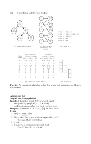
![6.4 A Heuristic Approach 133
5. Let S(v) = {s ∈ S : ∃{v, s} ∈ H}
6. maxusage(s) ← 0 for all s ∈ S
7. do
7.1 usage(s) ← 0 for all s ∈ S
7.2 E ← the list-schedule ‘ready list’ [DeM94], sorted by urgency
7.3 e ← most urgent element of E
7.4 do
7.4.1 total ←
s∈S({v∈V :type(v)=type(e)})
maxusage(s)
7.4.2 foreach s ∈ S(e):
usage(s) + |S(e)|−1
maxusage(s) do
total ← total − maxusage(s)+
usage(s) + |S(e)|−1
end foreach
7.4.3 if total ≤ atype(e) do
S(e) ← t
usage(s) ← usage(s) + |S(e)|−1
7.4.4 foreach s ∈ S(e) : usage(s) maxusage(s) do
maxusage(s) ← usage(s)
end foreach
end if
7.4.5 e ← next most urgent element of E, if one exists
while such an e exists ∧ ∃k ∈ {add, mult} :
s∈S:type(s)=k
maxusage(s) ai
t ← t + 1
7.5 if deadlock detected do
return failure case
end if
while there remains at least one unscheduled operation
end
There are a number of significant differences between standard list schedul-
ing and Algorithm IncompSched. Information on resource usage is accumu-
lated over control steps in Algorithm IncompSched, rather than each step
being constraint-function-independent of each other step. There are two re-
lated drawbacks from this: Firstly, it is possible for the proposed list-scheduler
to deadlock, by scheduling operations belonging to O(s1) for the some s1 ∈ S
early in the schedule and then having no remaining resources to schedule
operations belonging to O(s2) for some s2 ∈ S, s2 = s1 later in the sched-
ule. Such deadlocks can be easily detected: if all operations have finished by
the current time-step and yet no operation has been scheduled by the end of
that time-step, deadlock has occurred. Secondly, although the scheduler may
not deadlock, greedy allocation of parallel O(s1) operations early-on in the
schedule may cause schedules of longer than optimal latency. Thus Algorithm
IncompSched has a greedy bias towards earlier time steps.](https://image.slidesharecdn.com/optimizationandpreparationprocesses-240125021124-f0b0fb42/85/optimization-and-preparation-processes-pdf-146-320.jpg)
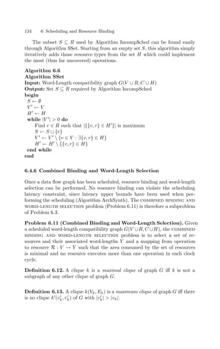
![6.4 A Heuristic Approach 135
Definition 6.14. A clique k(v
, c
) of the subgraph G+
(V, C) of word-length
compatibility graph G(V ∪ R, C ∪ H) is a feasible clique iff ∃r ∈ R : ∀v ∈
v
, {v, r} ∈ H.
The combined binding and word-length selection problem is ap-
proached by partitioning the subgraph G+
(V, C) into a set K of feasible
cliques. The feasibility constraint captures the requirement that there must
be a single resource capable of performing all operations in the clique. The
cost of this resource binding is then given by (6.27).
k(vk,ek)∈K
min
r∈R:∀v∈vk,∃{v,r}∈H
cost(r) (6.27)
This problem is a special case of the set-covering or weighted unate cov-
ering problem.
Problem 6.15 (SET COVERING, [Chv79]). Consider a set of sets U =
{u1, u2, . . . , un} and associated positive costs cu1 , cu2 , . . . , cun . Let I =
%
u∈U
u.
A subset U
⊆ U is a cover iff
%
u∈U
u = I. The cost of this cover is
u∈U
cu.
The problem is to find a cover of minimum cost.
The combined binding and word-length selection problem can be cast as a
set covering problem in the following manner. Let U denote the set of node sets
of all feasible cliques in the graph G+
(V, C) (6.28). The cost ck associated with
clique k ∈ U is given by the corresponding term in the summation of (6.27).
U = {V
⊆ V : V
induces a feasible clique in G+
(V, C)} (6.28)
The proposed approach is to extend a known heuristic for solving the
unate covering problem [Chv79] to the combined resource binding and word-
length selection application. In order to present the proposed extensions to
this simple heuristic, it is first reviewed below.
Intuitively, for a greedy algorithm it becomes more desirable to include
a set uj in the cover U
as the number of elements covered by uj and not
already covered by any previously chosen set increases. This is tempered by
the cost of set uj, and thus the ratio of these two quantities forms an appro-
priate measure of desirability. This observation leads to the following heuristic
proposed in [Chv79].
Algorithm 6.7
Algorithm ChvatalHeur
Input: An instance of the set covering problem (problem 6.15)
Output: A cover U
⊆ U
begin
U
← ∅](https://image.slidesharecdn.com/optimizationandpreparationprocesses-240125021124-f0b0fb42/85/optimization-and-preparation-processes-pdf-148-320.jpg)
![136 6 Scheduling and Resource Binding
while ∃i : |ui| = 0 do
find i such that |ui|/ci is maximum
U
← U
∪ {ui}
foreach j ∈ {1, . . . , n} do
uj ← uj ui
end foreach
end while
end
The first, and simplest, extension to [Chv79] is to include some compens-
ation for the greedy nature of the original algorithm. If a clique is chosen
during one iteration of the algorithm, it is checked whether this clique could
be extended to cover all operations covered by any of the cliques chosen at pre-
vious iterations. If such an extension is possible, the selected clique is grown
accordingly and the previously chosen clique is deleted from the cover set.
The more important distinction is that the set U is never calculated, since
its size can be very large (exponential in |V |). Instead, an implicit approach
is used, which is polynomial in |V |.
Consider the set of clique node-sets Ur ⊆ U that may be implemen-
ted using a resource r ∈ R, i.e. Ur = {u ∈ U : ∀v ∈ u, {v, r} ∈ H}. It
is clear that it only makes sense to select those cliques induced by max-
imal subsets u ∈ Ur : u
∈ Ur : u ⊂ u
for implementation in resource
type r. Non-maximal cliques correspond to so-called ‘column domination’ in
unate covering [GN72]. However a stronger statement can be made, that
only maximum feasible cliques need to be considered as candidates, i.e.
u ∈ Ur : u
∈ Ur : |u| |u
|. This is because Chvatal’s heuristic [Chv79]
will always return a higher score for a maximum feasible clique than for a
non-maximum clique of the same resource type, and so a maximum clique
will always be chosen in preference to a non-maximum clique. Incorporat-
ing this knowledge leads to the proposed resource binding and word-length
selection algorithm presented below as Algorithm ResBindWLSel.
The algorithm starts by initializing certain values (steps 1–4). In step 1,
C is set to correctly reflect its definition (Table A). V1 is initialized to the full
set of operations (step 2), and will be iteratively reduced as operations are
bound to resources (step 5.7). nr is a counter of how many resources of type
r ∈ R have thus far been allocated by the binding, and is initialized to 0 (step
3). Y , the final set of resources, is initialized to be empty (step 4).
After initialization, the algorithm enters its main loop (step 5), where
one resource type is selected, and operations bound to an instance of that
resource type, on each iteration. In order to choose which resource type to
select, Chvatal’s heuristic is applied (steps 5.1–5.2). Compensation for the
greedy nature of this heuristic is provided by step 5.3, which can backtrack
on previous decisions, as described above. Finally, steps 5.4–5.7 perform the
binding: step 5.4 adds a new resource to the existing set, step 5.5 binds each
operation in the clique selected by steps 5.1–5.2 to this new resource. Finally,](https://image.slidesharecdn.com/optimizationandpreparationprocesses-240125021124-f0b0fb42/85/optimization-and-preparation-processes-pdf-149-320.jpg)
![6.4 A Heuristic Approach 137
the number of resources of that type is incremented (step 5.6) and the set of
unbound operations is reduced (step 5.7).
Algorithm 6.8
Algorithm ResBindWLSel
Input: A Word-Length Compatibility Graph
G(V ∪ R, C ∪ H) and schedule S : V → N ∪ {0}
Output: A resource set Y and a binding R : V → Y
begin
1. C ← {(v1, v2) : v1, v2 ∈ V ∧ S(v1) + max
{v1,r}∈H
L(r) ≤ S(v2)}
2. V1 ← V
3. nr ← 0 for all r ∈ R
4. Y ← ∅
5. while |V1| 0 do
5.1 foreach r ∈ R do
V
← {v ∈ N : ∃{v, r} ∈ H}
Let G
(V
, E
) be the subgraph of G+
(V, C)
induced by vertex set V
Search G
(V
, E
) for a maximum clique with
node set pr ⊆ V
end foreach
5.2 Choose r ∈ R such that |pr|(cost(r))−1
is maximum
5.3 foreach y ∈ Y
V
← {v ∈ V : R(v) = y}
if ∀v ∈ V
: ∃{v, r} ∈ H and V
∪ pr induces a
clique in G+
(V, C) do
Y ← Y {y}
R(v) ← (r, nr) for all v ∈ y
end if
end foreach
5.4 Y ← Y ∪ {(r, nr)}
5.5 R(v) ← (r, nr) for all v ∈ pr
5.6 nr ← nr + 1
5.7 V1 ← V1 pr
end while
end
Because the graph G+
(V, C) (and any subgraph induced by a vertex sub-
set) is a transitively oriented graph, finding the maximum clique is a simple
linear-time operation [Gol80].
Example 6.16. Consider the data flow graph illustrated in Fig. 6.9(a). An ex-
ample execution of Algorithm ResBindWLSel is illustrated in Fig. 6.9(d-f) for
the schedule and word-length compatibility graph shown in Fig. 6.9(b) and
(c). Three iterations are required. During the first iteration, a 30-bit adder
is selected to perform operations v2 and v3. The second iteration selects a](https://image.slidesharecdn.com/optimizationandpreparationprocesses-240125021124-f0b0fb42/85/optimization-and-preparation-processes-pdf-150-320.jpg)
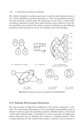
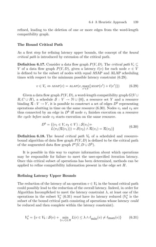
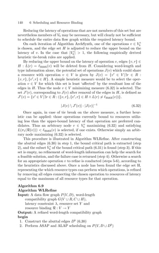
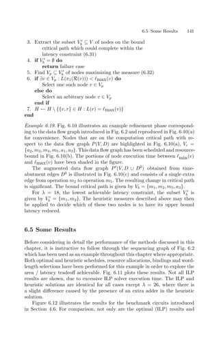
![142 6 Scheduling and Resource Binding
m
MULT
(18,15)
m
MULT
(19,17)
m
MULT
(33,21)
m
MULT
(22,16)
m
MULT
(40,12)
a
ADD
25
a
ADD
22
a
ADD
19
1
2 3
4 5
1 3
4
m
MULT
(18,15)
m
MULT
(19,17)
m
MULT
(33,21)
m
MULT
(22,16)
m
MULT
(40,12)
a
ADD
20
a
ADD
25
a
ADD
22
a
ADD
19
1
2 3
4 5
1
2
3
4
0
2
4
6
8
10
12
14
16
18
20
22
24
26
m 1
m 2
m3
m4
a2
a4
a1
a3
ADD
25
MULT
(40,17)
MULT
(33,21)
a
ADD
20
2
m5
critical
node
min
operation
latency
max
operation
latency
(a) sequencing graph (b) initial schedule
(c) augmented sequencing graph
Fig. 6.10. Example use of the bound critical path for word-length refinement
the heuristic results provided, but also the solutions corresponding to word-
length-blind scheduling followed by an optimal resource binding [CCL00b]. All
three sets of results are only provided for the IIR filter, the polyphase filter
bank and the RGB to YCrYb convertor, due to the excessive execution time
of both the ILP solver and the optimal binding.
These results illustrate that for the benchmark circuits, the heuristic
presented in this chapter provides a significant improvement in area (between
−16% and 46%, average 15%) over a two-stage approach of scheduling and
then binding, even when the binding is optimal. The heuristic results have
between 0% and 62% (average 14%) worse area than the optimum combined
solution, for cases where the optimum is known.
In order to fully characterize the heuristic performance, further results
have been obtained using artificially generated examples. For statistically sig-
nificant data on solution quality, 200 random sequencing graphs have been](https://image.slidesharecdn.com/optimizationandpreparationprocesses-240125021124-f0b0fb42/85/optimization-and-preparation-processes-pdf-155-320.jpg)
![6.5 Some Results 143
15 20 25 30 35 40 45
800
900
1000
1100
1200
1300
1400
1500
1600
latency constraint λ
resulting
area
heuristic synthesis
optimal (ILP) synthesis
Fig. 6.11. Design-space exploration for the simple sequencing graph of Fig. 6.2
generated for each (problem size |V |, latency constraint λ) pair, using a variant
of the TGFF algorithm [DRW98]. The first set of detailed quality results that
has been collected, measures the variation of the heuristic solution quality with
both the problem size and the tightness of the supplied latency constraint. For
each sequencing graph, the minimum possible latency constraint λmin has
been found using ASAP scheduling, from which latency constraints have been
generated corresponding to a 0% to 30% relaxation of λmin. Algorithm Arch-
Synth has then been executed on the graph / latency constraint combination.
The resulting area has been normalized with respect to the optimal solution
resulting from [CCL00b] where operations may only share resources when the
implemented resource has latency no longer than the minimum required to
implement the given operations. These results are plotted in Fig. 6.13, as a
percentage area penalty for using the approach of [CCL00b] over the heuristic
presented in this chapter. Each point represents the mean of two hundred
representative designs.
The results illustrate that for designs with even a small ‘slack’ in terms
of latency constraints, significant area improvements of up to 30% can be
made by performing the scheduling, binding, and word-length selection in the
intertwined manner proposed. The area improvements come from increased
resource sharing due to implementing small word-length operations in larger](https://image.slidesharecdn.com/optimizationandpreparationprocesses-240125021124-f0b0fb42/85/optimization-and-preparation-processes-pdf-156-320.jpg)
![144 6 Scheduling and Resource Binding
13 13.5 14 14.5 15 15.5 16 16.5 17 17.5 18
250
300
350
400
450
500
550
600
650
700
λ
area
optimal (ILP)
heuristic
optimal binding from [CCL00b]
7 8 9 10 11 12 13 14
3000
3500
4000
4500
5000
5500
6000
6500
7000
7500
λ
area
heuristic
optimal binding from [CCL00b]
(a) IIR (b) FIR
14 15 16 17 18 19 20 21
450
500
550
600
650
700
750
800
850
λ
area
heuristic
14 15 16 17 18 19 20 21
400
450
500
550
600
650
700
750
λ
area
heuristic
(c) DCT1
(d) DCT2
5 5.5 6 6.5 7 7.5 8 8.5 9 9.5 10
100
110
120
130
140
150
160
170
180
190
200
λ
area
optimal (ILP)
heuristic
optimal binding from [CCL00b]
13 13.5 14 14.5 15 15.5 16 16.5 17 17.5 18
80
90
100
110
120
130
140
150
160
170
λ
area
optimal (ILP)
heuristic
optimal binding from [CCL00b]
(e) PFB (f) RGB–YCrCb
Fig. 6.12. Design-space exploration for the benchmark circuits of Section 4.6](https://image.slidesharecdn.com/optimizationandpreparationprocesses-240125021124-f0b0fb42/85/optimization-and-preparation-processes-pdf-157-320.jpg)
![6.5 Some Results 145
0
5
10
15
20
25
0
5
10
15
20
25
30
−5
0
5
10
15
20
25
30
No. operations
Latency constraint
Area
penalty
(%)
Fig. 6.13. Variation with number of operations and latency constraint of area
penalty for [CCL00b] over the proposed heuristic
word-length resources with longer latency. Even for relatively small graphs,
area improvements of tens of percent are possible.
Fig. 6.14 illustrates the increase in implementation area from using the
heuristic presented in Section 6.4 over the optimum combined problem presen-
ted in Section 6.3. These results can only be provided for modest problem size
and a minimum latency constraint λ = λmin, as the ILP solution execution
time scales rapidly with problem size and as the latency constraint is relaxed.
The variation of minimum-latency execution time with problem size for
200 graphs using the ILP model (solved with lp solve [Sch97] on a Pentium
III 450MHz) and the heuristic algorithm (implemented in C on the same
machine) is shown in Fig. 6.15, illustrating the polynomial complexity of the
heuristic against the exponential complexity of the ILP. Over the range of 1 to
10 operations, the relative increase in area ranges from 0% to 16% whereas the
ILP solution takes between one and three orders of magnitude greater time
to execute. An important point not brought out by these results is the scaling
of execution time with overall latency constraint. The number of variables
in the ILP model scales with the latency constraint, making the execution
time highly dependent on this parameter. This is illustrated in Table 6.1
for 200 9-operation sequencing graphs. By contrast, the execution time of
Algorithm ArchSynth does not scale with the latency constraint. Thus the](https://image.slidesharecdn.com/optimizationandpreparationprocesses-240125021124-f0b0fb42/85/optimization-and-preparation-processes-pdf-158-320.jpg)
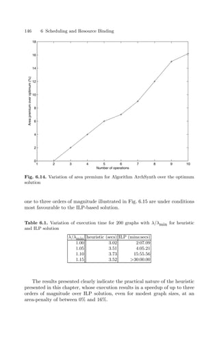
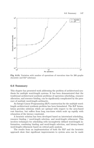

![7
Conclusion
This final chapter contains two sections. Section 7.1 summarizes the key ideas
in this book, while Section 7.2 contains suggestions for future work.
7.1 Summary
This book has examined the problems surrounding the synthesis of hardware
from initial infinite precision specifications of DSP algorithms. Such a syn-
thesis procedure raises the level of abstraction at which a DSP algorithm can
be specified, to the level typically used by DSP algorithm designers.
As a result of investigating efficient DSP implementation architectures, it
has been argued that the multiple word-length paradigm can result in efficient
implementations, incorporating fine control in the trade-off of implementation
area and power consumption against acceptable arithmetic error. The term
lossy synthesis has been coined to describe the incorporation such a trade-off
within the synthesis process itself.
The design and development of multiple word-length systems is not a
simple process; indeed it has been proven that the search for optimal archi-
tectures is an NP-hard problem [CW01]. However an heuristic algorithm has
been presented, which achieves significant improvements of up to 45% in area
and 39% in speed, compared to traditional design techniques which consider
only a single uniform system word-length for all the signals in the system.
Different approaches to the problem of overflow have been considered. Im-
plementations making use of saturation arithmetic have been compared to
systems scaled to ensure that no overflow is possible. A technique has been
introduced to automate the design of saturation arithmetic systems. The pro-
posed technique automates the placement of each saturation nonlinearity and
the degree of saturation at each nonlinearity. Results indicate that up to a
further 8% reduction in system area and 24% speedup can be achieved by
applying saturation automation techniques together with the multiple word-
length approach described above. The relative advantage of saturation arith-](https://image.slidesharecdn.com/optimizationandpreparationprocesses-240125021124-f0b0fb42/85/optimization-and-preparation-processes-pdf-162-320.jpg)
![150 7 Conclusion
metic is shown, however, to depend heavily on the nature of the algorithm to
which it is applied.
Finally, the impact of multiple word-length designs on architectural syn-
thesis has been assessed. Optimal and heuristic techniques have been proposed
for the combined problem of scheduling, resource allocation, word-length se-
lection, and resource binding for multiple word-length synthesis. The proposed
approaches allow a wide design-space to be searched, trading off the number
of samples processed per clock period against implementation area. Compared
to previous techniques which do not take into account the variation of oper-
ation latency with word-length, our approach can achieve area savings of up
to 46%.
7.2 Future Work
There are many ways in which the work presented in this book could be taken
forward and expanded to new domains, new architectures, and new objectives.
In this section some of the possibilities will be expanded upon.
The objective functions used throughout this book have concentrated on
the minimization of implementation area. Often the resulting circuits have
displayed a significant increase in maximum clock frequency and reduction
in power consumption as desirable side-effects of the optimization techniques
used. However it may be useful in the future to explicitly consider clock fre-
quency or power consumption within the objective function or as a constraint
on the optimizations performed. In synchronous systems the maximum allow-
able clock frequency is determined by worst-case propagation delay, whereas
area has, in this book, been modelled by a weighted sum of different compon-
ent areas. It is likely that this difference in the nature of the objective function
would require further development of the optimization algorithms.
As discussed in Chapter 6, performing word-length optimization before
architectural synthesis can lead to sub-optimal designs. A future direction of
research would be to investigate the interdependence between these two steps
and to develop a combined architectural synthesis and word-length optimiza-
tion approach. Some steps in this direction have recently been made by Kum
and Sung [KS01].
Dynamic reconfiguration is an area of particular interest in the FPGA
community [SLC98]. This term refers to ‘on-the-fly’ modifications to the hard-
ware encoded in an FPGA configuration. Bondalapati, et al. have proposed
a technique to vary the word-length of a loop variable over time, as the loop
executes [BP99]. Another avenue for future research would be to concentrate
on the extension of the framework described in this book to time-evolution of
precision requirements.](https://image.slidesharecdn.com/optimizationandpreparationprocesses-240125021124-f0b0fb42/85/optimization-and-preparation-processes-pdf-163-320.jpg)
![A
Notation
This appendix introduces some of the background notation and definitions,
which are used throughout the book.
A.1 Sets and functions
Z is used to denote the set of all integers. N is similarly the set of all natural
numbers (positive integers). R is used to denote the set of all reals.
f : X → Y denotes a function mapping elements of X to elements of Y . In
this context f(X) ⊆ Y denotes the range of function f.
Following a notation commonly used in DSP texts, square brackets ([ and ])
are used throughout the thesis when it is useful to distinguish a function with
a discrete domain from a function with a continuous domain (for which round
brackets are used). Thus for f1 : R → R we write f1(x), but for f2 : Z → R
we write f2[k].
∪ is used to denote the union of sets and ∩ to denote their intersection.
|X| is used to denote the size (cardinality) of a set X
X × Y denotes the Cartesian product of the sets X and Y
A.2 Vectors and Matrices
Vectors are denoted with bold face and their elements with subscripts, thus
ai is the i’th element of vector a
AT
denotes the transpose of a matrix A, whereas AH
denotes the conjugate
transpose.
Definition A.1. Let a and b be two vectors a, b ∈ Rn
. The vector relation
a ≤ b ⇔ ai ≤ bi for all 1 ≤ i ≤ n. Similarly a b ⇔ ∃i : ai bi.](https://image.slidesharecdn.com/optimizationandpreparationprocesses-240125021124-f0b0fb42/85/optimization-and-preparation-processes-pdf-164-320.jpg)
![152 A Notation
A.3 Graphs
Definition A.2. A directed graph G(V, E) consists of a finite set V and an
irreflexive binary relation E ⊂ V × V on V . An element of V is referred to as
a vertex or node. An element of E is referred to as an edge.
Definition A.3. For a graph G(V, E), inedge(v) (outedge(v)) is used to de-
note the set of in-edges (out-edges) {(v
, v) ∈ E} ({(v, v
) ∈ E}).
Definition A.4. The indegree (outdegree) of the node v ∈ V of a graph
G(V, E) is the size of the node’s inedge (outedge) set.
Definition A.5. For a graph G(V, E), pred(v) (succ(v)) is used to denote the
set of predecessor (successor) nodes {v
: (v
, v) ∈ E} ({v
: (v, v
) ∈ E}).
A.4 Miscellaneous
z∗
denotes the conjugate of a complex number z.
∧ is used to denote the logical (Boolean) and function
∨ is used to denote the logical (Boolean) or function
Definition A.6. The z-transform of a sequence h[t] is written Z{h[t]} as
defined in (A.1). The inverse z-transform of a function H(z) is written
Z−1
{H(z)}.
Z{h[t]} =
∞
t=−∞
h[t]z−t
(A.1)
A.5 Pseudo-Code
This section provides a brief description of the pseudo-code used. Keywords
are given in bold. There are 14 keywords: Input, Output, begin, while,
end, do, foreach, if, switch, case, for, goto, and, and return.
Each algorithm begins with an Input and Output line describing the
pre-requisites for and results of algorithm execution, respectively. The body
of the algorithm is enclosed within begin–end delimiters.
The while, do, if, switch, case, for, goto and return keywords are
taken directly from C [KR78]. foreach allows iteration over each member of
a set. A label ‘L1’ for a goto is indicated by ‘L1:’ preceding the labelled line
of code.
while, if, or foreach constructs containing more than one line of code are
enclosed within do–end delimiters.](https://image.slidesharecdn.com/optimizationandpreparationprocesses-240125021124-f0b0fb42/85/optimization-and-preparation-processes-pdf-165-320.jpg)
![154 A Notation
control step: The basic unit of time used in scheduling. A control step is equal
to a state in finite state machine-based controllers or to a microprogram
step in microprogrammed control units [Cam90].
cross-correlation: See Definition 5.5, p. 84.
DAG: Directed acyclic graph.
data-dependencies: An operation x is data-dependent on an operation y if y
produces a result which is consumed by x. For example the code frag-
ment a = b + c; d = a * b; contains a data-dependency between the
multiplication operation and the addition operation [ASU86].
data path: The part of a design that deals with computation of data. Data
paths are often characterized by regular logic and bit slices, for example
ALUs and adders [Cam90].
DCT: Discrete Cosine Transform [Mit98].
direct form: Several filter implementation structures come under the banner
of ‘direct form’ implementations. These are discussed in detail in [Mit98],
Chapter 6.
directed graph: See Definition A.2, p. 152.
DSP: Digital Signal Processing.
finite state machine: A machine defined by a finite set of states S, a set of pos-
sible input vectors I, a set of possible output vectors O, a state transition
function f : I × S → S, and an output function g : I × S → O.
FIR: Finite Impulse Response.
fixed-point: A binary representation for numbers [Kor02].
floating-point: A binary representation for numbers [Kor02].
genetic algorithm: A heuristic search technique based on biological evolu-
tion [RSORS96].
iff: If and only if.
iid: Independent, Identically Distributed.
IIR: Infinite Impulse Response.
injection input: A conceptual device used to model finite precision represent-
ation errors through a linearization process. Injection inputs are discussed
in Sections 3.1.1 and 4.1.2.
intractable: An intractable problem is one that is unsolvable by any polyno-
mial time algorithm [GJ79].
kurtosis: The fourth order statistical moment [Chu74].
latency: The latency of a resource is equal to the number of clock cycles
elapsing between presentation of the inputs to the resource, and the result
appearing at the output of the resource. The latency of an algorithm is
the number of clock cycles elapsing between the start of the first operation
in the algorithm and the end of the last operation in the algorithm.
loop: See Definition 2.3, p. 11.
LSB: Least Significant Bit.
LTI: Linear Time Invariant.
MSB: Most Significant Bit.](https://image.slidesharecdn.com/optimizationandpreparationprocesses-240125021124-f0b0fb42/85/optimization-and-preparation-processes-pdf-167-320.jpg)
![A.5 Pseudo-Code 155
NP-hard: Any problem which to which an NP-complete problem may be re-
duced in polynomial time [GJ79].
Nyquist frequency: The frequency corresponding to half the sampling fre-
quency.
Pareto-optimal point: A point in the design space not dominated by all other
design objectives.
pdf: Probability Density Function.
pole: A root of the denominator polynomial in a z-domain transfer function.
polynomial time algorithm: An algorithm whose execution time is bounded
by a polynomial in problem instance size [GJ79].
PSD: Power Spectral Density [Mit98].
recursive: See Definition 2.3, p. 11.
resource binding: The mapping of operations on to physical computational
units.
resource dominated: A resource dominated circuit is one in which the over-
whelming area consumption is due to the resources required to perform
operations rather than the interconnect between these operations.
saturated Gaussian: See Definition 5.6, p. 87.
saturation arithmetic: The use of arithmetic components which saturate to
the maximum positive (or negative) value on detection of a positive (or
negative) overflow condition.
saturation computation graph: See Definition 5.4, p. 84.
saturation nonlinearity: See Definition 5.2, p. 83.
saturation system: See Definition 5.3, p. 84.
saturator: See Definition 5.1, p. 81.
scaling: The scaling of a signal is determined by the position of the binary
point in the signal representation. The terms ‘binary point position’ and
‘scaling’ are used interchangeably.
SDF: Synchronous Data Flow [LM87b].
sequencing graph: See Definition 6.1, p. 6.1.
sign-extension: The process of extending the number of bits used to represent
a signed number by duplication of the most significant bit [TW01].
SIMD: Single Instruction Multiple Data. A processor organization where a
single instruction stream controls many processing elements [Fly72].
skewness: A third order statistical moment [Chu74].
structural description: A circuit description defining the structure of the cir-
cuit in terms of the blocks from which it is built together with the inter-
connections between those blocks c.f. behavioural description.
throughput: A measure of the rate at which data are produced and consumed.
transfer function: A z-domain function representing the input-output beha-
viour of a linear time invariant (LTI) system. The transfer function is the
z-transform of the impulse response.
transitive orientation: A graph G(V, E) is transitively oriented iff (a, b), (b, c) ∈
E ⇒ (a, c) ∈ E.](https://image.slidesharecdn.com/optimizationandpreparationprocesses-240125021124-f0b0fb42/85/optimization-and-preparation-processes-pdf-168-320.jpg)
![156 A Notation
truncation: The process of reducing the number of bits used to represent a
number by ignoring one or more least significant bits.
uniprocessor: A computing system designed around a single processing ele-
ment.
unit impulse: A signal consisting entirely of zeros at all but one time index
(usually time zero), at which the impulse has unit value.
von Neumann processor: A sequential processor which executes a stored pro-
gram.
VHDL: VHSIC (Very High Speed Integrated Circuit) Hardware Description
Language [Per91].
well-connected: See Definition 2.2, p. 11.
white spectrum: A spectrum consisting of all frequencies with equal amp-
litude.
z-transform: See Definition A.6, p. 152.](https://image.slidesharecdn.com/optimizationandpreparationprocesses-240125021124-f0b0fb42/85/optimization-and-preparation-processes-pdf-169-320.jpg)
![References
[Ach93] H. Achatz. Extended 0/1 LP formulation for the scheduling problem in
high-level synthesis. In Proc. EURODAC with EURO-VHDL, 1993.
[Act90] F. S. Acton. Numerical Methods that Work. Mathematical Assoc. of
America, Washington, 1990.
[Alt98] Altera Corporation, San Jose. Altera Databook, 1998.
[AS70] M. Abramowitz and I. A. Stegun, editors. Handbook of Mathematical
Functions. Dover Publications, New York, 9th edition, 1970.
[ASU86] A. V. Aho, R. Sethi, and J. D. Ullman. Compilers: Principles, Tech-
niques and Tools. Addison-Wesley, Reading, Mass., 1986.
[BB90] T. Bose and D. P. Brown. Limit cycles in zero input digital filters due
to two’s complement quantization. IEEE Trans. Circuits and Systems,
37(4), April 1990.
[BM99] D. Brooks and M. Martonosi. Dynamically exploiting narrow width
operands to improve processor power and performance. In Proc. 5th
International Symposium on High Performance Computer Architecture,
January 1999.
[Boo51] A. D. Booth. A signed binary multiplication technique. Quarterly J.
Mechan. Appl. Math., 4(2):236–240, 1951.
[BP99] K. Bondalapati and V. K. Prasanna. Dynamic precision management
for loop computations on reconfigurable architectures. In Proc. IEEE
Symposium on Field-Programmable Custom Computing Machines, Napa
Valley, CA, 1999.
[BP00] A. Benedetti and P. Perona. Bit-width optimization for configurable
DSP’s by multi-interval analysis. In Proc. 34th Asilomar Conference on
Signals, Systems and Computers, 2000.
[Cam90] R. Camposano. From behavior to structure: High-level synthesis. IEEE
Design and Test of Computers, 7(5):8–19, October 1990.
[CCL99] G. A. Constantinides, P. Y. K. Cheung, and W. Luk. Truncation noise in
fixed-point SFGs. IEE Electronics Letters, 35(23):2012–2014, November
1999.
[CCL00a] G. A. Constantinides, P. Y. K. Cheung, and W. Luk. Multiple pre-
cision for resource minimization. In B. Hutchings, editor, Proc. IEEE
Symposium on Field-Programmable Custom Computing Machines, Napa
Valley, CA, April 2000.](https://image.slidesharecdn.com/optimizationandpreparationprocesses-240125021124-f0b0fb42/85/optimization-and-preparation-processes-pdf-170-320.jpg)
![158 References
[CCL00b] G. A. Constantinides, P. Y. K. Cheung, and W. Luk. Multiple-
wordlength resource binding. In H. Gruenbacher and R. Hartenstein,
editors, Field-Programmable Logic: The Roadmap to Reconfigurable Sys-
tems, Lecture Notes in Computer Science. Springer-Verlag, 2000.
[CCL00c] G. A. Constantinides, P. Y. K. Cheung, and W. Luk. Optimal datapath
allocation for multiple-wordlength systems. IEE Electronics Letters,
36(17):1508–1509, August 2000.
[CCL01a] G. A. Constantinides, P. Y. K. Cheung, and W. Luk. Heuristic datapath
allocation for multiple-wordlength systems. In Proc. Design Automation
and Test In Europe, München, March 2001.
[CCL01b] G. A. Constantinides, P. Y. K. Cheung, and W. Luk. The multiple
wordlength paradigm. In Proc. IEEE Symposium on Field Program-
mable Custom Computing Machines, Rohnert Park, CA, April–May
2001.
[CCL02] G. A. Constantinides, P. Y. K. Cheung, and W. Luk. Op-
timum wordlength allocation. In Proc. IEEE Symposium on Field-
Programmable Custom Computing Machines, Napa, CA, April 2002.
[CH02] M. Chang and S. Hauck. Précis: A design-time precision analysis tool.
In Proc. IEEE Symposium on Field Programmable Custom Computing
Machines, 2002.
[Chu74] K.-L. Chung. A Course in Probability Theory. Academic Press, New
York, 1974.
[Chv79] V. Chvatal. A greedy heuristic for the set-covering problem. Mathem-
atics of Operations Research, 4(3):233–235, August 1979.
[CRS+
99] R. Cmar, L. Rijnders, P. Schaumont, S. Vernalde, and I. Bolsens. A
methodology and design environment for DSP ASIC fixed point refine-
ment. In Proc. Design Automation and Test in Europe, München, 1999.
[CSH00] C. Chantrapornchai, E. H.-M. Sha, and X. S. Hu. Efficient design ex-
ploration based on module utility selection. IEEE Trans. Computer
Aided Design, 19(1):19–29, January 2000.
[CSL01] M.-A. Cantin, Y. Savaria, and P. Lavoie. An automatic word length
determination method. In Proc. IEEE International Symposium on Cir-
cuits and Systems, pages V–53 – V–56, 2001.
[CW01] G. A. Constantinides and G. J. Woeginger. The complexity of mul-
tiple wordlength assignment. To appear in Applied Mathematics Letters,
2001.
[DC] Synopsys design compiler.
http://www.synopsys.com/products/logic/logic.html.
[DeM94] G. DeMicheli. Synthesis and Optimization of Digital Circuits. McGraw-
Hill, New York, 1994.
[DRW98] R. P. Dick, D. L. Rhodes, and W. Wolf. TGFF: Task graphs for free.
In Proc. CODES/CASHE’98, pages 97–101, 1998.
[DW] Designware technical bulletin.
http://www.synopsys.com/news/pubs/designware tb.html.
[Eva] B. L. Evans. Raster image processing on the TMS320C7X
VLIW DSP. http://www.ece.utexas.edu/∼bevans/hp-dsp-
seminar/07 C6xImage2/sld001.htm.
[FGL01] J. Frigo, M. Gokhale, and D. Lavenier. Evaluation of the Streams-C C-
to-FPGA compiler: An applications perspective. In Proc. ACM/SIGDA
International Symposium on FPGAs, 2001.](https://image.slidesharecdn.com/optimizationandpreparationprocesses-240125021124-f0b0fb42/85/optimization-and-preparation-processes-pdf-171-320.jpg)
![References 159
[Fio98] P. D. Fiore. Lazy rounding. In Proc. IEEE Workshop on Signal Pro-
cessing Systems, pages 449–458, 1998.
[Fle81] R. Fletcher. Practical Methods of Optimization, Vol. 2: Constrained
Optimization. Wiley and Sons, New York, 1981.
[Fly72] M. J. Flynn. Some computer organizations and their effectiveness. IEEE
Transactions on Computers, September 1972.
[FRE93] FREETEL. Esprit project 6166: FREETEL database, 1993.
[Gar90] W. Gardner. Introduction to Random Processes. McGraw-Hill, New
York, 1990.
[GJ79] M. R. Garey and D. S. Johnson. Computers and Intractability: A Guide
to the Theory of NP-Completeness. Freeman, San Francisco, 1979.
[GN72] R. S. Garfinkel and G. L. Nemhauser. Integer Programming. John Wiley
and sons, New York, 1972.
[Gol80] M. C. Golumbic. Algorithmic Graph Theory and Perfect Graphs. Aca-
demic Press, New York, 1980.
[Haf] L. Hafer. BonsaiG.
http://www.cs.sfu.ca/∼lou/BonsaiG.
[Hay96] S. S. Haykin. Adaptive Filter Theory. Prentice Hall, Englewood Cliffs,
New Jersey, 1996.
[HLH91] C.-T. Hwang, J.-H. Lee, and Y.-C. Hsu. A formal approach to the
scheduling problem in high level synthesis. IEEE Trans. Computer Aided
Design, 10(4):464–475, April 1991.
[HMSS01] J. Hwang, B. Milne, N. Shirazi, and J. Stroomer. System level tools
for DSP in FPGAs. In R. Woods and G. Brebner, editors, Proc. Field
Programmable Logic. Springer-Verlag, 2001.
[HO93] I. G. Harris and A. Orailoğlu. Intertwined scheduling, module selection
and allocation in time-and-area constrained synthesis. In Proc. IEEE In-
ternational Conference on Circuits and Systems, pages 1682–1685, 1993.
[HSCL00] S. D. Haynes, J. Stone, P. Y. K. Cheung, and W. Luk. Video image
processing with the Sonic architecture. IEEE Computer, 33(4):50–57,
April 2000.
[Hwa79] K. Hwang. Computer Arithmetic: Principles, Architecture and Design.
Wiley and Sons, New York, 1979.
[IEE85] IEEE standard for binary floating-point arithmetic, 1985. IEEE Std
754-1985.
[IEE86] IEEE standard for logic circuit diagrams, 1986. ANSI/IEEE Std 991-
1986.
[IEE99] IEEE standard for VHDL register transfer level (RTL) synthesis, 1999.
IEEE Std 1076.6-1999.
[IM91] M. Ishikawa and G. De Micheli. A module selection algorithm for high-
level synthesis. In Proc. IEEE International Symposium on Circuits and
Systems, pages 1777–1780, 1991.
[IO96] C. Inacio and D. Ombres. The DSP decision: Fixed point or floating?
IEEE Spectrum, 33(9):72–74, September 1996.
[Jac70] L. B. Jackson. On the interaction of roundoff noise and dynamic range
in digital filters. Bell Syst. Tech. J., 49:159–184, February 1970.
[Jai90] R. Jain. MOSP: Module selection for pipelined designs with multi-cycle
operations. In Proc. IEEE International Conference on Computer Aided
Design, pages 212–215, 1990.](https://image.slidesharecdn.com/optimizationandpreparationprocesses-240125021124-f0b0fb42/85/optimization-and-preparation-processes-pdf-172-320.jpg)
![160 References
[JPP88] R. Jain, A. Parker, and N. Park. Module selection for pipelined syn-
thesis. In Proc. 25th ACM/IEEE Design Automation Conference, pages
542–547, 1988.
[Kar72] R. M. Karp. Reducibility among combinatorial problems. In R. E.
Miller and J. W. Tatcher, editors, Complexity of Computer Computa-
tions, pages 85–103. Plenum, New York, 1972.
[KKS98] S. Kim, K. Kum, and W. Sung. Fixed-point optimization utility for C
and C++ based digital signal processing programs. IEEE Trans. on
Circuits and Systems II, 45(11):1455–1464, November 1998.
[KKS00] K.-I. Kum, J. Kang, and W. Sung. AUTOSCALER for C: An optimiz-
ing floating-point to integer C program convertor for fixed-point digital
signal processors. IEEE Trans. Circuits and Systems II, 47(9):840–848,
September 2000.
[Kor02] I. Koren. Computer Arithmetic Algorithms. A K Peters, Massachusetts,
2002.
[KR78] B. W. Kernighan and D. M. Ritchie. The C Programming Language.
Prentice-Hall, Englewood Cliffs, New Jersey, 1978.
[KS98] K. Kum and W. Sung. Word-length optimization for high-level syn-
thesis of digital signal processing systems. In Proc. IEEE International
Workshop on Signal Processing Systems SIPS’98, pages 569–678, 1998.
[KS01] K.-I. Kum and W. Sung. Combined word-length optimization and high-
level synthesis of digital signal processing systems. IEEE Trans. Com-
puter Aided Design, 20(8):921–930, August 2001.
[KWCM98] H. Keding, M. Willems, M. Coors, and H. Meyr. FRIDGE: A fixed-
point design and simulation environment. In Proc. Design Automatation
and Test in Europe, 1998.
[Lin97] Y.-L. Lin. Recent developments in high-level synthesis. ACM Trans.
Design Automation of Electronic Systems, 2(1):2–21, January 1997.
[Liu71] B. Liu. Effect of finite word length on the accuracy of digital filters – a
review. IEEE Trans. Circuit Theory, CT-18(6):670–677, 1971.
[LJ00] H.-M. Lin and J.-Y. Jou. On computing the minimum feedback vertex
set of a directed graph by contraction operations. IEEE Trans. Com-
puter Aided Design of Integrated Circuits and Systems, 19(3):295–307,
March 2000.
[LKHP97] C. Lee, D. Kirovski, I. Hong, and M. Potkonjak. DSP QUANT: Design,
validation, and applications of DSP hard real-time benchmark. In Proc.
IEEE International Conference on Acoustics Speech and Signal Pro-
cessing, volume 1, pages 671–682, 1997.
[LL88] H. Levy and D. W. Low. A contraction algorithm for finding small cycle
cutsets. J. Algorithms, 9:470–493, 1988.
[LM87a] E. A. Lee and D. G. Messerschmitt. Static scheduling of synchronous
dataflow programs for digital signal processing. IEEE Trans. Computers,
January 1987.
[LM87b] E. A. Lee and D. G. Messerschmitt. Synchronous data flow. IEEE
Proceedings, 75(9), September 1987.
[LMD94] B. Landwehr, P. Marwedel, and R. Dömer. OSCAR: Optimum simul-
taneous scheduling, allocation and resource binding. In Proc. European
Design Automation Conference, pages 90–95, 1994.](https://image.slidesharecdn.com/optimizationandpreparationprocesses-240125021124-f0b0fb42/85/optimization-and-preparation-processes-pdf-173-320.jpg)
![References 161
[LMV88] A. Lepschy, G. A. Mian, and U. Viaro. Effects of quantization in second-
order fixed-point digital filters with two’s complement truncation quant-
izers. IEEE Trans. Circuits and Systems, 35(4), April 1988.
[LP93] L. E. Lucke and K. K. Parhi. Generalized ILP scheduling and alloca-
tion for high-level DSP synthesis. In IEEE Custom Integrated Circuits
Conference, pages 5.4.1–5.4.4, 1993.
[MAT] MATLAB. http://www.mathworks.com.
[MAX] MaxPlus II. http://www.altera.com.
[McF90] M. C. McFarland. The high-level synthesis of digital systems. IEEE
Proceedings, 78(2):301–318, 1990.
[Mit98] S. K. Mitra. Digital Signal Processing. McGraw-Hill, New York, 1998.
[Moo66] R. E. Moore. Interval Analysis. Prentice-Hall, 1966.
[MS01] M. Mehendale and S. D. Sherleker. VLSI Synthesis of DSP Kernels.
Kluwer Academic, 2001.
[NHCB01] A. Nayak, M. Haldar, A. Choudhary, and P. Banerjee. Precision and er-
ror analysis of MATLAB applications during automated hardware syn-
thesis for FPGAs. In Proc. Design Automation and Test in Europe,
pages 722–728, Munich, Germany, 2001.
[NT86] J. Nestor and D. Thomas. Behavioral synthesis with interfaces. In
Proc. IEEE International Conference on Computer Aided Design, pages
112–115, 1986.
[OR70] J. Ortega and W. Rheinboldt. Iterative Solution of Nonlinear Equations
in Several Variables. Academic Press, New York, 1970.
[OS75] A. V. Oppenheim and R. W. Schafer. Digital Signal Processing.
Prentice-Hall, New Jersey, 1975.
[OW72] A. V. Oppenheim and C. J. Weinstein. Effects of finite register length
in digital filtering and the fast fourier transform. IEEE Proceedings,
60(8):957–976, 1972.
[P50] International Telecommunications Union P.50 standard.
[Par99] K. Parhi. VLSI Digital Signal Processing Systems. Wiley and sons, New
York, 1999.
[Per91] D. L. Perry. VHDL. McGraw-Hill, New York, 1991.
[PFTV88] W. H. Press, B. P. Flannery, S. A. Teukolsky, and W. T. Vetterling.
Numerical Recipes in C. Cambridge University Press, Cambridge, 1988.
[PK89] P. G. Paulin and J. P. Knight. Force-directed scheduling for the beha-
vioral synthesis of ASICs. IEEE Trans. Computer-Aided Design, 8:661–
679, June 1989.
[PKBL96] K. Premaratne, E. C. Kulasekere, P. H. Bauer, and L.-J. Leclerc. An
exhaustive search algorithm for checking limit cycle behavior of digital
filters. IEEE Trans. Signal Processing, 44(10), October 1996.
[PW96] A. Peleg and U. Weiser. MMX technology extension to the Intel archi-
tecture. IEEE Micro, 16:42–50, August 1996.
[PWB92] K. K. Parhi, C.-Y. Wang, and A. P. Brown. Synthesis of control circuits
in folded pipelined DSP architectures. IEEE J. Solid-State Circuits,
27:29–43, January 1992.
[RSORS96] V. J. Rayward-Smith, I. H. Osman, C. R. Reeves, and G. D. Smith.
Modern Heuristic Search Methods. Wiley and Sons, 1996.
[SBA00] M. Stephenson, J. Babb, and S. Amarasinghe. Bitwidth analysis with
application to silicon compilation. In Proc. SIGPLAN Programming](https://image.slidesharecdn.com/optimizationandpreparationprocesses-240125021124-f0b0fb42/85/optimization-and-preparation-processes-pdf-174-320.jpg)
![162 References
Language Design and Implementation, Vancouver, British Columbia,
June 2000.
[Sch97] H. Schwab. lp solve. ftp://ftp.es.ele.tue.nl/pub/lp solve, 1997.
[SIM] Simulink. http://www.mathworks.com.
[SK95] W. Sung and K. Kum. Simulation-based word-length optimization
method for fixed-point digital signal processing systems. IEEE Trans.
Signal Processing, 43(12):3087–3090, December 1995.
[SLC98] N. Shirazi, W. Luk, and P. Y. K. Cheung. Run-time management of dy-
namically reconfigurable designs. In Proc. IEEE Symposium on FPGAs
for Custom Computing Machines, 1998.
[SS91] A. S. Sedra and K. C. Smith. Microelectronic Circuits. Saunders, 1991.
[Sta98] T. Stathaki. Root moments: A digital signal-processing perspective. IEE
Proc. Vis. Image Signal Process., 145(4):293–302, August 1998.
[Ste00] M. W. Stephenson. Bitwise: Optimizing bitwidths using data-range
propagation. Master’s thesis, Massachusetts Institute of Technology,
Dept. Electrical Engineering and Computer Science, May 2000.
[SW75] G. W. Smith and R. B. Walford. The identification of a minimal feedback
vertex set of a directed graph. IEEE Trans. Circuits and Systems, CAS-
22(1):9–15, January 1975.
[TI] TMS320C6000 high performance DSPs. http://dspvillage.ti.com.
[TONH96] M. Trembley, M. O’Connor, V. Narayan, and L. He. VIS speeds new
media processing. IEEE Micro, 16(4):10–20, August 1996.
[TW01] R. J. Tocci and N. J. Widmer. Digital Systems: Principles and Applic-
ations. Prentice-Hall, New Jersey, 8th edition, 2001.
[WP98] S. A. Wadekar and A. C. Parker. Accuracy sensitive word-length selec-
tion for algorithm optimization. In Proc. International Conference on
Computer Design, pages 54–61, Austin, Texas, October 1998.
[Xil03] Xilinx, Inc., San Jose. Field Programmable Gate Arrays, 2003.](https://image.slidesharecdn.com/optimizationandpreparationprocesses-240125021124-f0b0fb42/85/optimization-and-preparation-processes-pdf-175-320.jpg)


![PERI-PROSTHETIC FRACTURE NAIL-PLATE CONSTRUCT [NPC].pptx](https://cdn.slidesharecdn.com/ss_thumbnails/drarunkumardrmohamedashrafperiprostheticfrasturenail-plateconstructnpc-260209164459-7e9d15a1-thumbnail.jpg?width=640&height=640&fit=bounds)


