Downloaded 1,161 times


This document provides an introduction to quantitative research methods. It discusses key concepts like research methodology, variables, hypotheses, experimental design, and statistical analysis. Specifically, it covers: - The difference between research methodology and methods, and examples of methodology scopes. - Key terms like variables, hypotheses, and types of errors in hypothesis testing. - How to plan, conduct, and analyze experiments, including best-guess experiments and one-factor-at-a-time experiments. - Basic statistical concepts like mean, variance, normal distribution, and the t-distribution. - Types of experimental designs like factorial experiments and comparative experiments.
Overview of quantitative research methods presented by Dr. Iman Ardekani.
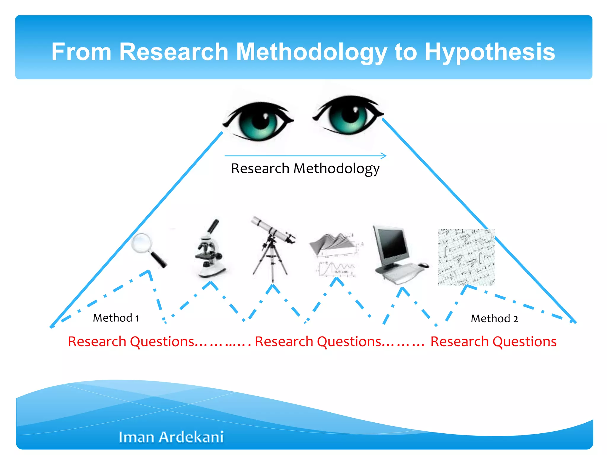
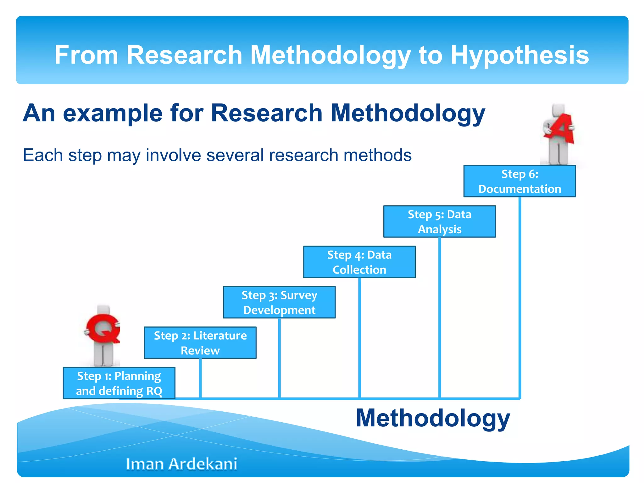
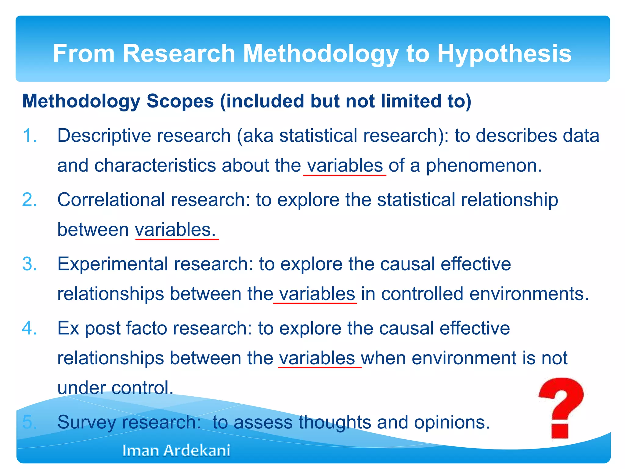
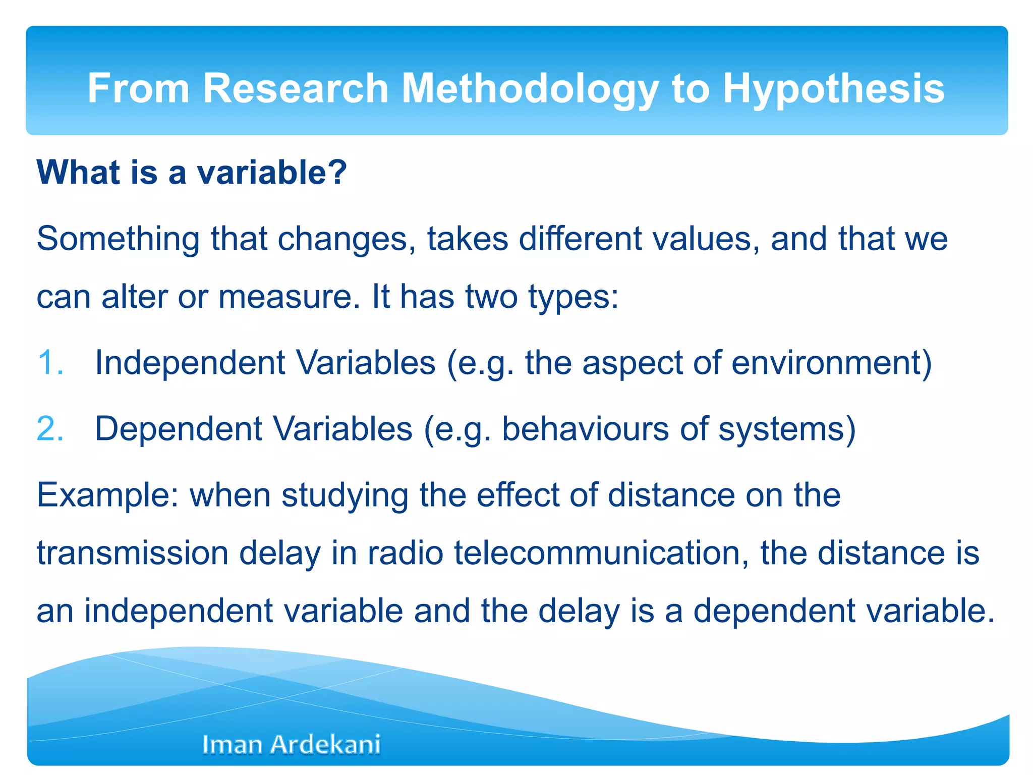
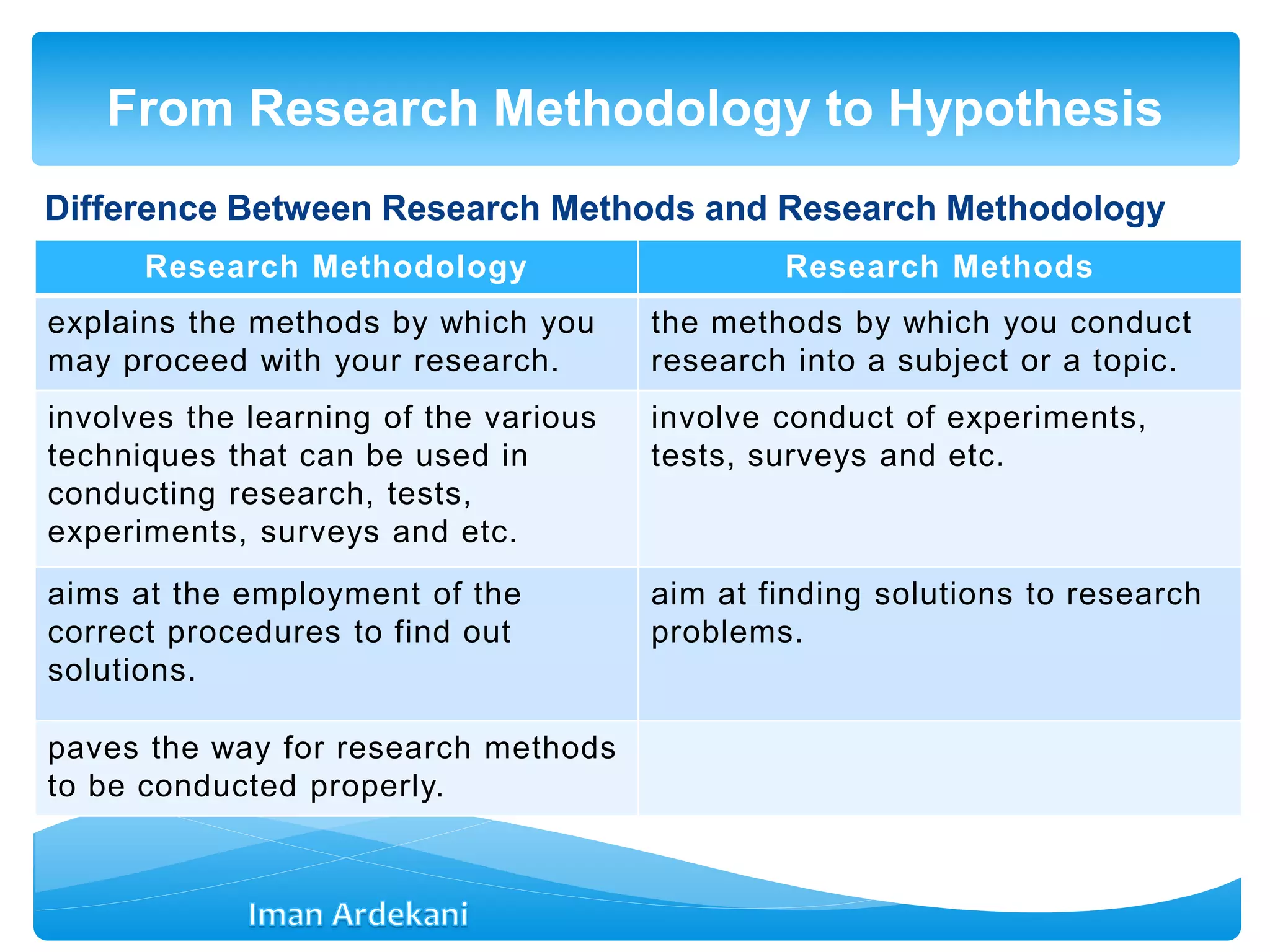
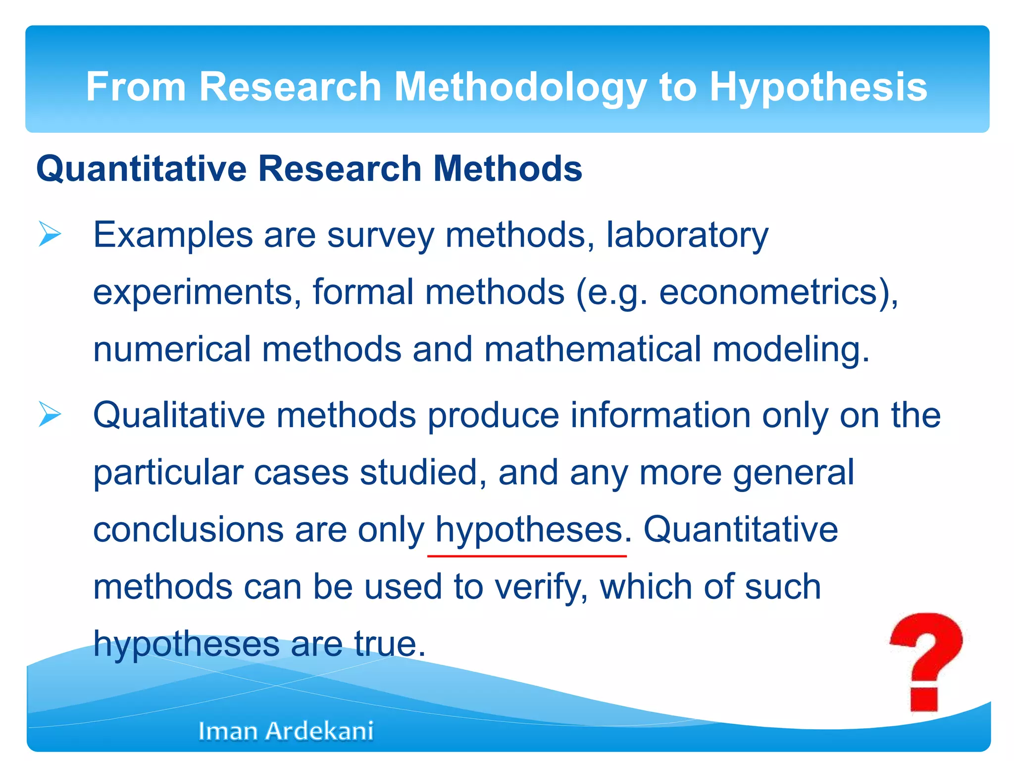
Discusses transitions from methodology to hypothesis involving steps, types, and definitions of research methods including qualitative and quantitative.
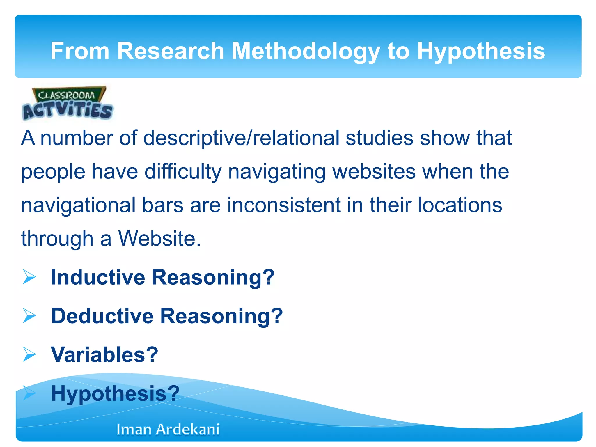
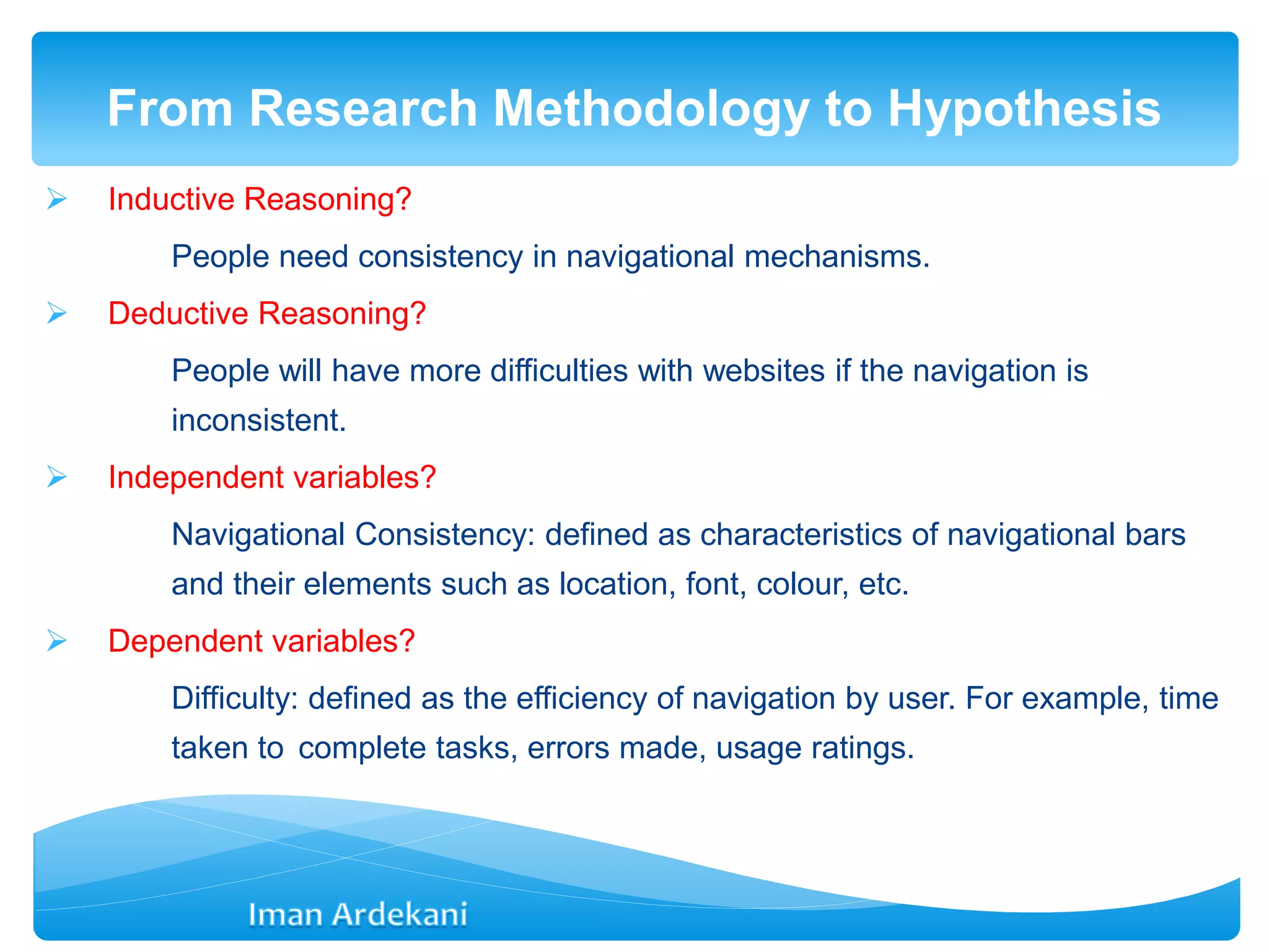
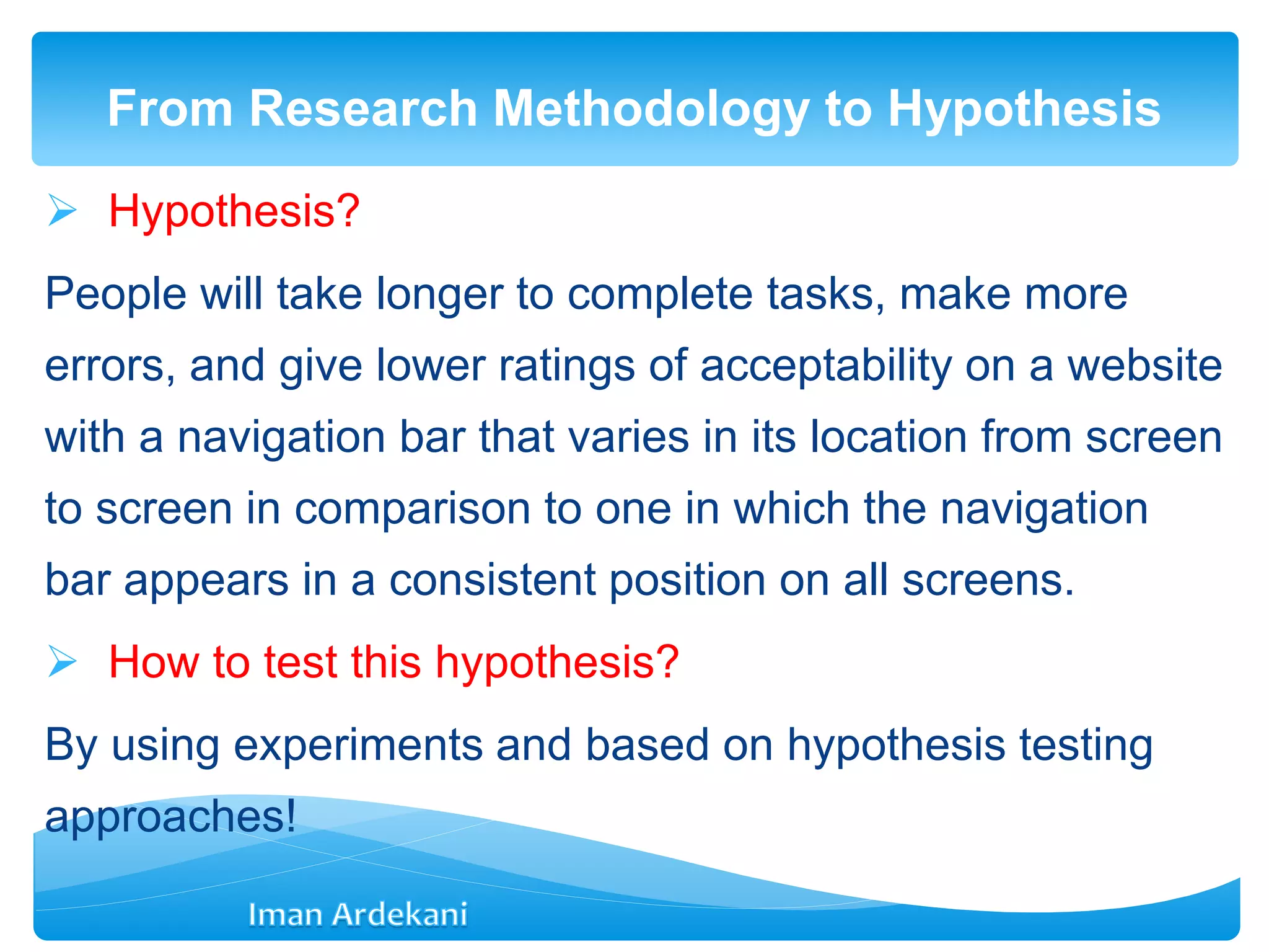
Details the hypothesis formulation process through examples and methods to test hypotheses.
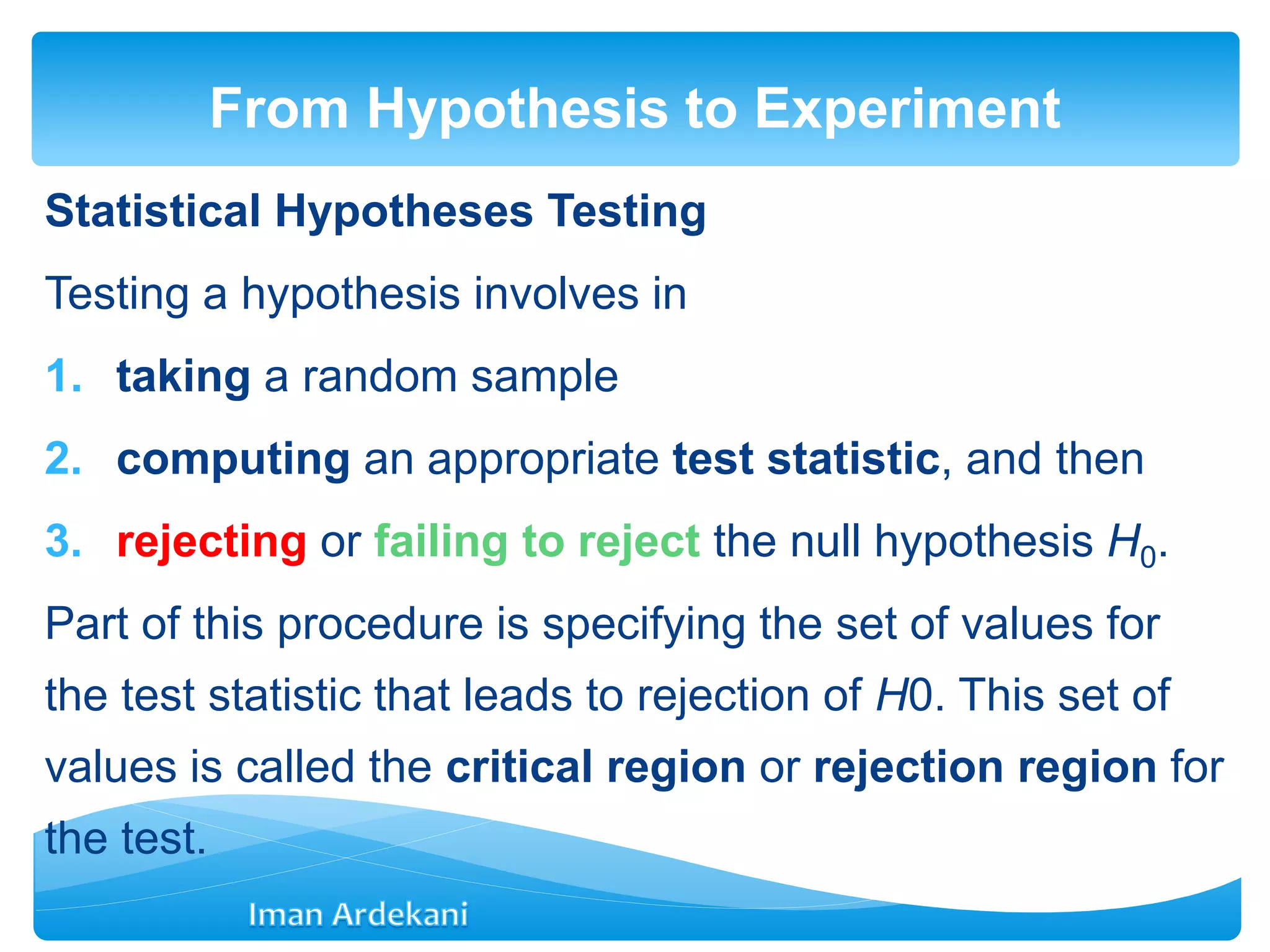
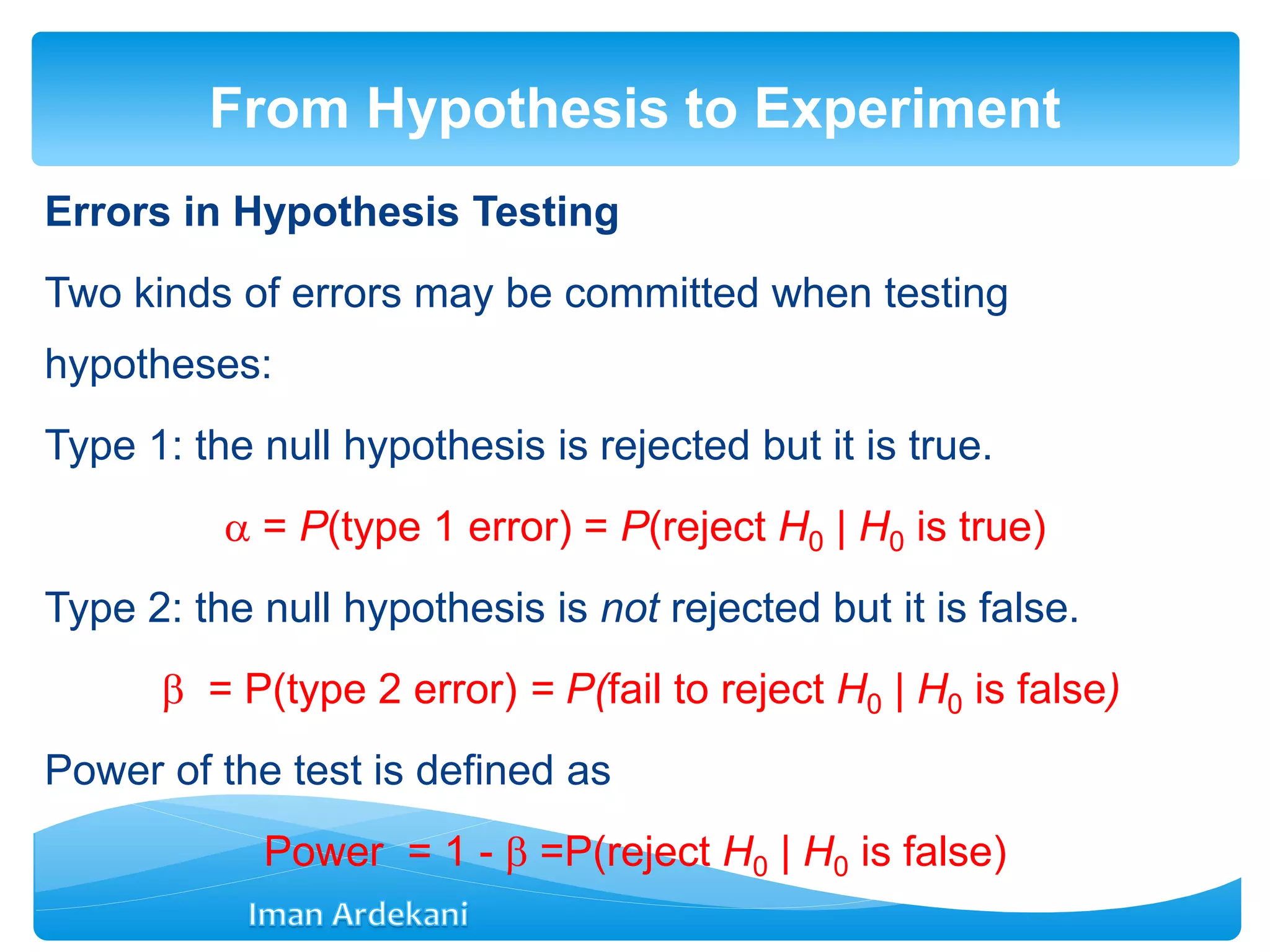
Describes statistical hypothesis testing along with Type 1 and Type 2 errors, significance levels, and the power of tests.
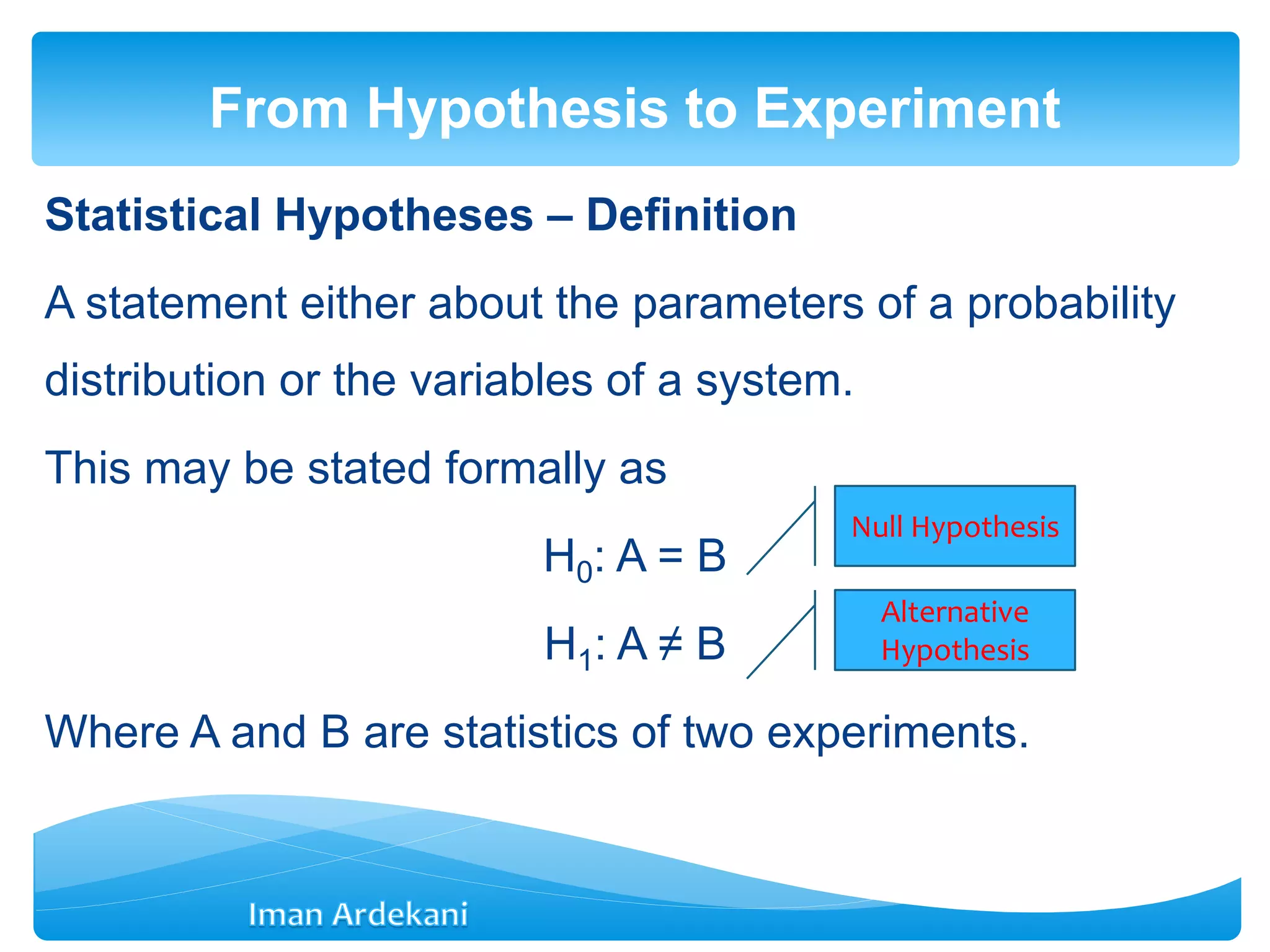
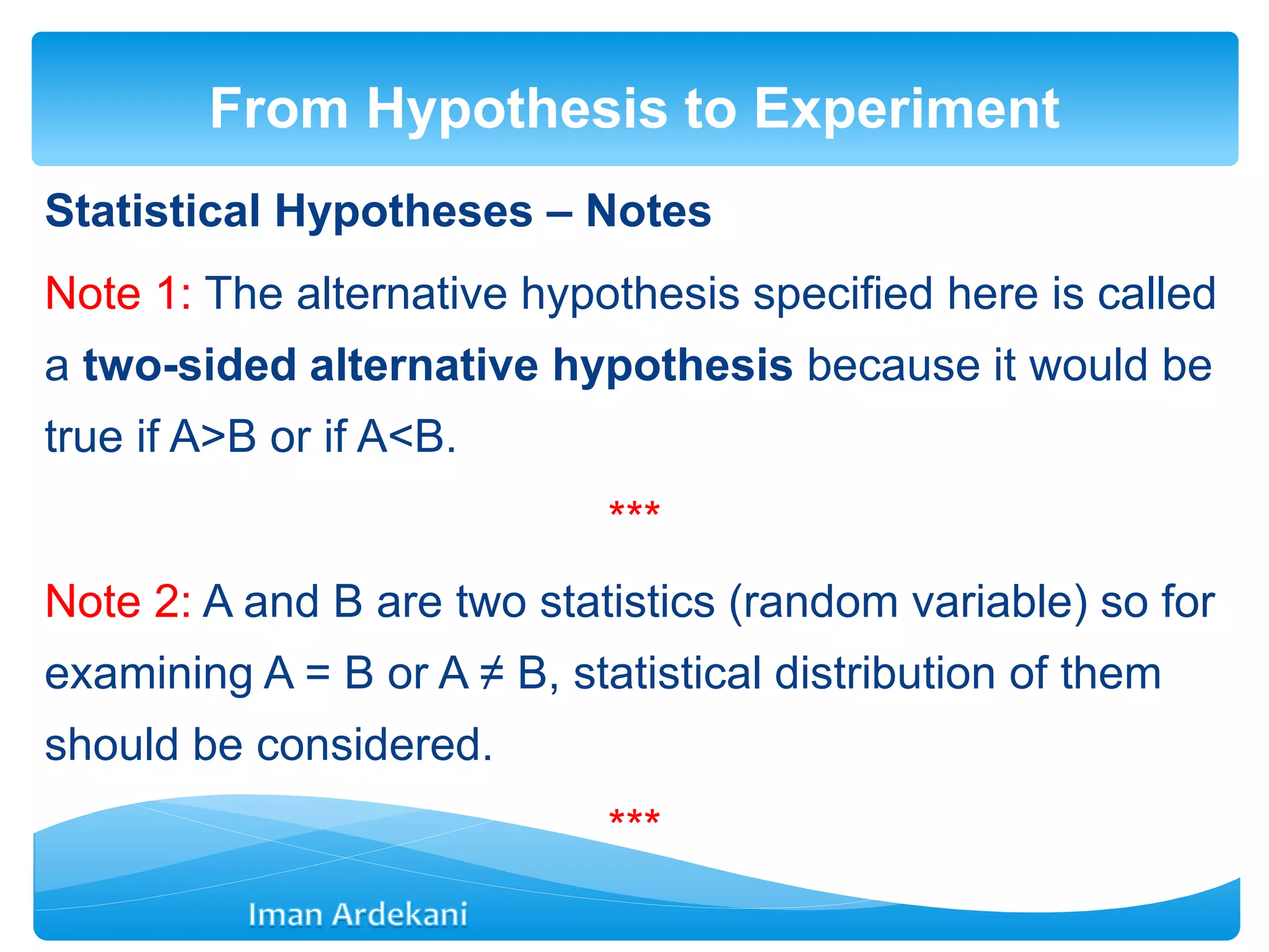
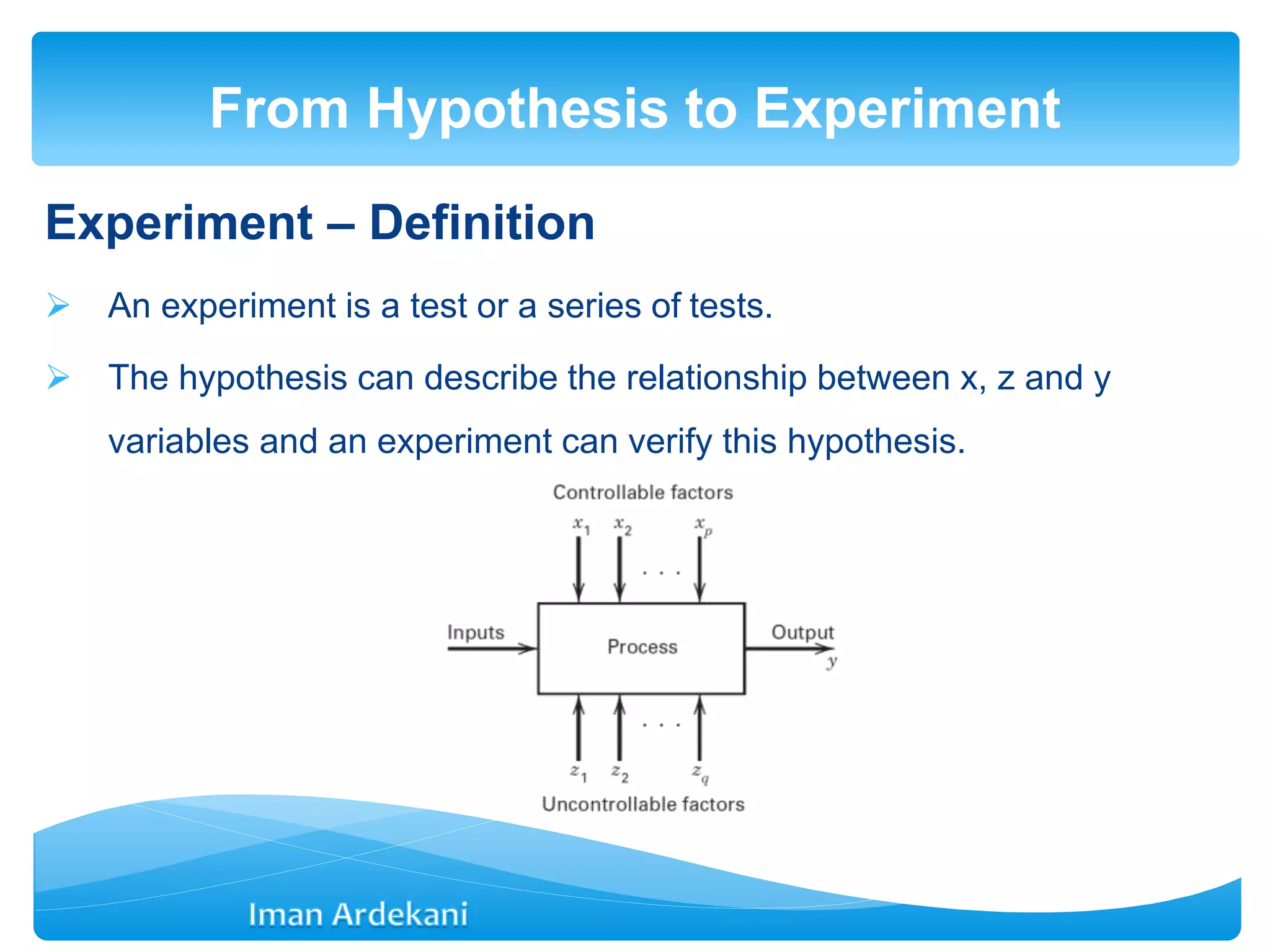
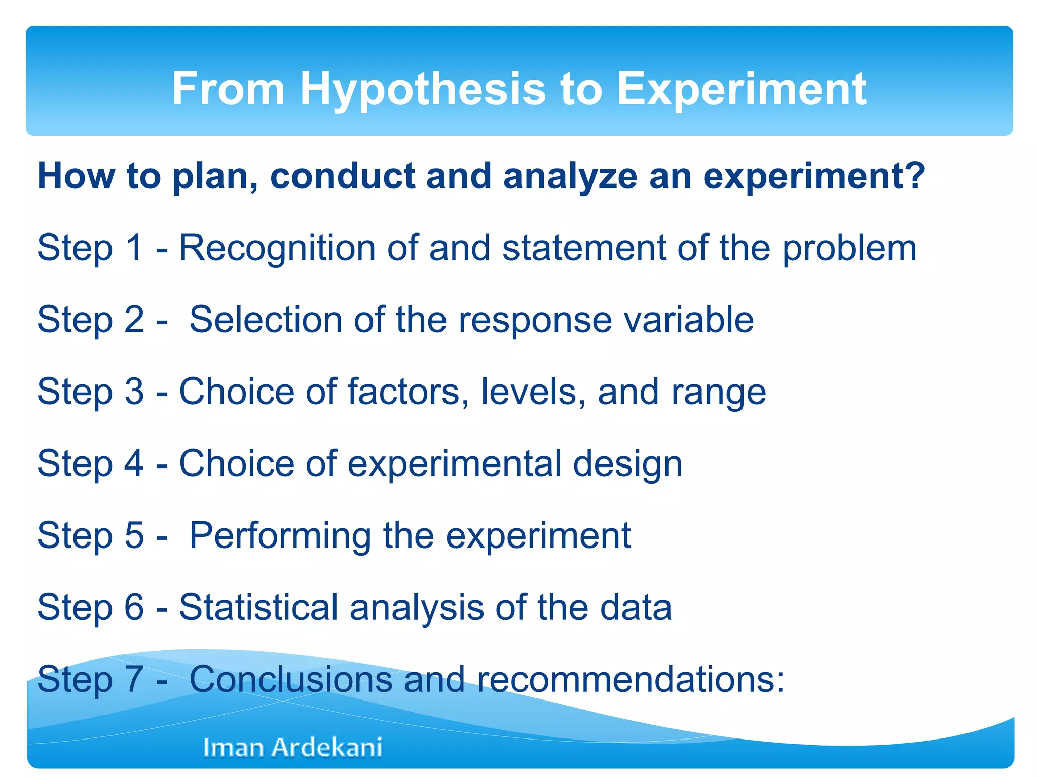
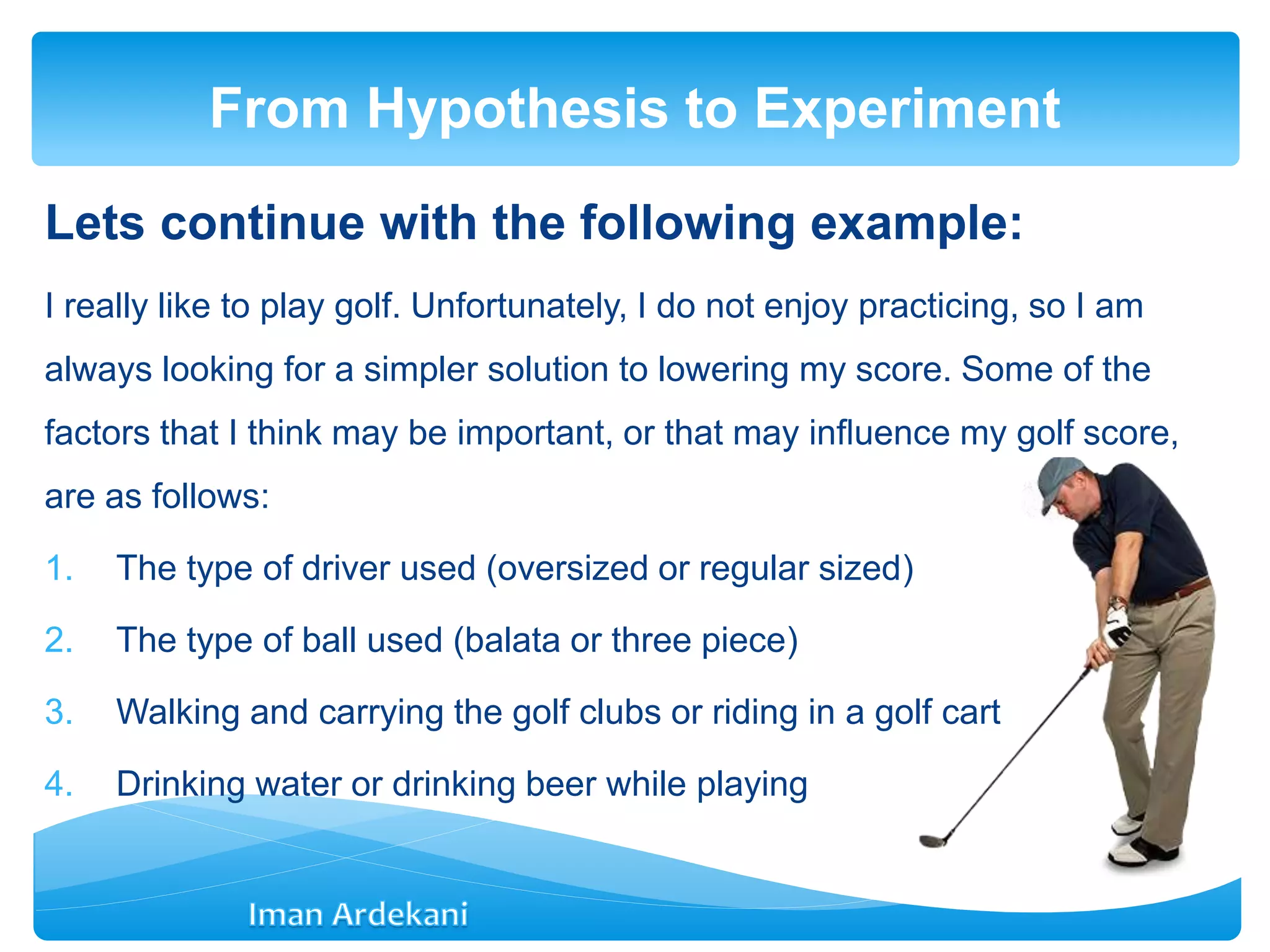
Defines statistical hypotheses, discusses experimental designs, and outlines planning stages for conducting experiments.
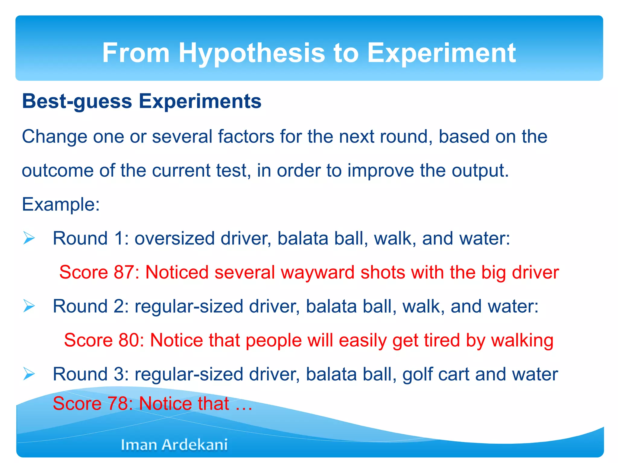
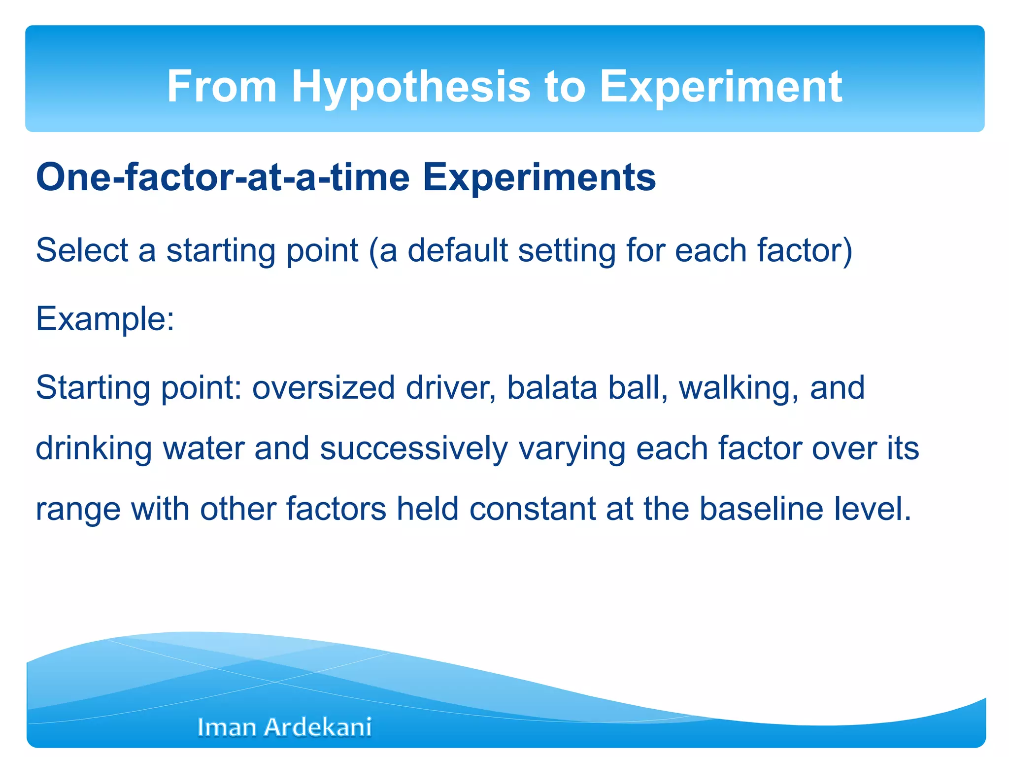
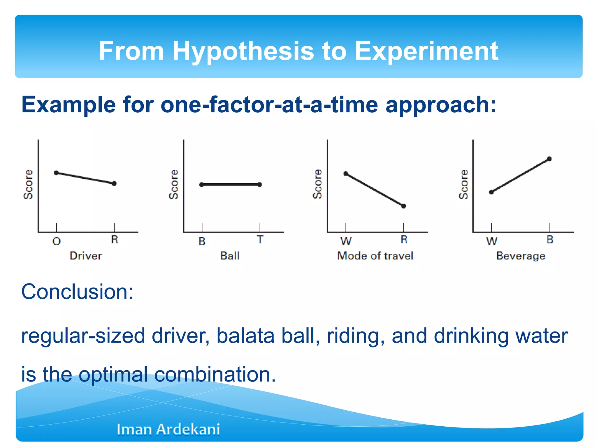
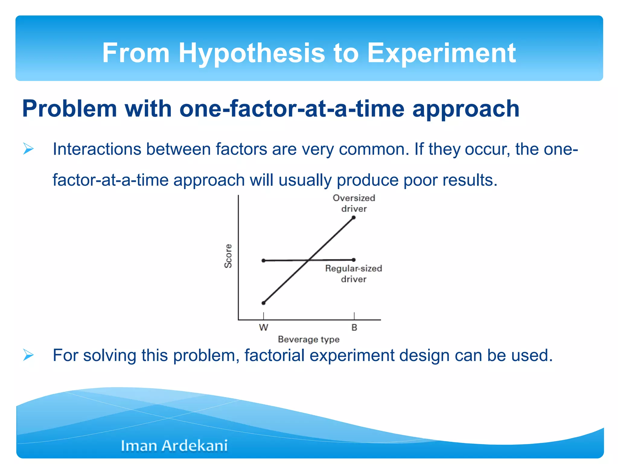
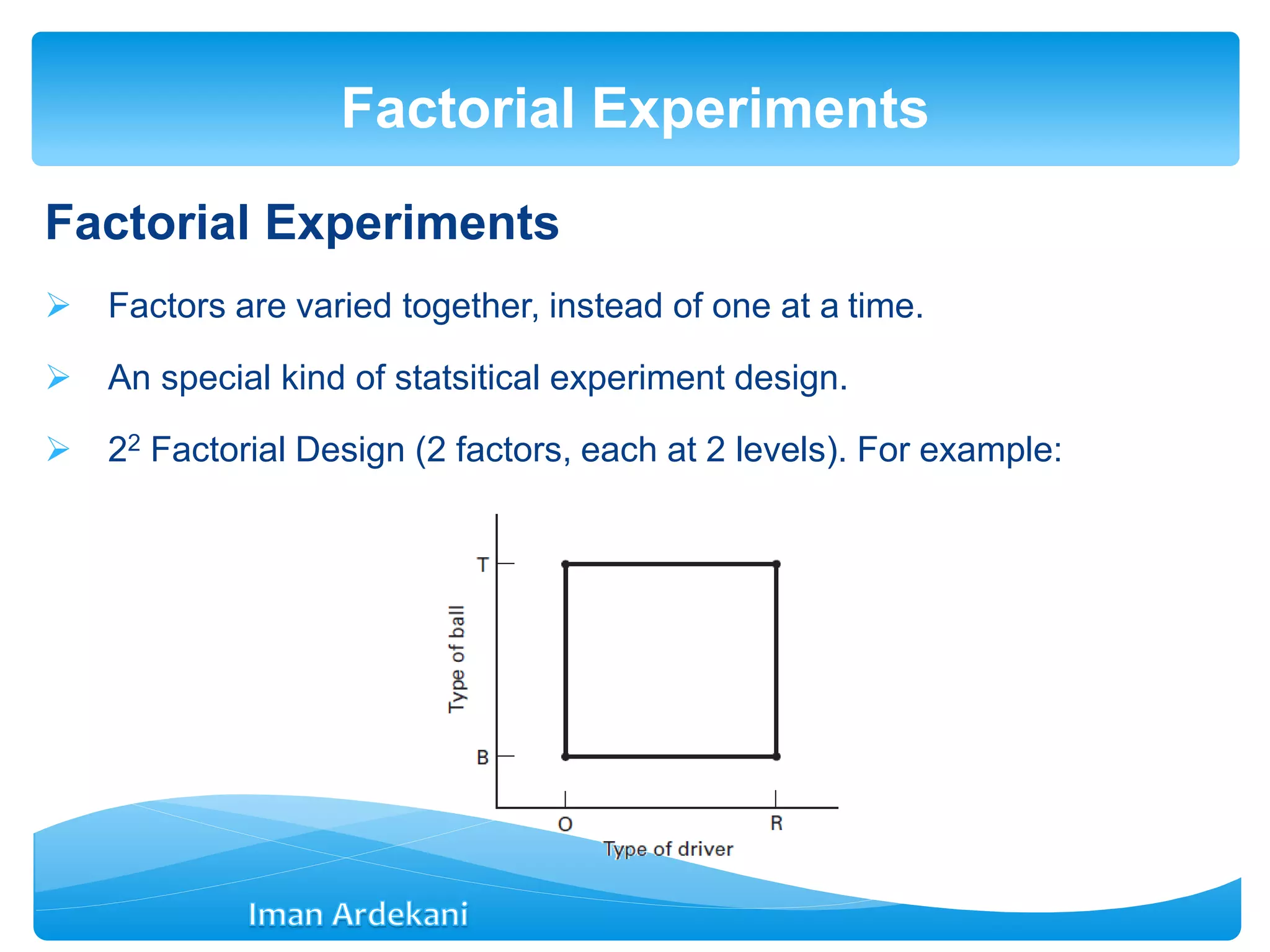
Explains best-guess experiments and issues with one-factor-at-a-time approaches, introducing factorial experiments as an alternative.
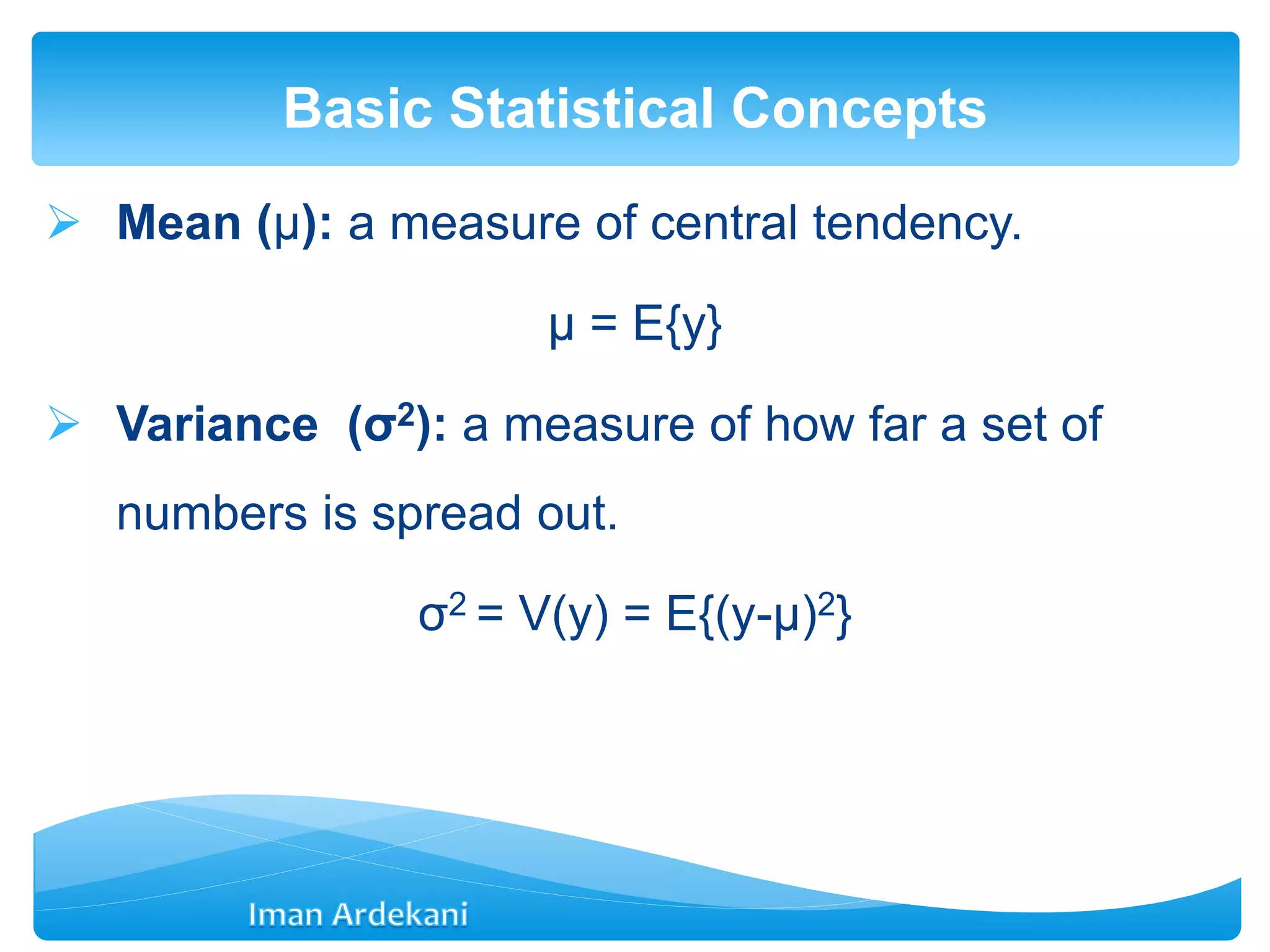
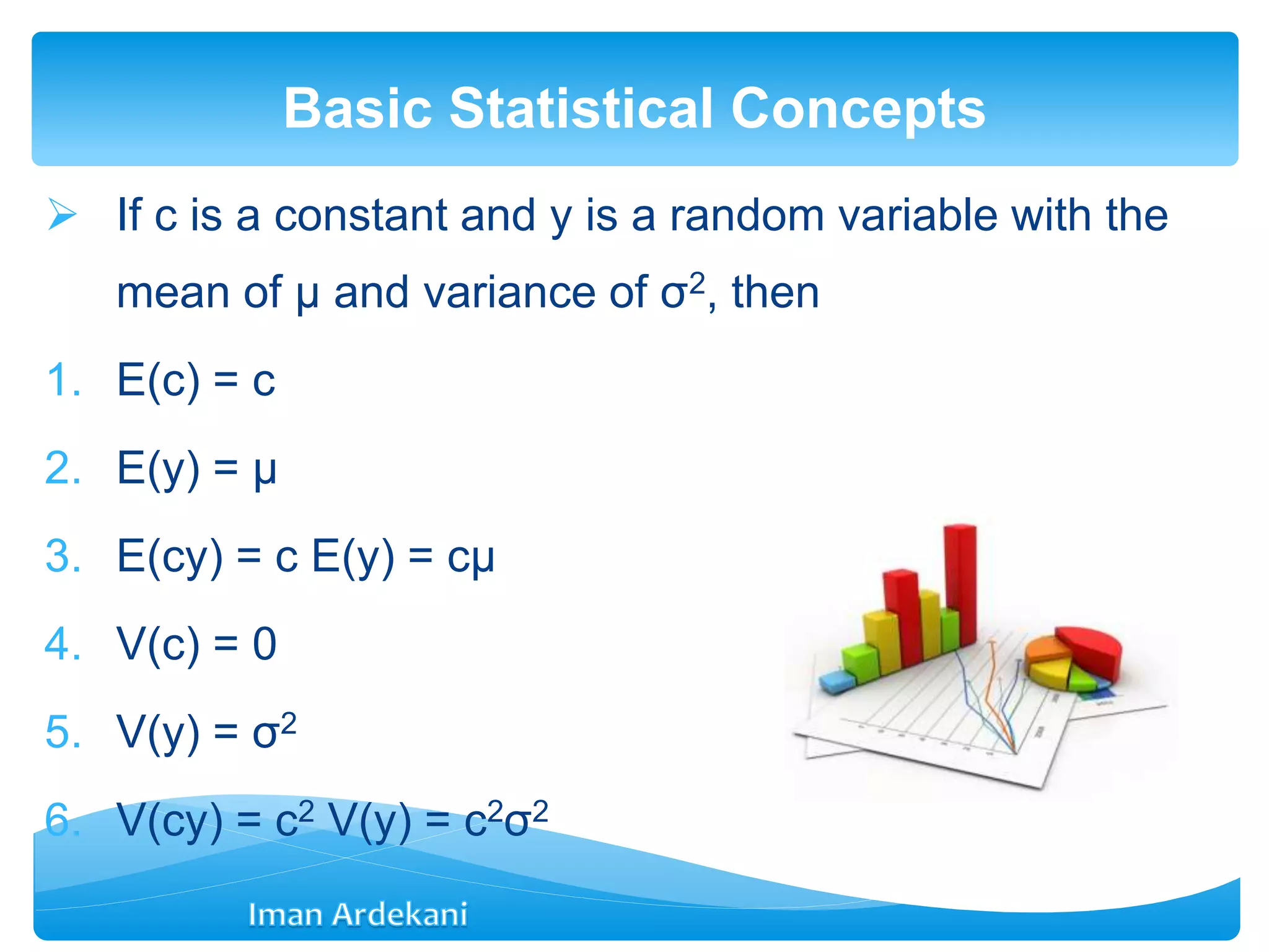
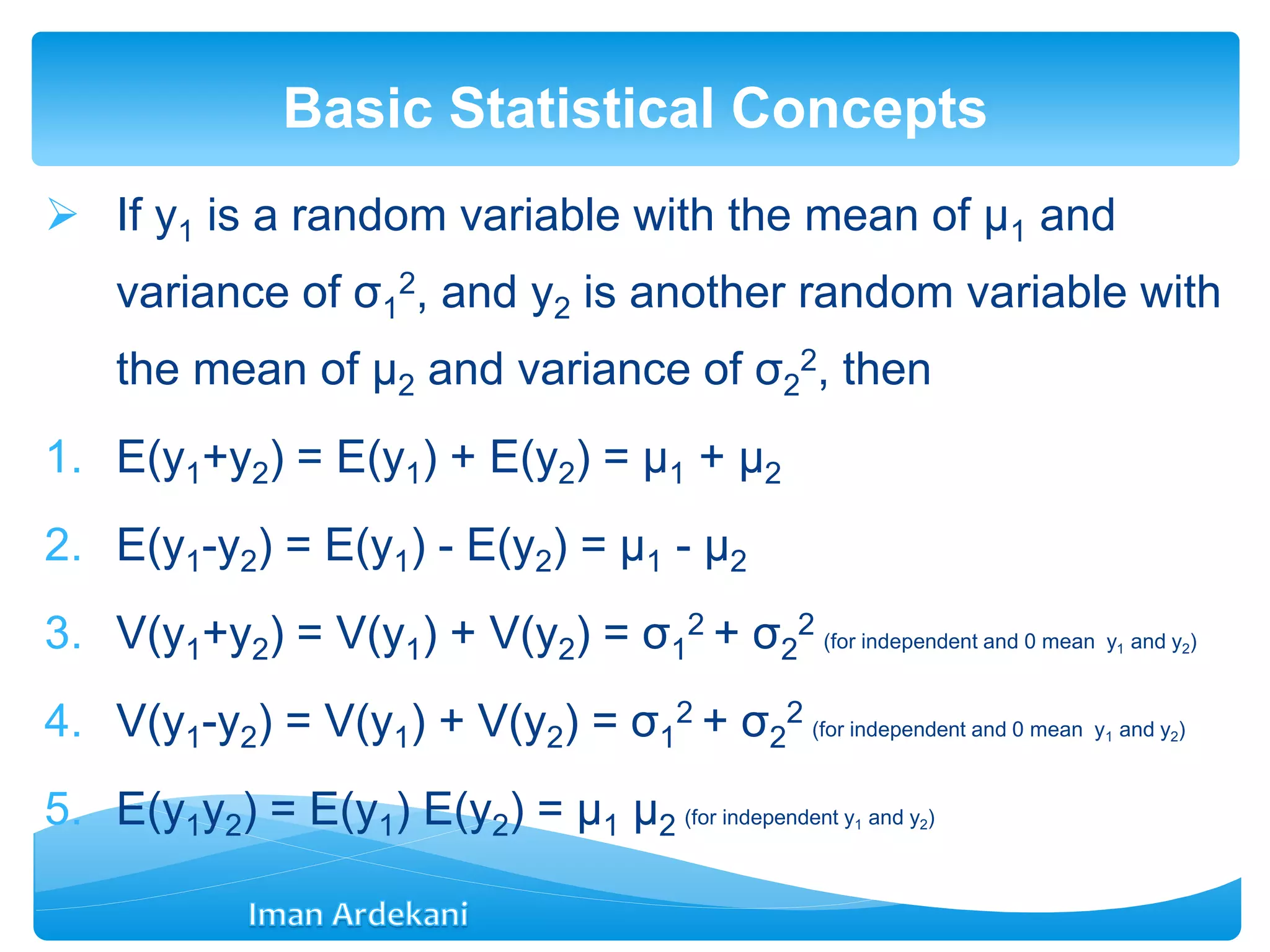
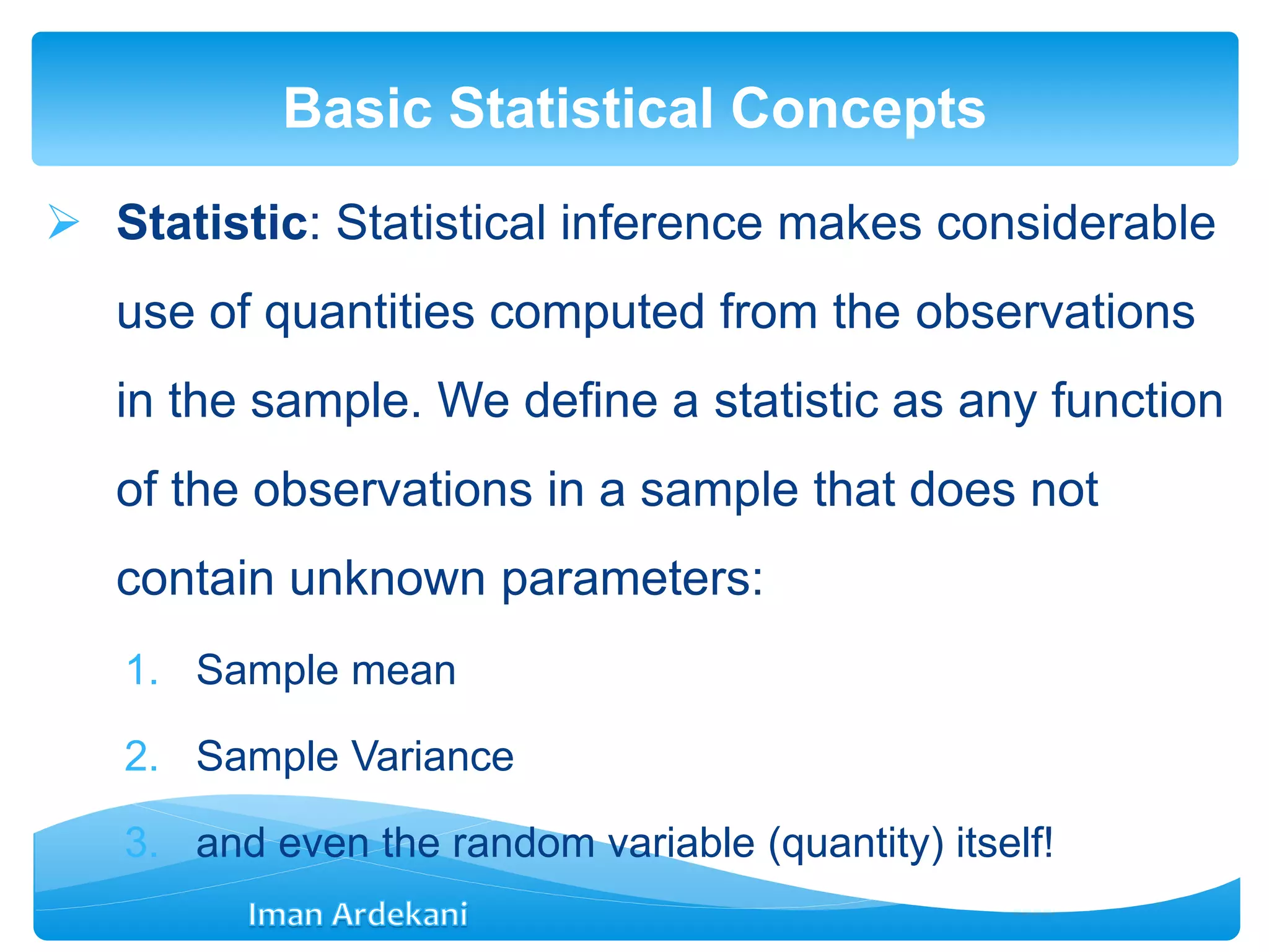
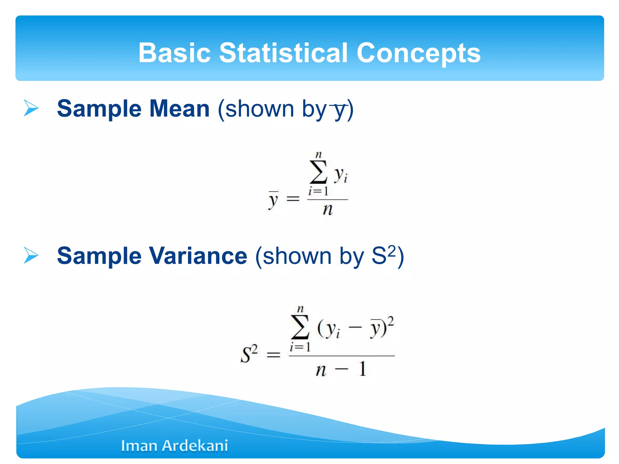
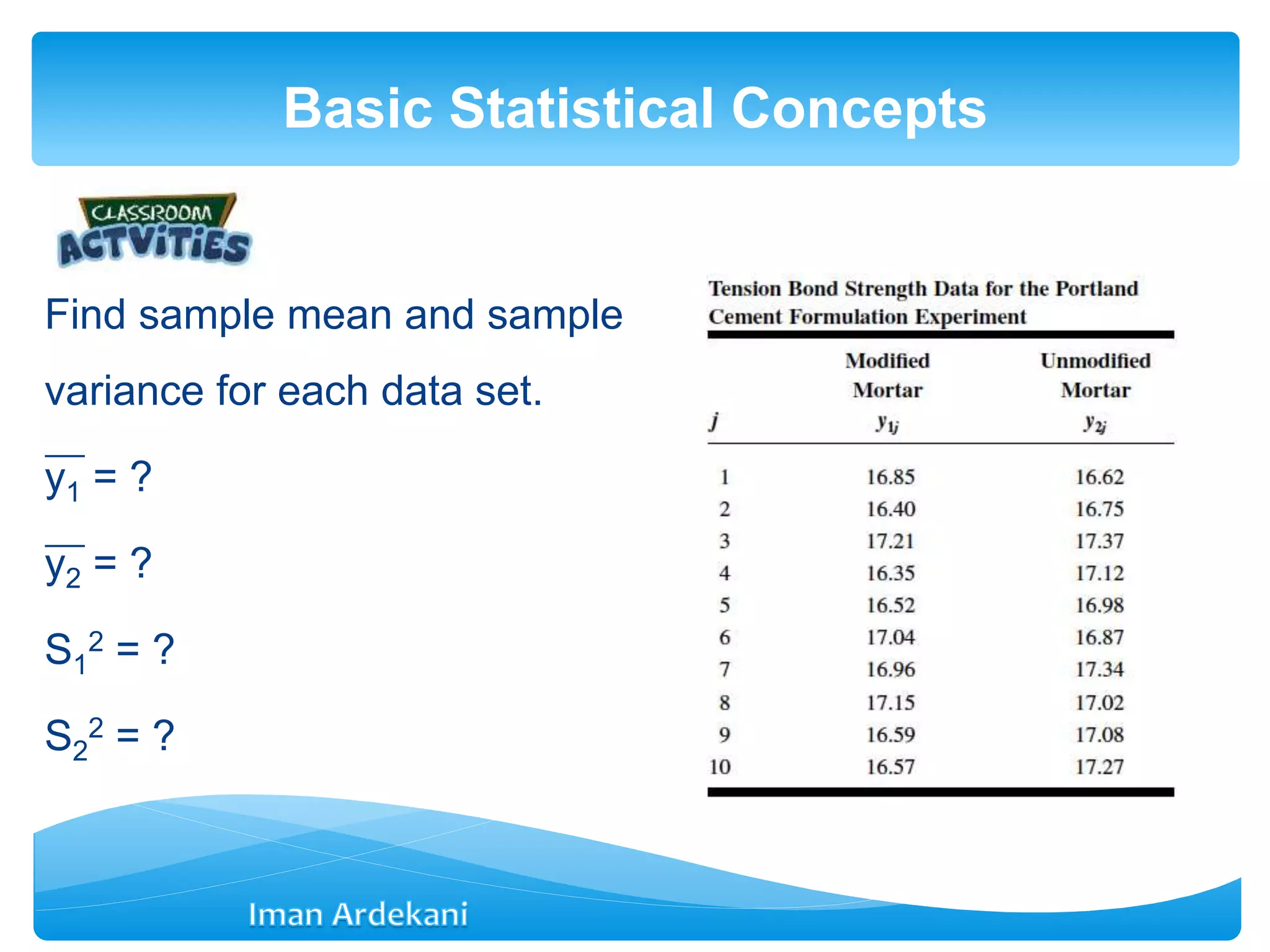
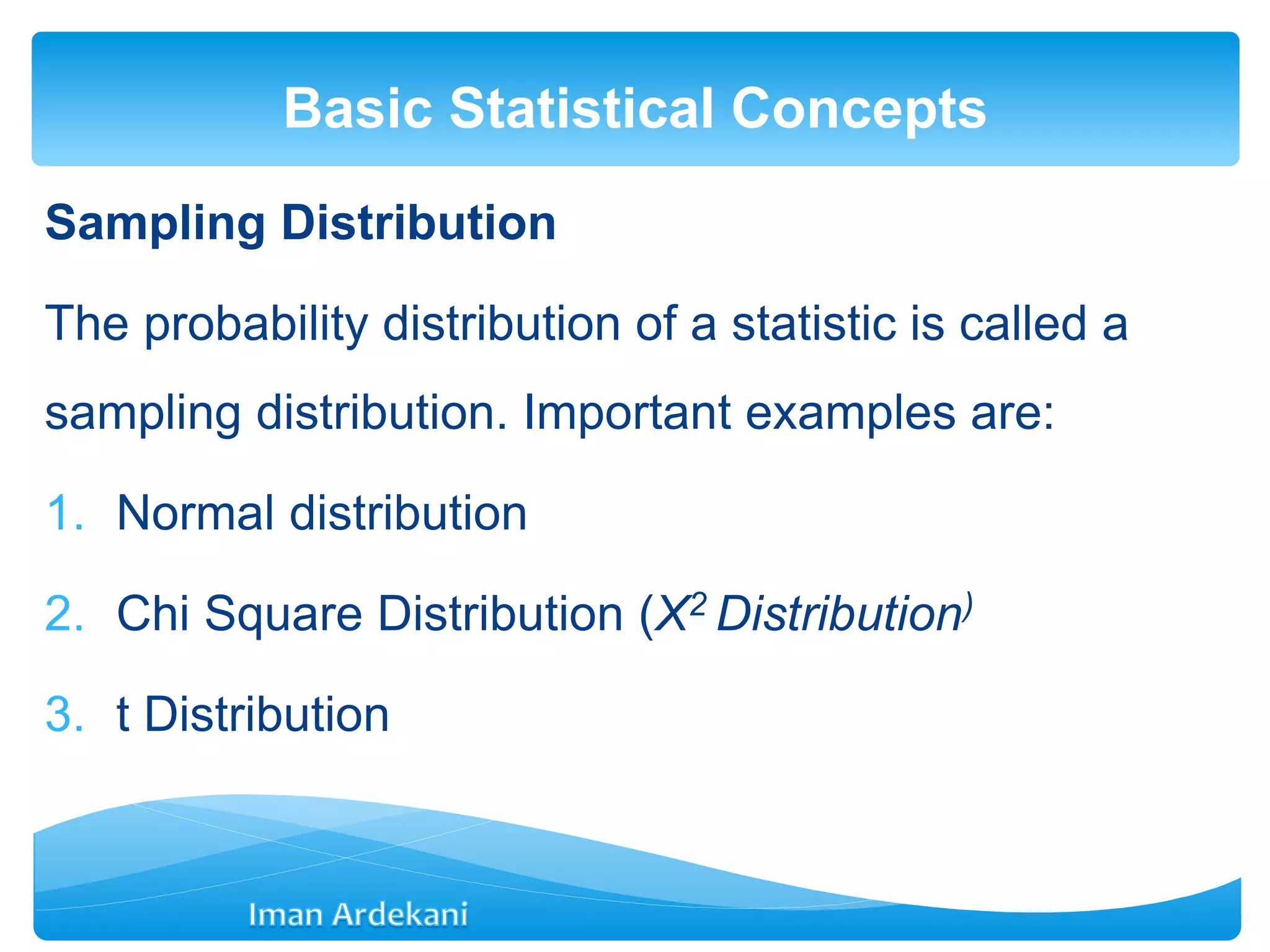
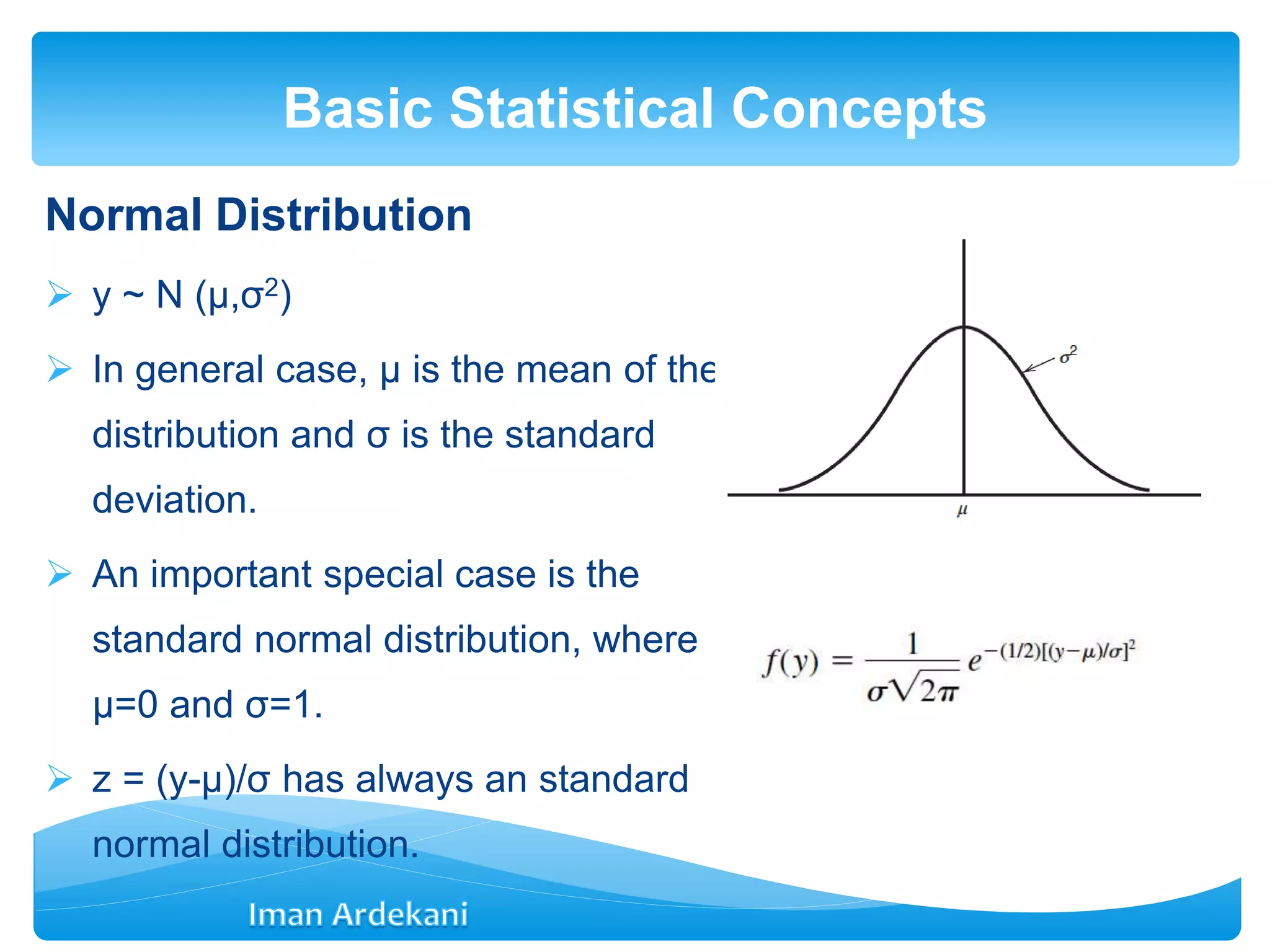
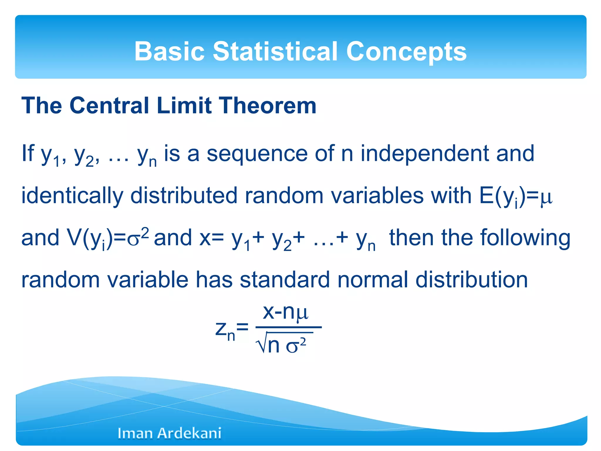
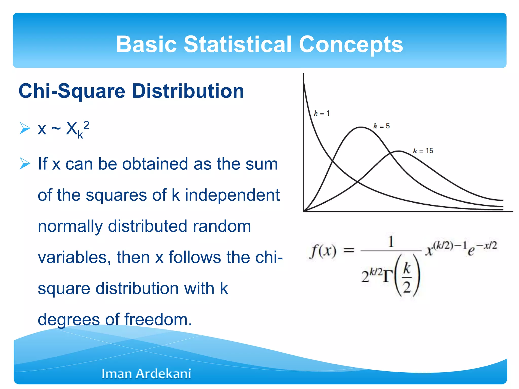
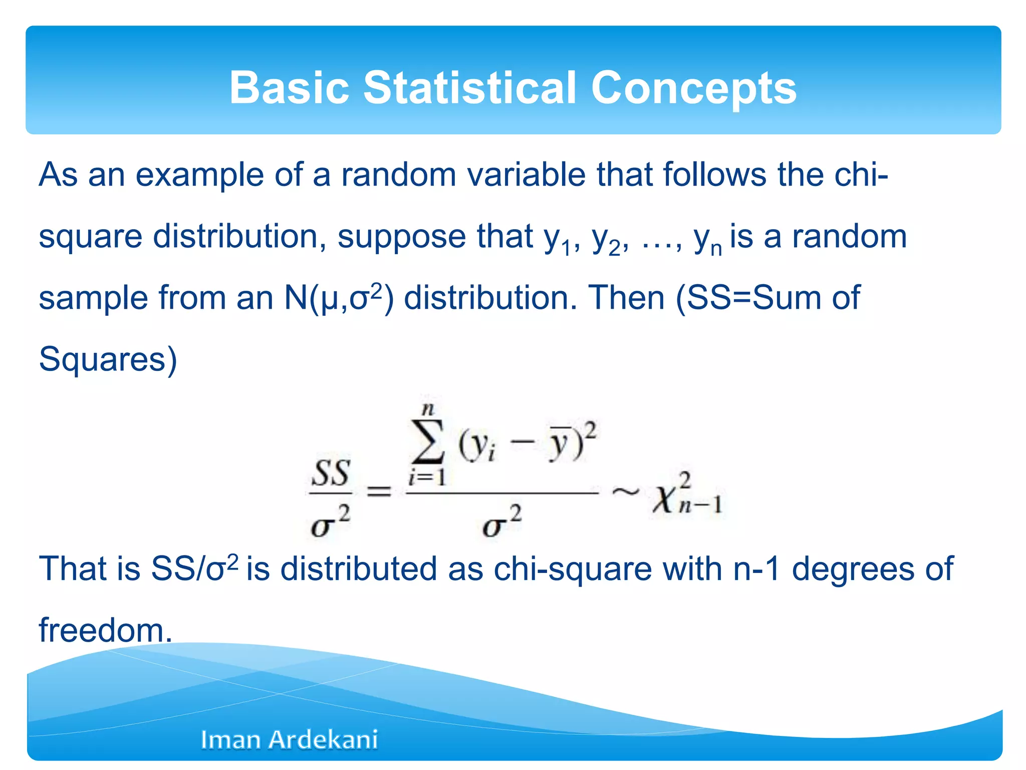
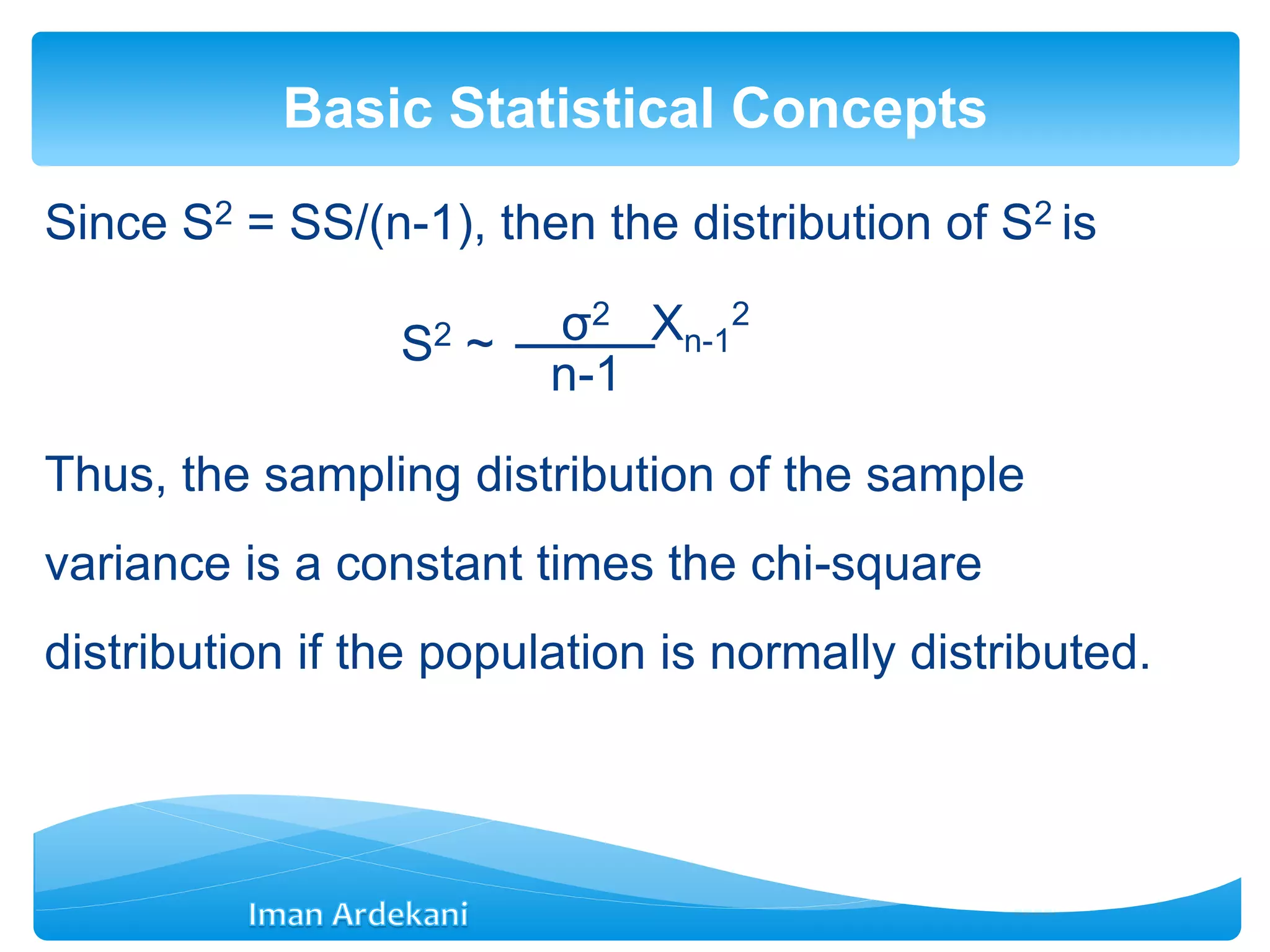
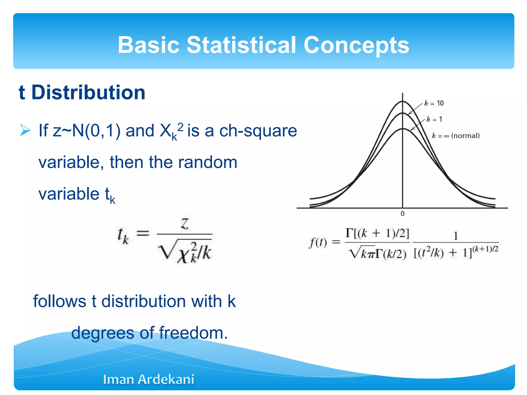
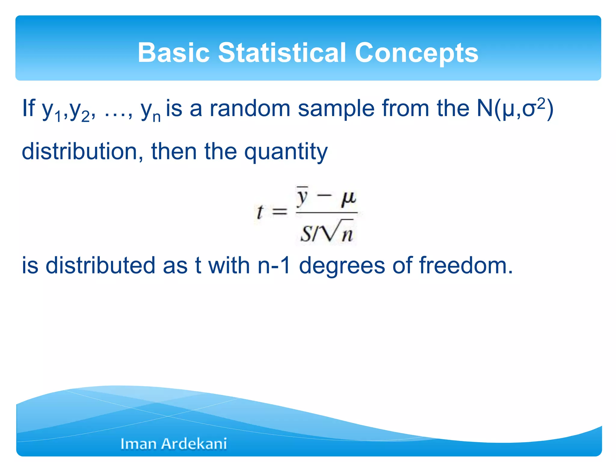
Introduces statistical concepts including mean, variance, sampling distributions, and various distributions utilized in statistics.
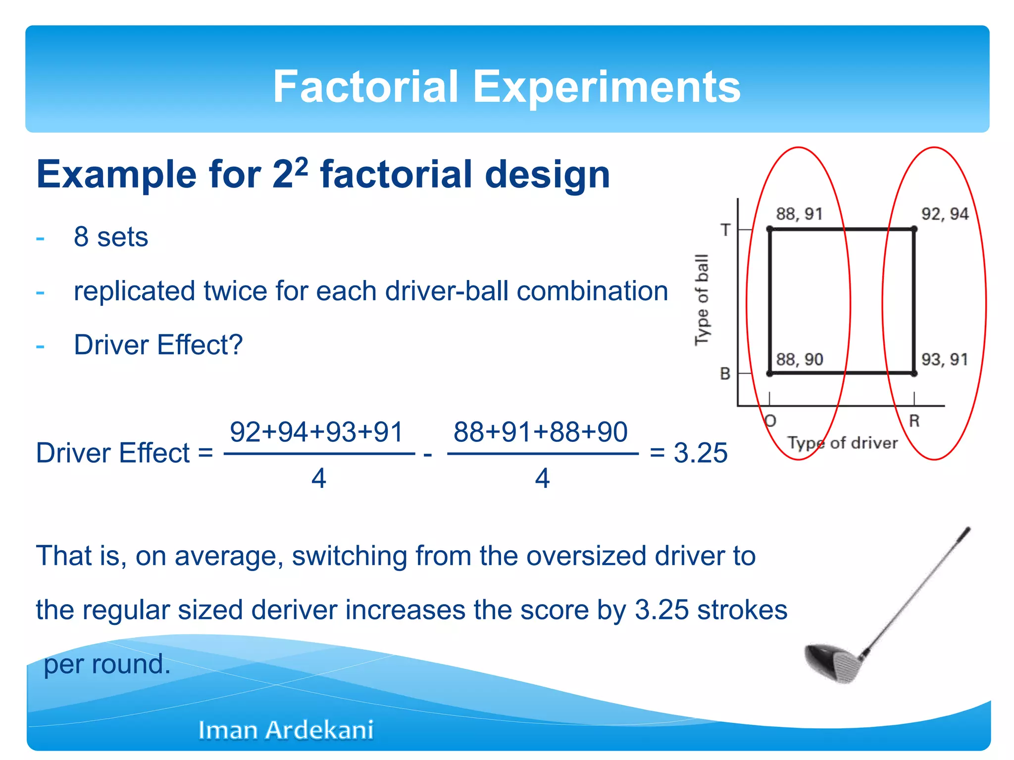
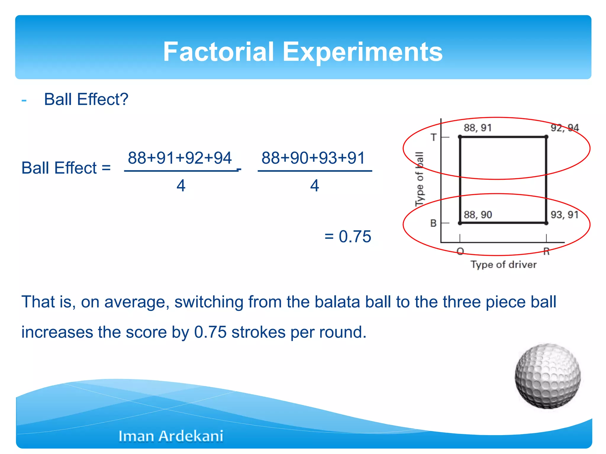
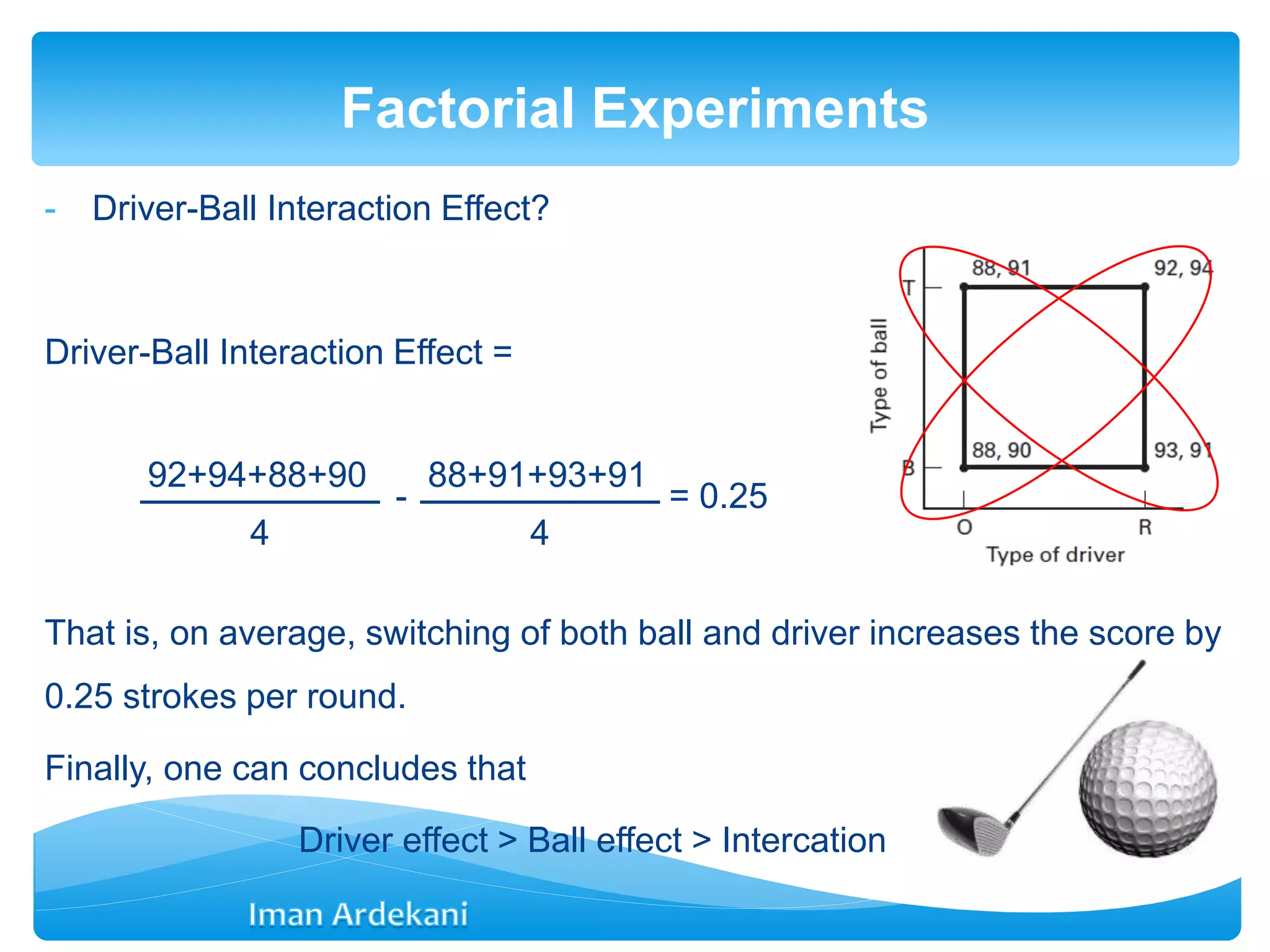
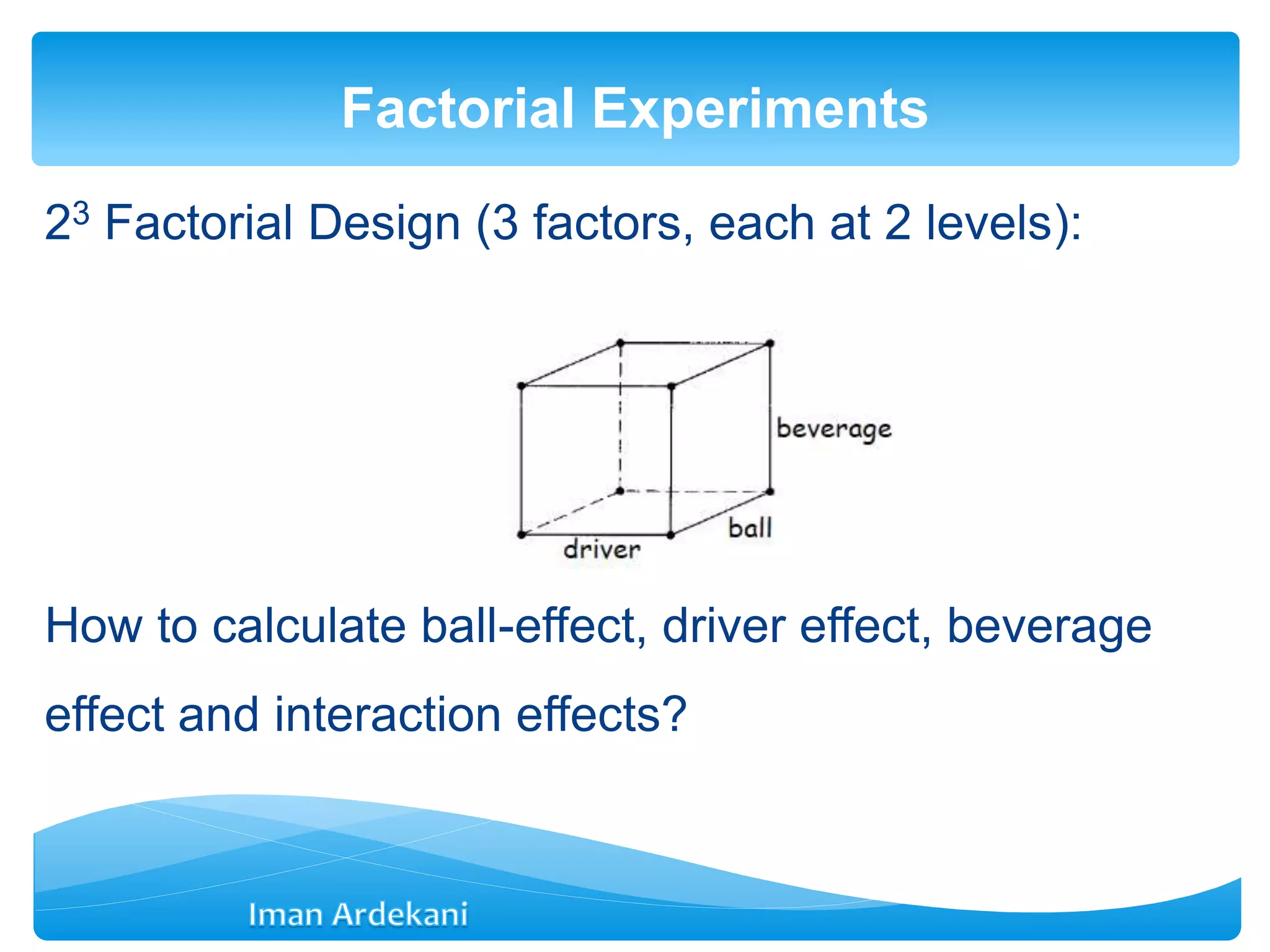
Defines factorial experiment designs, examples of 2^2 and 3^2 designs, and their applications.
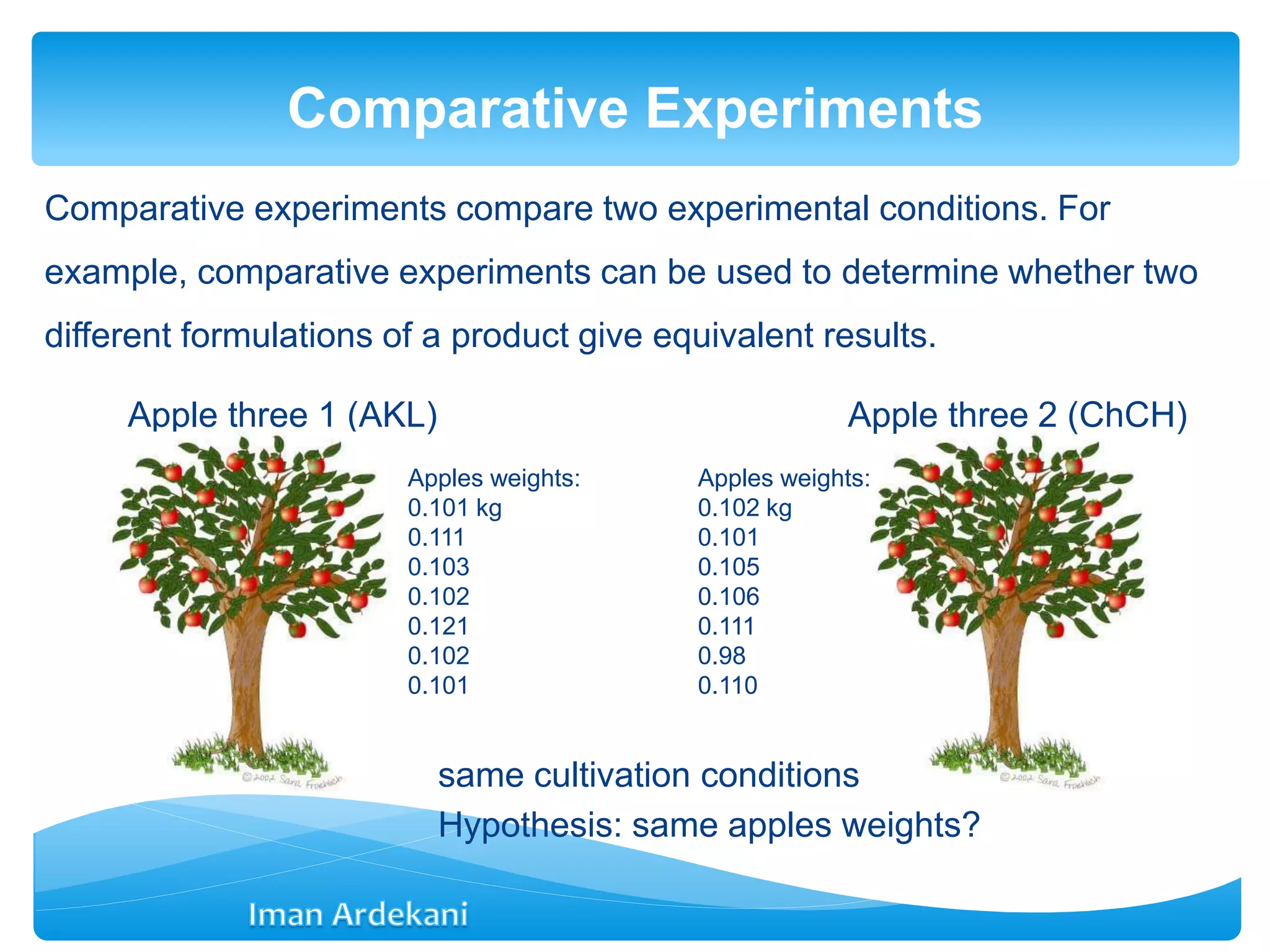
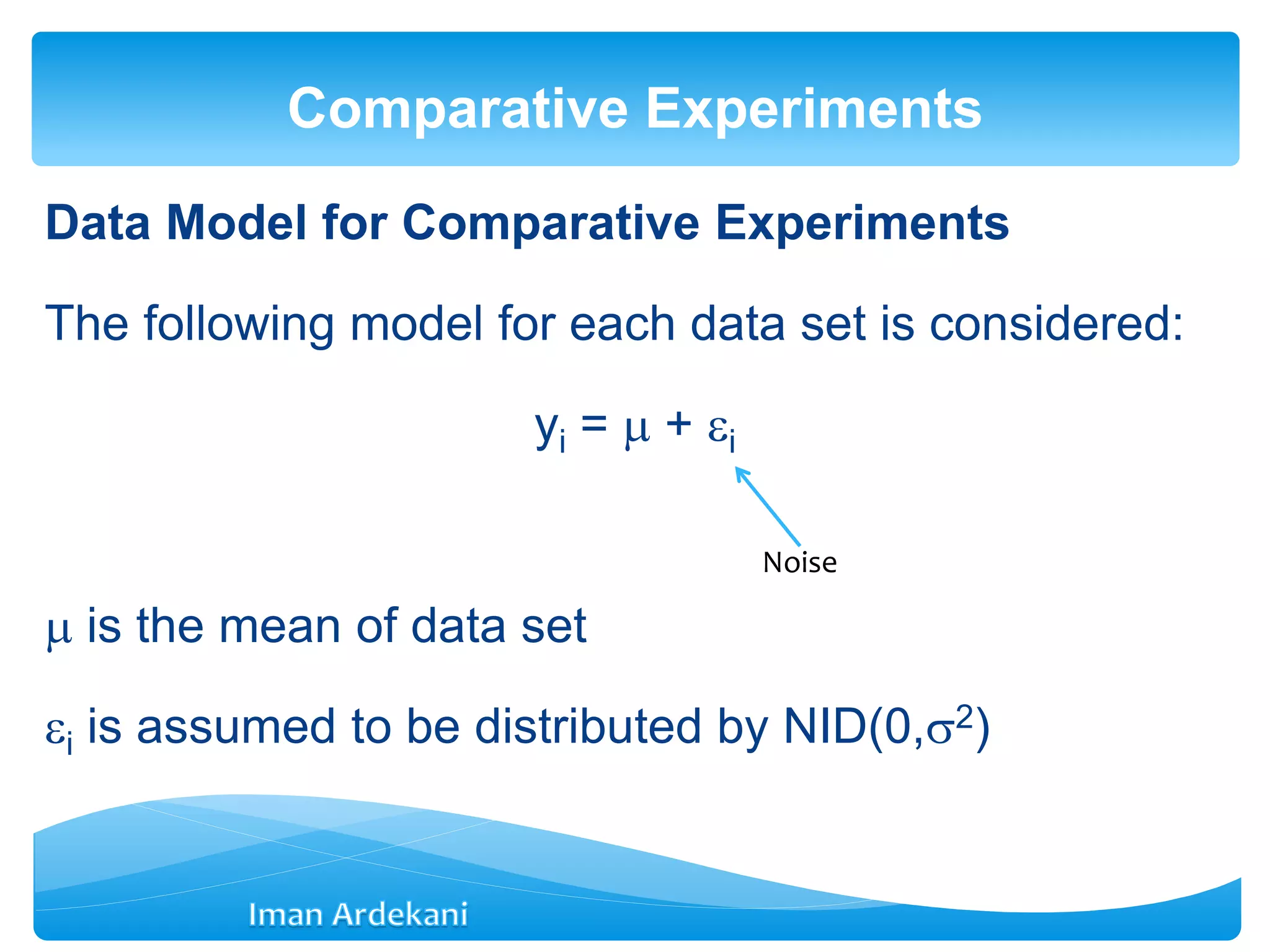
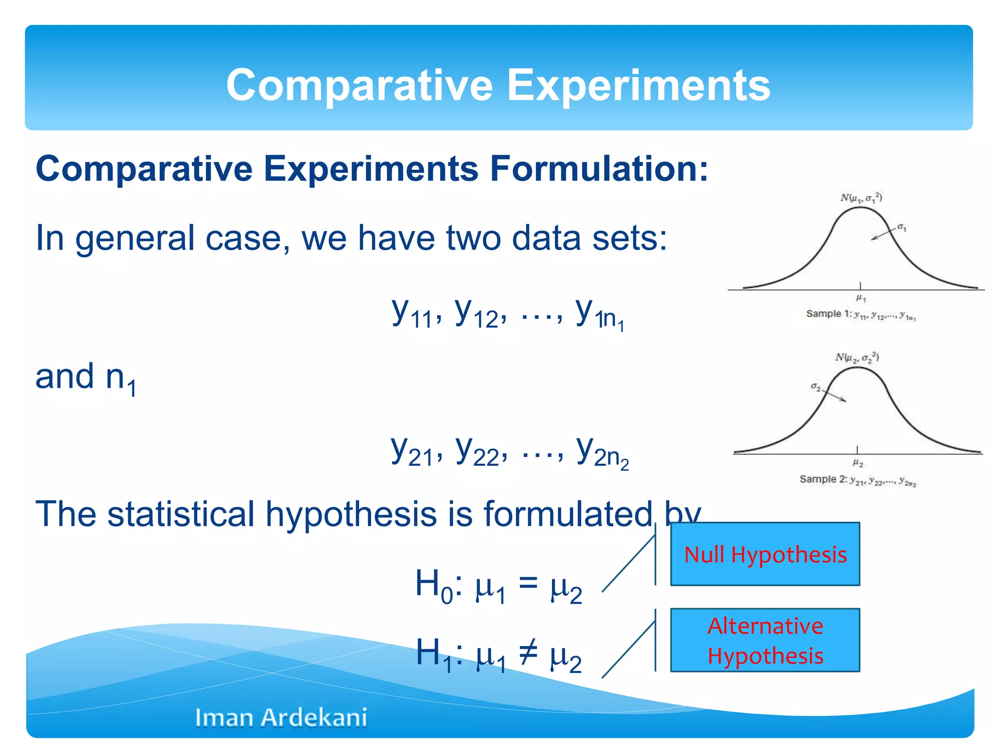
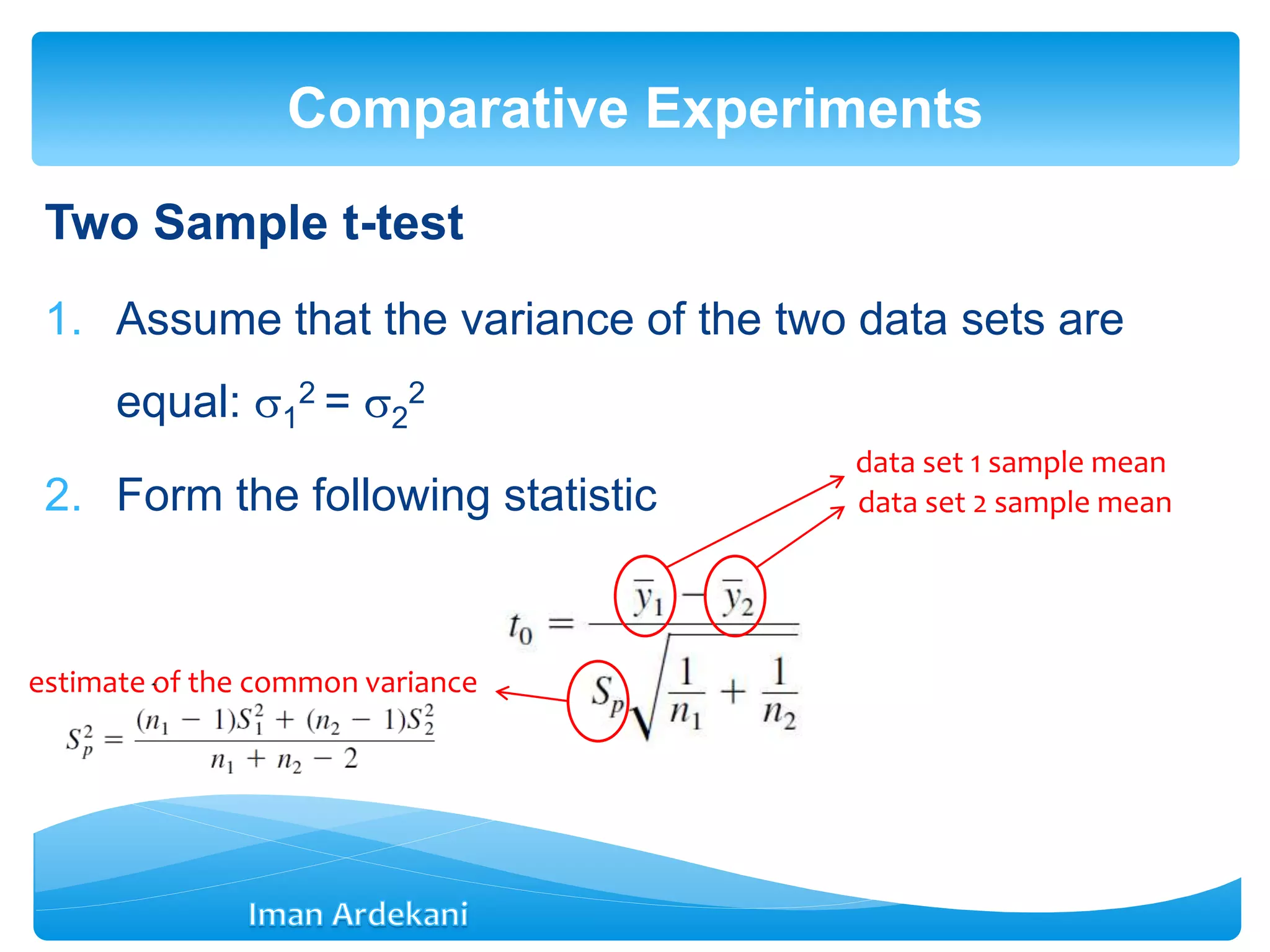
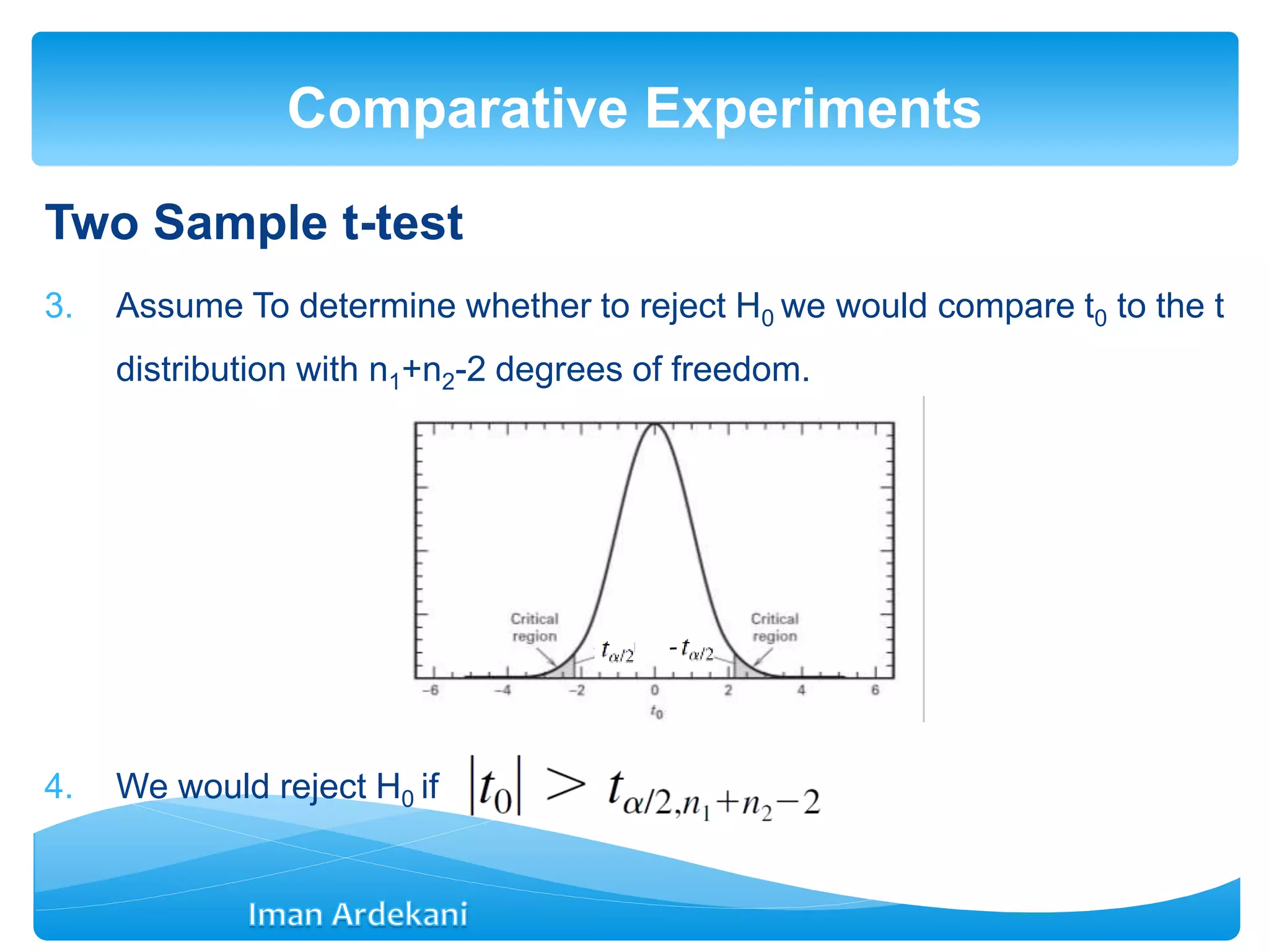
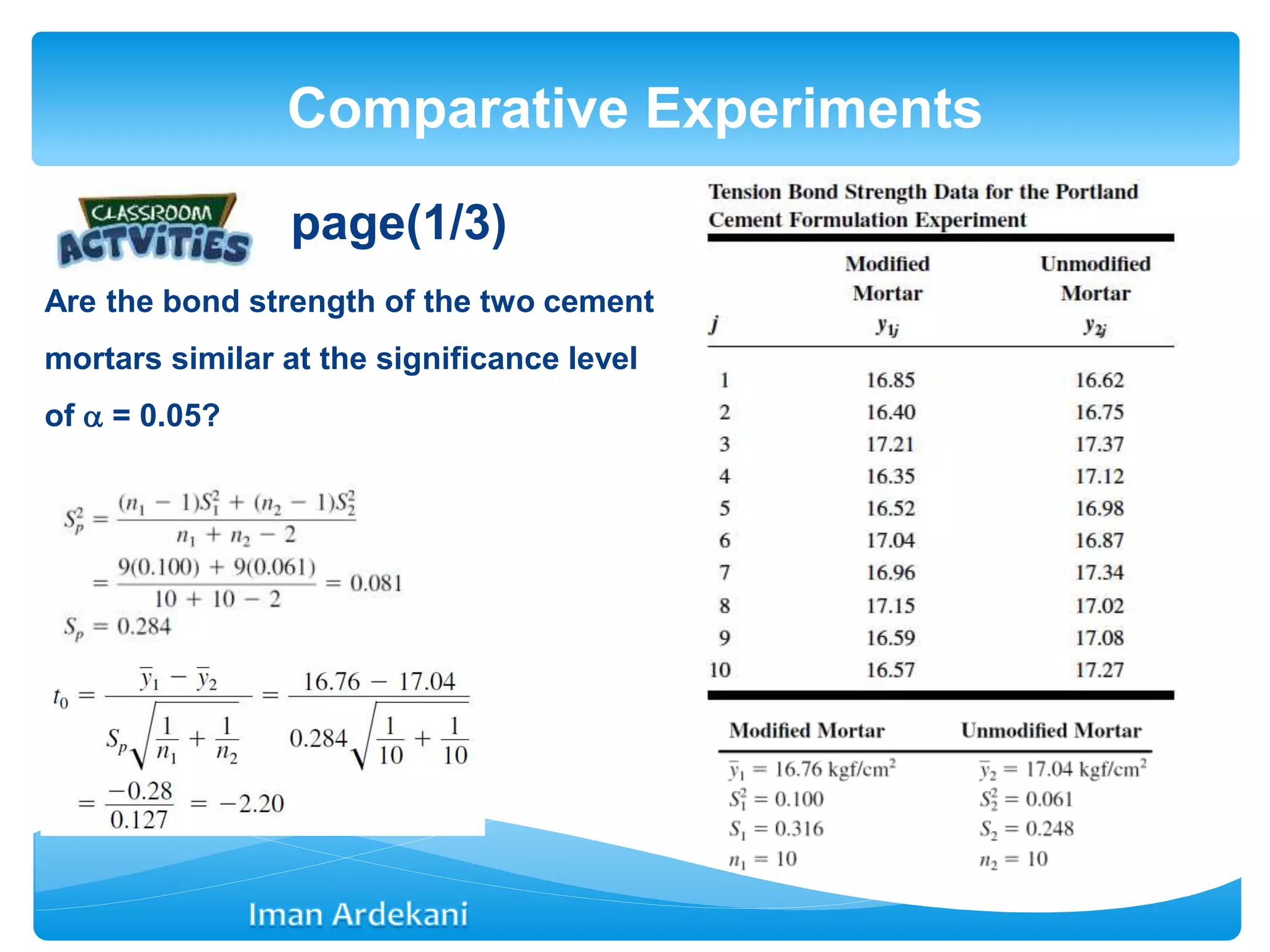
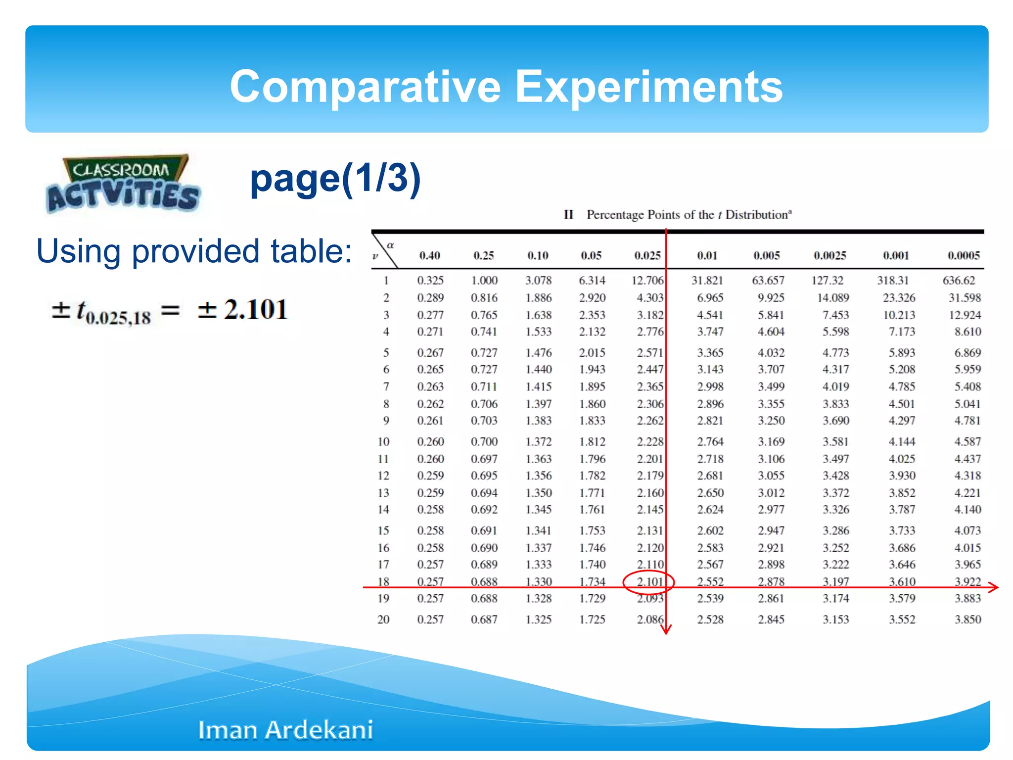
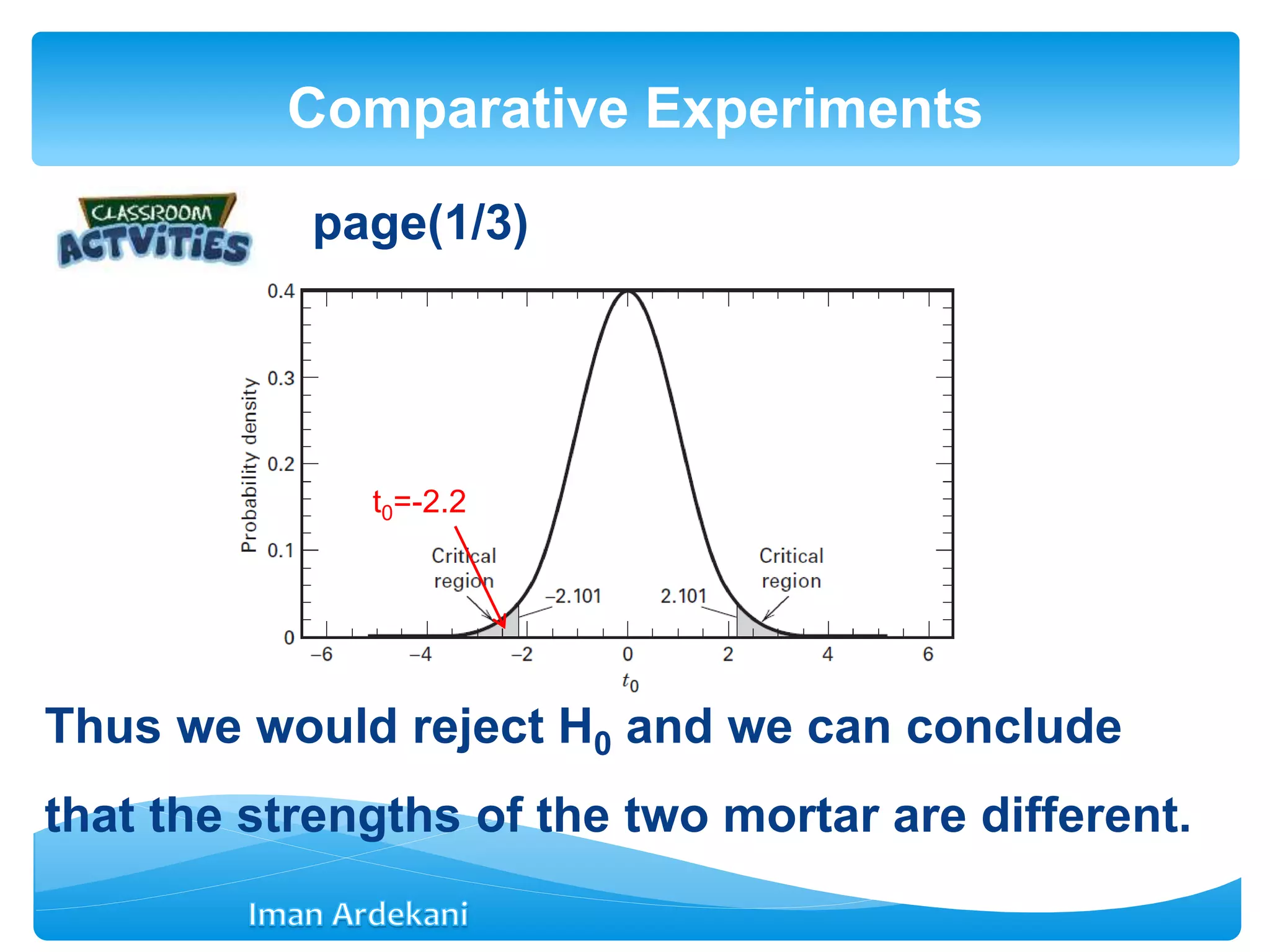
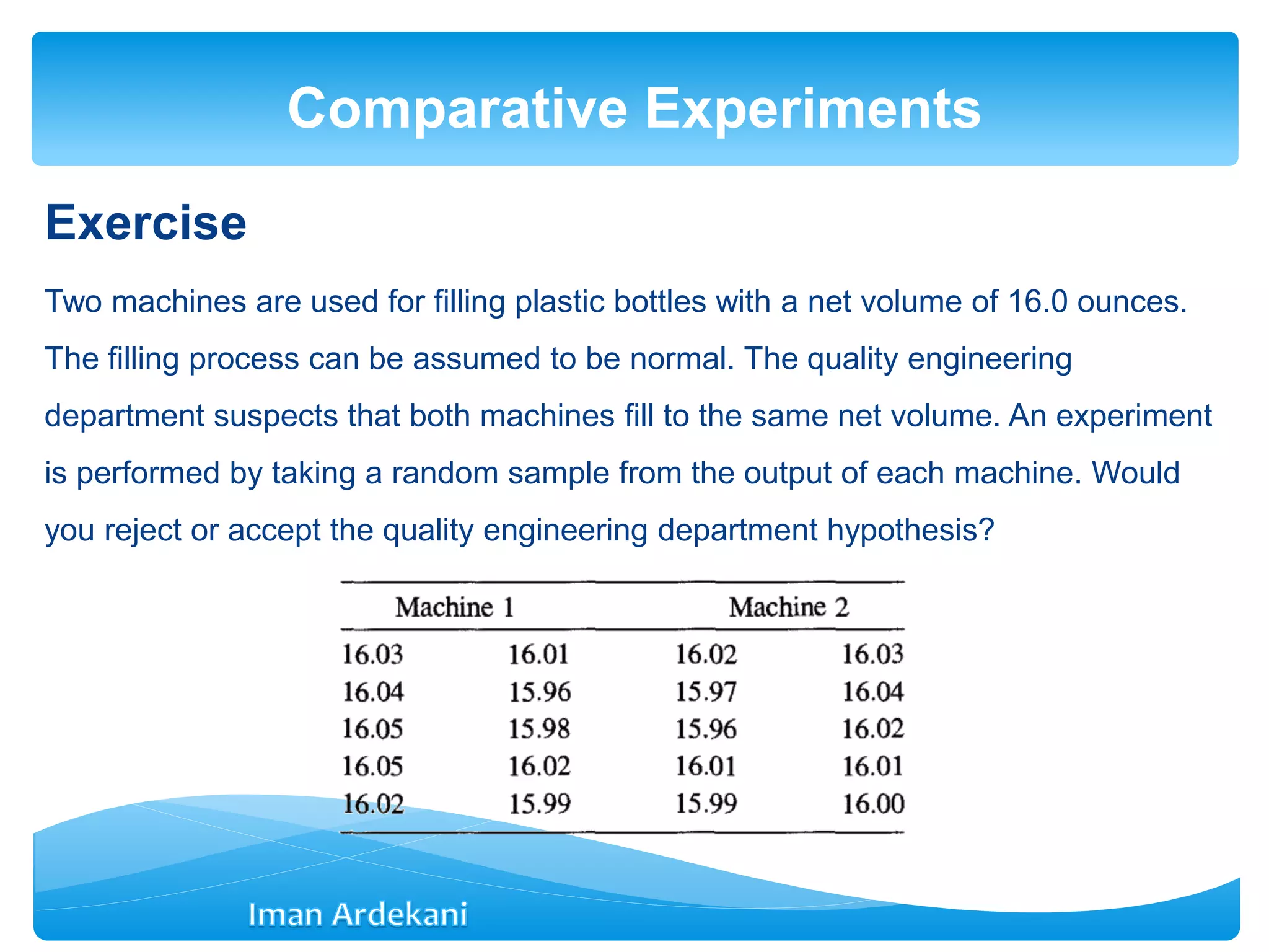
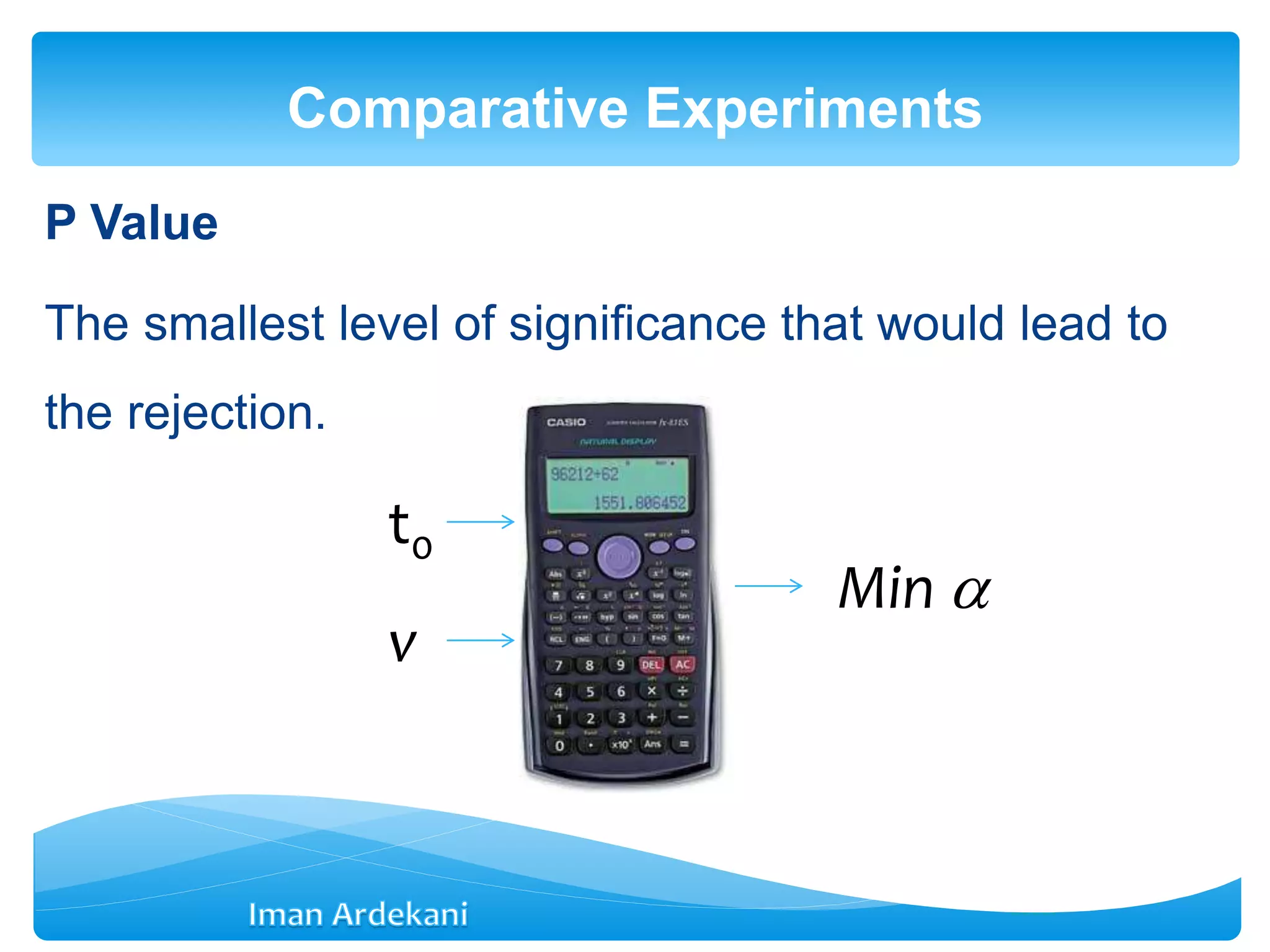
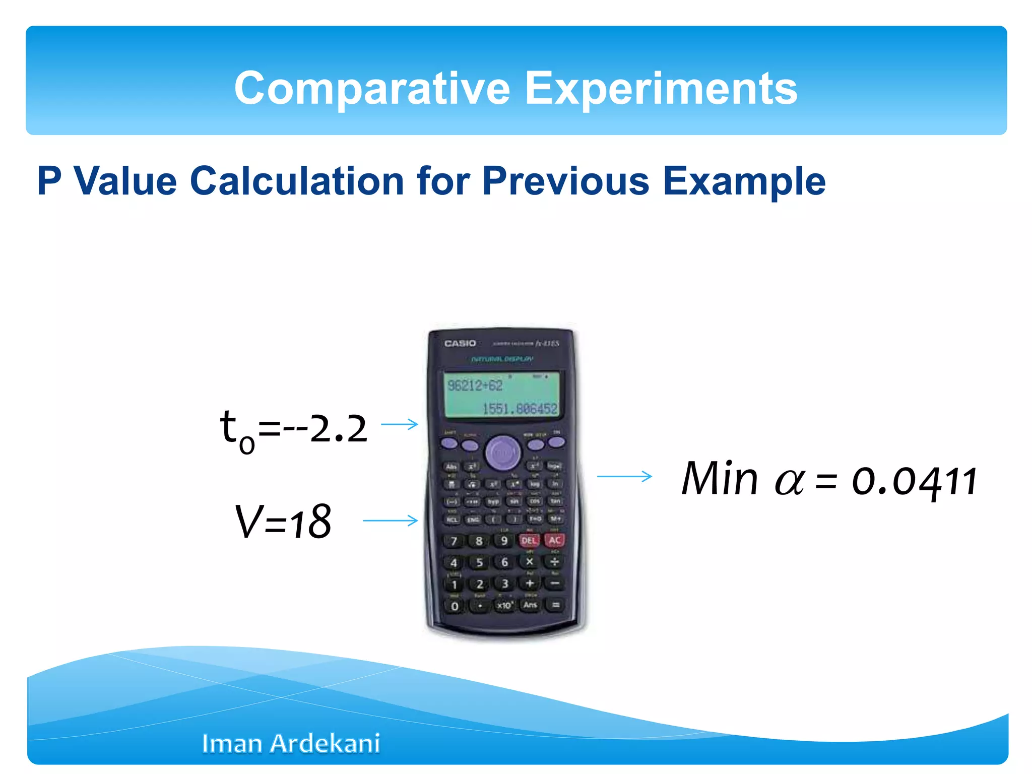
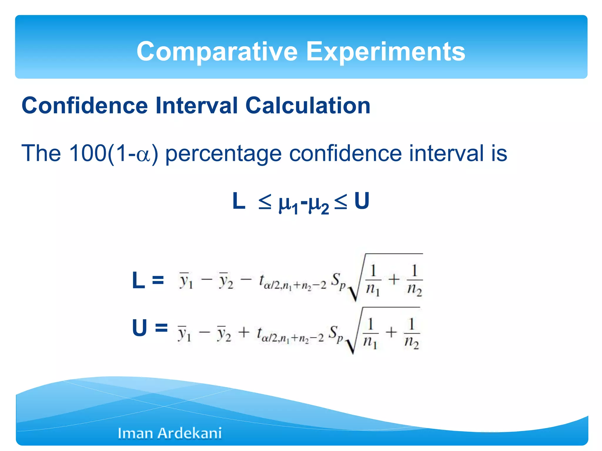
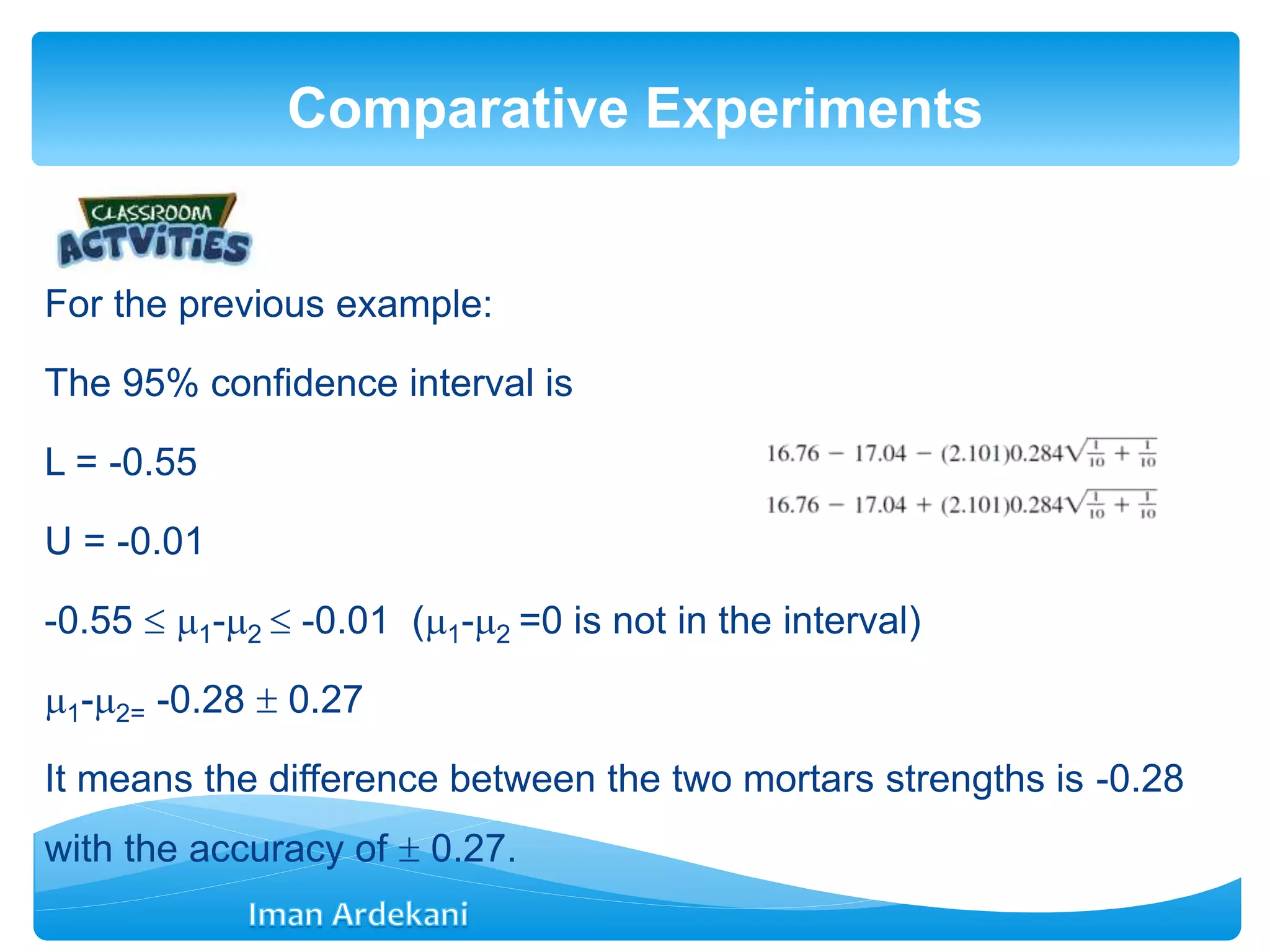
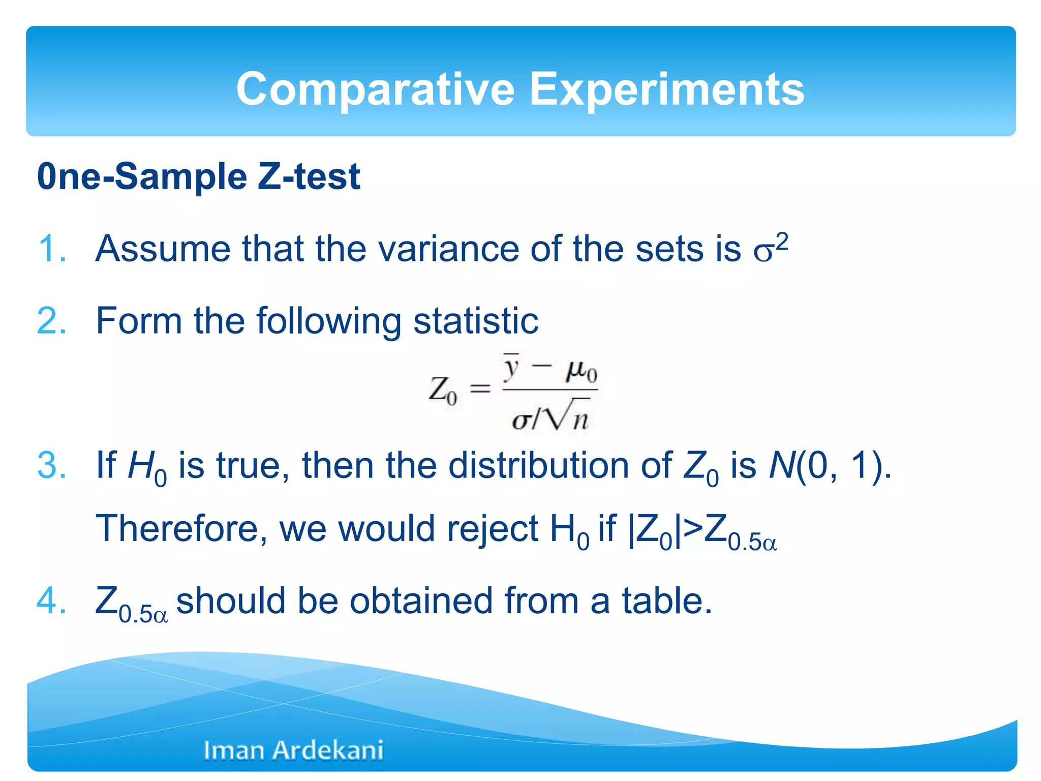
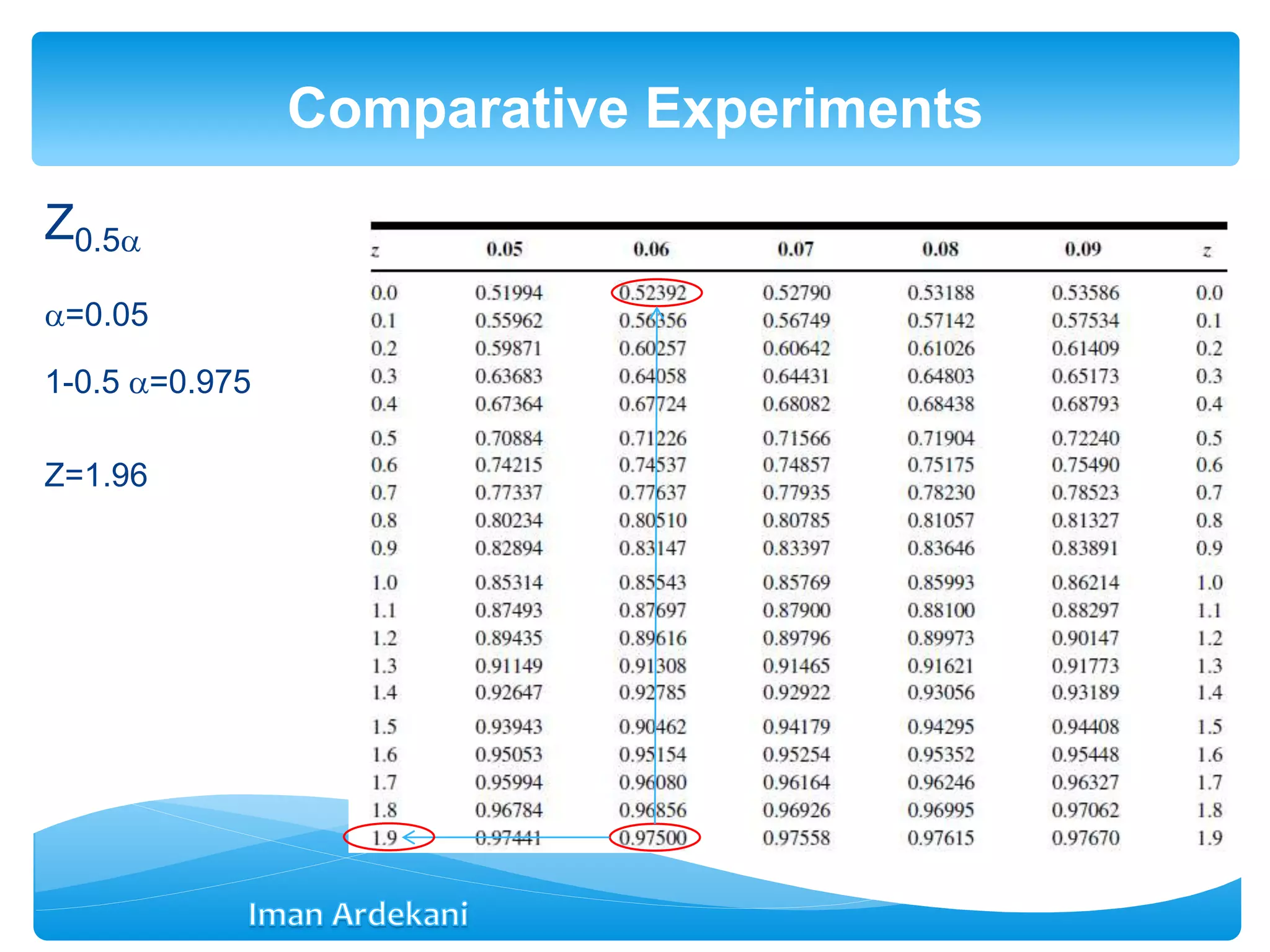
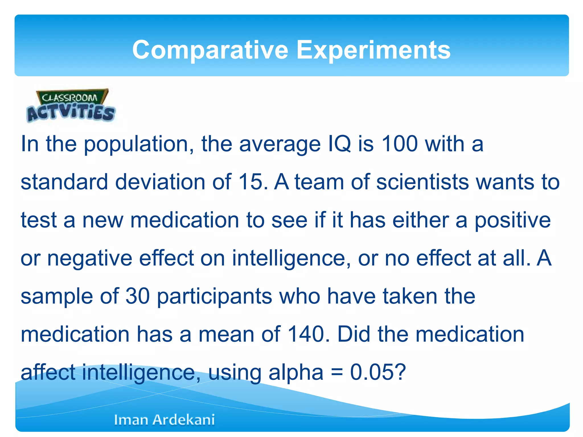
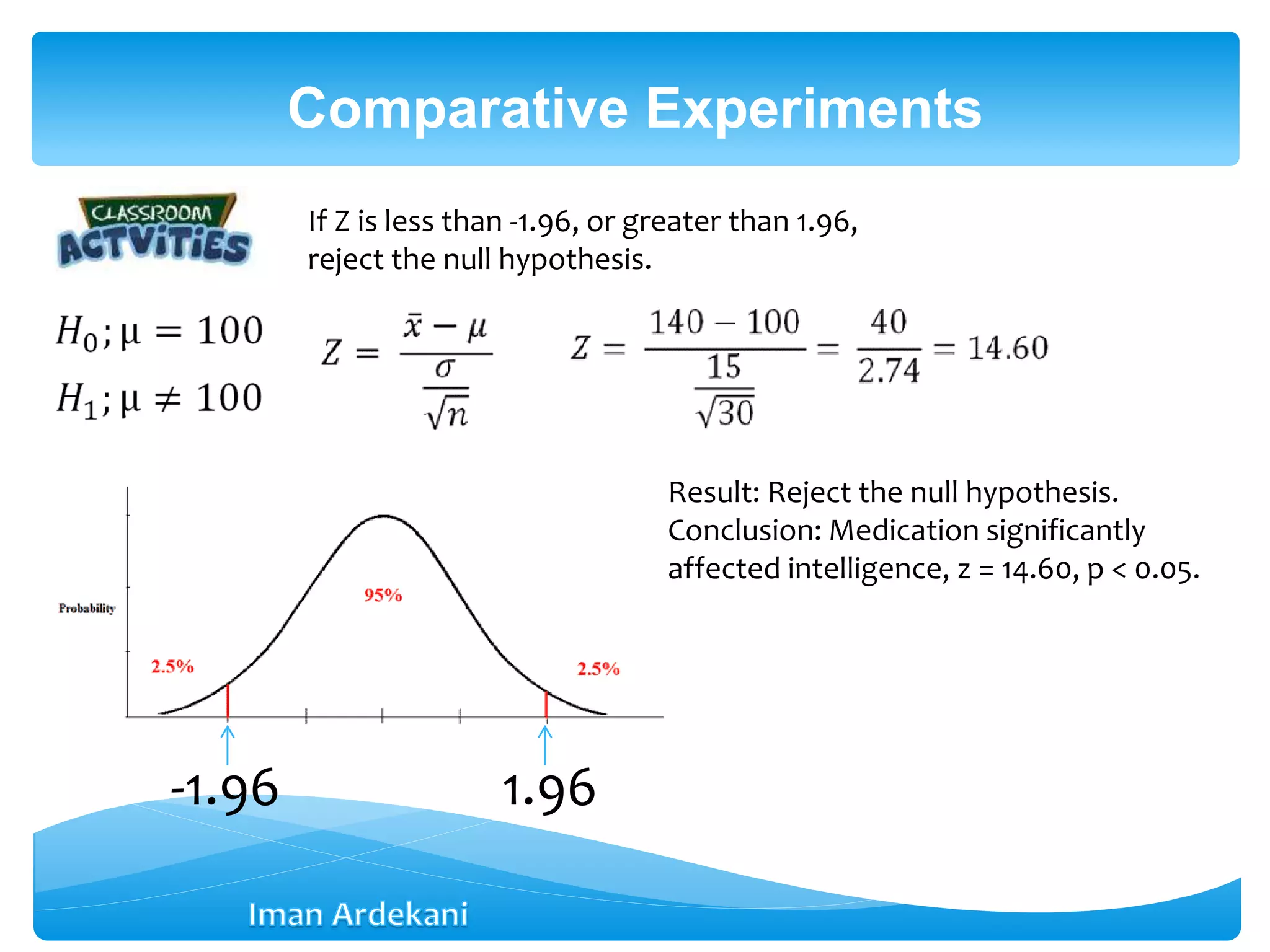
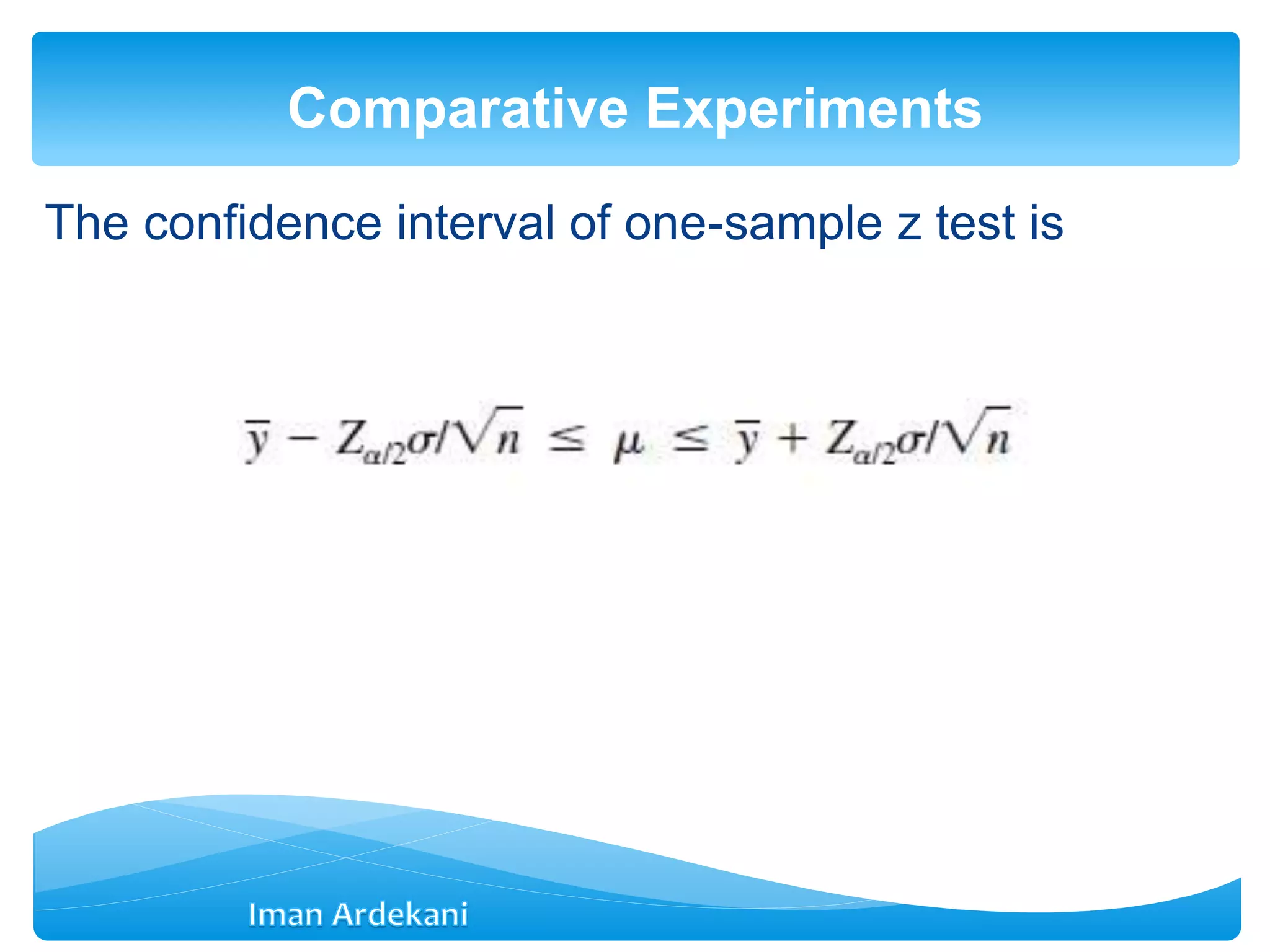
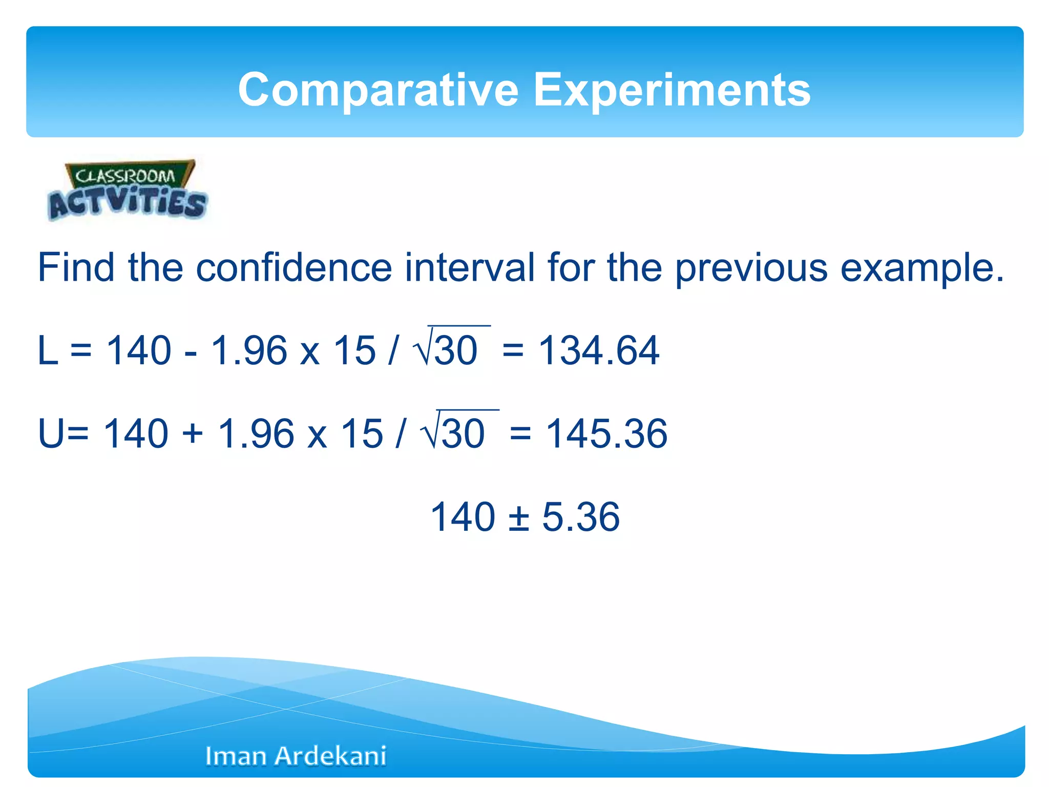
Addresses comparative experiments, formulates hypotheses, discusses two-sample t-tests, P-values, confidence intervals, and violations of assumptions.
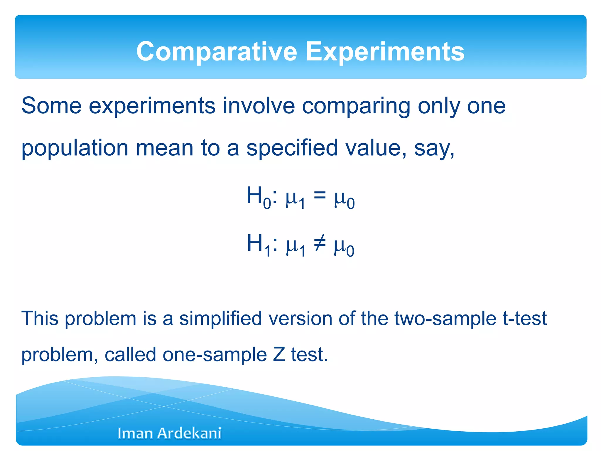
Presents results from a one-sample Z test, outlines confidence intervals, and addresses assumptions impacting the validity of tests.