The document outlines advancements in medical imaging, focusing on compressed sensing (CS) techniques to improve MRI data acquisition and reconstruction efficiency. It discusses various MRI protocols, challenges of long acquisition times, and emphasizes the potential for reducing acquisition time by 75% without compromising data fidelity. Additionally, it highlights the implementation of CS in metabolic imaging and dynamic contrast-enhanced MRI, showcasing improved spatial and temporal resolutions in diagnostic evaluations.

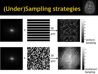
1. Sairam Geethanath, Ph.D.
Medical Imaging Research Centre
Dayananda Sagar Institutions,
Bangalore

2. Speed
Data provided by Baek
Contrast
SNR
MRI

3. ¡ Number of non-zero coefficients in a data
vector
¡ Importance due to conservation of energy
¡ Sinusoidal signal for 3 hours in time
domain or frequency domain?
¡ Move towards time-frequency transforms

4. ¡ CS: what is it all about?
¡ Matlab demo
¡ Steps ahead on CS
¡ Resources on CS

5. ¡ Childlike question on compression
¡ Acceleration technique involving both
acquisition and reconstruction paradigms
¡ Technically challenging, pragmatically
feasible and clinically valuable

6. • Good data quality but takes a long time!
• Hence, may not be suitable for certain imaging protocols.
• Limits spatial and temporal resolutions
• Higher spatial resolution aids in morphological analysis of
tumors – breast DCE-MRI
• Temporal resolution is important for accurate
pharmacokinetic analysis.
• Several approaches like keyhole, parallel imaging and other
fast sequences have been used.2D FFT
2D
IFFT
50
100
150
200
X
1 0 Data provided by Baek

7. X
2D
IFFT
10
20
30
40
50
60
70
10
20
30
40
50
60
70
Uniform
Sampling
X
2D
IFFT
20
40
60
80
100
120
20
40
60
80
100
120
Incoherent
Sampling

8. Complete data reconstruction
Wavelet
Transform
Data provided by Baek
[1] David L. Donoho, IEEE Transactions on Information theory, Vol.52, no. 4, April 2006
[2] Candes, E.J. et al., IEEE Transactions on Information theory, Vol.52, no.2, Feb. 2006
• Most objects in nature are approximately sparse in a transformed domain.
• Utilize above concept to obtain very few measurements and yet reconstruct
with high fidelity [1,2]
Only 33% of complete
data
X

9. 50 100 150 200 250
0
2
4
6
8
10
Sparse vector for recon
0 50 100 150 200 250 300
0
5
10
15
20
25
Kspace of 1D signal
50 100 150 200 250
0
0.2
0.4
0.6
0.8
1
1.2
Equi-spaced Recon
50 100 150 200 250
0
0.5
1
Rand Recon
50 100 150 200 250
0
0.5
1
Thresholded peaks
50 100 150 200 250
0
0.5
1
Interference of Thresholded peaks
0 50 100 150 200 250 300
0
0.05
0.1
0.15
0.2
0.25
Recovery of comp under noise floor
50 100 150 200 250
0
0.5
1
CS recon of the three components - scaled

10. ¡ Generate a 2D phantom
¡ Cartesian undersampling of data
¡ Obtain undersampled data and zfwdc recon
¡ Choice of ROI if required for diagnostic evaluation purposes
¡ Recon params, post L-curve optimization
¡ Nonlinear conjugate gradient iterative reconstruction
¡ Comparative quality

11. Point spread
function analyses
1. Incoherence
2. Design of this
sampling mask

12. K-space
trajectories with 2
constraints:
1. Slew rate
2. Smoothness of
k-space
coverage

13. ¡ Every MRI method:
§ Angiography
§ DWI/DTI/SWI/DCE-MRI/ASL
§ fMRI/MRSI/CMR
§ ….
¡ Because MRI is inherently a slow acquisition
process, mostly dictated by the physics of
acquisition
¡ Magnetic Resonance Fingerprinting

14. 1. Rapid 1H MR metabolic imaging
2. Accelerated DCE-MRI
3. Swifter Sweep Imaging with Fourier Transform (SWIFT)
MRI

15. ¡ It has been well established that magnetic resonance imaging (MRI)
provides critical information about cancer [3].
¡ Magnetic resonance spectroscopic imaging (MRSI) furthers this
capability by providing information about the presence of certain
‘metabolites’ which are known to be important prognostic markers
of cancer [4] (stroke, AD, energy metabolism, TCA cycle).
¡ MRSI provides information about the spatial distribution of these
metabolites, hence enabling metabolic imaging.
[3] Huk WJ et al., Neurosurgical Review 7(4) 1984;
[4] Preul MC et al., Nat. Med. 2(3) 1996;

16. ¡ Increased choline level
¡ Reduced
N-Acetylaspartate (NAA)
level
¡ Reduced creatine level
[5] H Kugel et al., Radiology 183 June 1992
[5]
CANCER
NORMAL

17. ¡ Long acquisition times for MRSI
§ A typical MRSI protocol (32 X 32 X 512) takes ~ 20 minutes
§ Difficult to maintain anatomical posture for long time
§ Increases patient discomfort, likelihood of early termination of study
§ Discourages routine clinical use of this powerful MRI technique
¡ To increase throughput (decreased scanner time, technician time)
¡ Reduction of acquisition time is usually accomplished by under
sampling measured data (k-space).
¡ Limitations of Shannon-Nyquist criterion.
¡ Compressed sensing provides a framework to achieve sub-Nyquist
sampling rates with good data fidelity.

18. Brain - normal
(N=6)
Brain - cancer
(N=2)
Prostate -cancer
(N=2)
MRSI data Scanner TR(ms) TE(ms) # Averages Grid Size FOV (mm3)
Brain - normal
(N=6)
Siemens 3.0T
Trio Tim
1700 270 4 16 x 16 x 1024 100 x 100 x 15
Brain cancer
(N=2)
Philips 3.0T
Achieva
1000
112
112
2
2
18 x 21 x 1024
19 x 22 x 1024
180 x 210 x15
190 x 220 x 15
Prostate cancer
(N=2)
Philips 3.0T
Achieva
1200
1000
140
140
1
1
14 x 10 x 1024
16 x 12 x 1024
25 x 50 x 33
20 x 51 x 26

19. ¡ Minimal data processing done using jMRUI [7]
¡ FID Apodization – Gaussian (~3Hz)
¡ Removal of water peak using HLSVD
¡ Phase correction
§ To allow correct integration of the real part of the spectra
¡ QUEST based quantitation. [8]
§ To generate specific metabolite maps.
[7] A. Naressi, et al., Computers in Biology and Medicine, vol. 31, 2001.
[8] H. Ratiney, et al., Magnetic Resonance Materials in Physics Biology and Medicine, vol. 16, 2004.

20. 1X
NAACr
Cho
5X

21. Brain cancer
1X
2X
5X
10X
Prostate cancer
Normal CancerNormal Cancer
NAACr
ChoNAA
Cr
Cho
Cr2 Cr2 Cr
Cho
Cit Cit
Cho
+ Cr

22. Brain - cancer
Prostate - cancer
Brain - Normal Metabolite maps

23. § Mean ± SD of pooled
data for each data
type
§ 2 tailed paired
t-test
§ Ratio: CNI for brain
data and (Cho + cr)/
Cit for prostate data
§ Excluded voxels with
denominator value
of 0 in 1X case
§ For CS cases, if the
denominator had a
value of 0, the ratio
was set to 0
§ P value less than
0.05 was chosen as a
significant
difference
(* p <0.05)
NAA
(a.u.)
Cr
(a.u.)
Cho
(a.u.)
Cit
(a.u.)
Ratio
Brain
(Normal)
1X 200 ± 96.8 51.83 ± 27.6 13.8 ± 8.87 0.075 ± 0.047
2X 200 ± 98.9 51.99 ± 34.5 13.8 ± 10.2 0.073 ± 0.064
5X 202 ± 110 51.71 ± 30.7 13. 9 ± 10.6 0.082 ± 0.152
10X 241 ± 138* 65.22 ± 39.3* 17.9 ± 13.2* 0.086 ± 0.083*
Brain
(Cancer)
1X 10.7 ± 6.35 4.23 ± 2.43 3.21 ± 1.38 0.468 ± 0.519
2X 10.8 ± 6.45 4.27 ± 2.60 3.21 ± 1.37 0.625 ± 1.50
5X 10.6 ± 7.42 4.19 ± 2.35 3.21 ± 1.36 0.712 ± 1.82
10X 11.1 ± 8.78 3.72 ± 1.72* 3.27 ± 1.47 0.837 ± 1.89*
Prostate
(Cancer)
1X 499 ± 821 2010 ± 1730 188 ± 166 19.25 ± 25.23
2X 427 ± 830 1850 ± 1460 194 ± 131 14.10 ± 10.21
5X 382 ± 541 1830 ± 1450 193 ± 131 16.12 ± 16.44
10X 378 ± 540 1470 ± 958* 135 ± 111* 16.38 ± 23.59

24. N = total number of elements of the MRSI data;
Θ, Θ’ = the data reconstructed from full k-space and undersampled k-space respectively.
∑=
Θ−Θ=
N
i
ii
N
RMSE
1
2
)'(
1
'

25. ¡ Application of compressed sensing on 1H MRSI has been performed for the
first time
¡ It has been demonstrated that compressed sensing based reconstruction can
be successfully applied on 1H MRSI in vivo human brain (normal and cancer),
prostate cancer data and in vitro, computer generated phantom data sets
¡ Our results indicate a potential to reduce MRSI acquisition times by 75%
thus significantly reducing the time spent by the patient in the MR
scanner for spectroscopic studies
¡ Current and future work involves the implementation of compressed sensing
based pulse sequences on preclinical and clinical scanners
¡ Other groups in the world are working on this demonstration now!

26. ¡ Rapid 1H MR metabolic imaging
¡ Accelerated DCE-MRI
¡ Swifter Sweep Imaging with Fourier
Transform (SWIFT) MRI

27. C(t) =
f(ΔR1(t))
T1 – weighted
images for
baseline
T1 shortening
contrast agent
[10] Yankeelov TE, et. al MRI;23(4). 2005
*Model implemented by Dr. Vikram Kodibagkar in MATLAB
[10]
Tissue perfusion, microvascular
density and
extravascular -extracellular
volume -- tumor staging,
monitor treatment response

28. Spre(ω) = Lpre(ω) + Hpre(ω) (1a)
Spost(ω) = Lpost(ω) + Hpre(ω) (1b)
Є( Idiff) = || FIdiff – ydiff||2 + λLI || WIdiff ||1 +λTV(Idiff) (2)
Keyhole for DCE
CS for DCE
Ipost-contrast Ipre-contrast Idiff
Data was
normalized to a
range of 0 to 1
before
retrospective
reconstruction
Spost(ω) Spre(ω) ydiff
[11] Vanvaals JJ et. al. JMRI; 3(4) 1993
[12] Jim J et. al. IEEE TMI 2008
[13] Lustig M et. al. MRM;58(6) 2007
[11]
[12,13]

29. ¡ 5 DCE-MRI breast cancer data sets consisting of 64 frames (4 pre-
contrast images and 60 post-contrast images) were used for
retrospective reconstructions.
¡ The contrast agent used was Omniscan (intravenously administered
through the tail vein at a dose of 0.1 mmol/kg).
¡ Reconstructions based on 2 approaches: keyhole and compressed
sensing, were performed as function of masks and acceleration
factors were performed.
¡ These reconstructions were quantified by the root mean square error
metric defined below
∑=
Θ−Θ=
N
i
ii
N
RMSE
1
2
)'(
1
'

30. 5X4X3X2X
CS_Gauss
Keyhole
CS_Glines
CS_Thresh
Keylines
Keythresh
Original
5X4X3X2X
Masks Recon

31. Starts at frame 1 Starts at frame 6 (post-contrast)
Keyhole CS
Keyhole
Keylines
Keythresh
CS_Gauss
CS_Glines
CS_Thresh

32. 5X4X3X2X
CS_Gauss
Keyhole
CS_Glines
CS_Thresh
Keylines
Keythresh
Original
5X4X3X2X
Ktrans Ve

33. T2w Overlay
T1w
pre-
contrast
T1w
post-
contrast
0 10 20 30 40 50 60
0.150
0.175
0.200
0.225
0.250
ROIIntensity
Frame #
Original Keyhole Keylines Keythresh
Gauss Glines Gthresh
Muscle
0 10 20 30 40 50 60
0.175
0.200
0.225
0.250
ROIIntensity
Frame #
Original Keyhole Keylines Keythresh
Gauss Glines Gthresh
Poorly perfused region
0 10 20 30 40 50 60
0.15
0.20
0.25
0.30
0.35
0.40
ROIIntensity
Frame #
Original Keyhole Keylines Keythresh
Gauss Glines Gthresh
Well perfused region

34. Muscle
Well perfused Poorly perfused

35. ¡ It has been shown here and previously that DCE MRI can be
reliably accelerated through methods like compressed sensing and
keyhole reconstructions to obtain increased spatial and/or
temporal resolution.
¡ CS based masks – Gauss and Gthresh provide better performance
when compared to Glines mask, which out do the keyhole masks
as observed by the RMSE graphs.
¡ Keyhole based masks – keyhole mask performs relatively poorer
when compared to keythresh and keylines masks
¡ Acceleration factors – the values of RMSE increases with
acceleration as expected (not shown); the CS masks show a RMSE
of less than 0.075 even at an acceleration factor of 5 while
keyhole masks result in a RMSE of less than 0.1

36. ¡ Rapid 1H MR metabolic imaging
¡ Accelerated DCE-MRI
¡ Swifter Sweep Imaging with Fourier
Transform (SWIFT) MRI

37. [14] D.Idiyatullin et al., JMR, 181, 2006. [14]
§ Sweep imaging with Fourier transformation [14]
§ Time domain signals are acquired during a swept radiofrequency
excitation in a time shared way
§ This results in a significantly negligible echo time.
§ Insensitive to motion, restricted dynamic range, low gradient noise
GRE SWIFT Photograph
Bovine tibia

38. ¡ Full k-space recon was performed using gridding. The volume was restricted
to a range of [0,1] by normalizing it to the highest absolute value.
¡ Prospective implementation is straight forward due to the nature of k-space
trajectory. Acceleration of 5.33 X was achieved – directly proportional to time
saved
¡ MR data is sparse in the total variation domain. Since the data in this case is
3D, a 3D total variation norm is most apt.
¡ Reconstruction involves minimization of the convex functional given below.
This is accomplished by a custom implementation of non-linear conjugate
gradient algorithm.
Є(m) = || Fum – y||2 +λTV TV(m)
where m is the desired MRI volume,
Fu is the Fourier transform operator,
TV is the 3D total variation operator,
||.||2 is the L2 norm operator,
λTV is the regularization parameter for the TV term respectively, and
Є is the value of the cost function.

39. ¡ The initial estimate of the volume is given by the zero-filled case with
density compensation (zfwdc). This produces artifacts which are
incoherent as can be seen in the zfwdc images.
¡ A total of 8 iterations were used and the recon was performed in 4 mins.
¡ NRMSE given by RMSE/ range of input; i.e. 1; hence NRMSE = RMSE
calculated as given below
N = total number of elements of the MRI volume; Θ, Θ’= the data reconstructed from full k-
space and undersampled k-space respectively.
∑=
Θ−Θ=
N
i
ii
N
RMSE
1
2
)'(
1
'

40. Original
5.33 X
Zero filled
with density
compensation

41. 50 100 150
0.0
0.2
0.4
0.6
Pixel number
Intensity(au)
Original
5X
Zero filled
with density
compensation
(Zfwdc) 50 100 150
0.0
0.2
0.4
0.6
Pixel Number
Intensity(au)
50 100 150
0.0
0.2
0.4
0.6
Pixel Number
Intensity(au)

42. Original 5X
Scan time ~ 8 min Estimated scan time ~1.6 min

43. Original
5 X
Zfwdc

44. ¡ “Review on CS MRI” Critical reviews in
biomedical engineering 2013
¡ http://nuit-blanche.blogspot.in/
¡ Miki Lustig, UC Berkley
¡ John M Pauly, Stanford
¡ www.ismrm.org

45. ¡ 25+ member team (14 + 11’)
¡ Impact factor > 15 for 2012 – 13
¡ Considered world experts in CS
¡ Work on CS has been showcased in the American Society
of Neuroradiologists 2013 annual conference
¡ Several groups worldwide are working on our idea
including Oxford and Yale
¡ http://www.dayanandasagar.edu/mirc-home.html

47. Human Scan
o Scanning Started from: 5-07-2013
o Number of volunteers scanned till 18-08-2013: 20

48. PEOPLE
§ Dr. Vikram D. Kodibagkar
§ CSI project
§ Hyeonman Baek, Ph.D.
§ Matthew Lewis, Ph.D.
§ Sandeep K. Ganji, B. Tech.
§ Yao Ding, M.S.
§ Robert D. Sims, M.D.
§ Changho Choi, Ph.D.
§ Elizabeth Maher, M.D., Ph.D.
§ DCE project
§ Praveen K. Gulaka, M.S.
§ SWIFT project
§ Matthew Lewis, Ph.D.
§ Steen Moeller, Ph.D.
§ Curtis A. Corum, Ph.D.
FUNDING
§ Pilot grant (PI: Kodibagkar) from
UL1RR024982, (PI: Milton Packer)
§ ARP#010019-0056-2007 (PI: Kodibagkar)
§ R21CA132096-01A1 (PI: Kodibagkar)
§ W81XWH-05-1-0223 (PI: Kodibagkar)
§ R21 CA139688 (PI: Corum)
§ S10 RR023730 (PI: Garwood)
§ P41 RR008079 (PI: Garwood)

49. ¡ Mr. Rajesh Harsh, Mr. Ravindran Nair,
Mr. T.S. Datta, Mr. R.S.Verma
¡ MIRC students
¡ Knowledge partners for MRI India Consortium:
AIIMS, Harvard, NYU, Minnesota, Auburn
¡ ASU, KCL/ICL, Wipro-GE Healthcare
¡ Scientists/Participants
¡ Management of DSCE