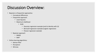
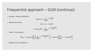
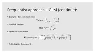
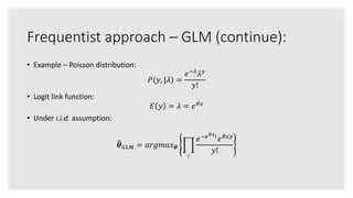
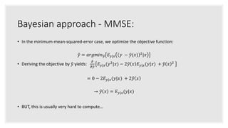
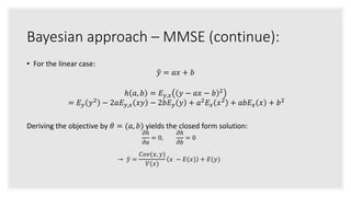
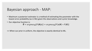
SlideShare a Scribd company logo
Statistical Signal
Processing
Nadav Carmel
Discussion Overview:
• Bayesian vs frequentist approaches:
• Conceptual differences
• Frequentist approach:
• Least-Squares
• Maximum-Likelihood
• GLM:
• Gaussian regression example (and its identity with LS)
• Bernoulli regression example (Logistic regression)
• Poisson regression example
• Bayesian approach:
• MMSE
• MAP
• Online-learning algorithms:
• Kalman filter
• Perceptron
• Winnow
Bayesian vs frequentist approaches
• Frequentist:
• Understand probability as a frequency of a ‘repeatable’ events.
• Bayesian:
• Understand probability as a measure of a person’s degree of belief in an
event, given the information available.
Frequentist Approach – LS:
• We model the observations by:
𝑦 = 𝑓 𝒙, 𝜽 + 𝜀
• Then try to optimize the objective function
(ordinary least squares solution):
𝜽 𝐿𝑆 = 𝑎𝑟𝑔𝑚𝑖𝑛 𝜽
𝑖
𝑦𝑖 − 𝑓 𝒙𝒊, 𝜽
2
Ordinary (grey) and orthogonal
(red) LS
Frequentist Approach – LS (continue):
• For a linear model:
𝑦 = 𝒙 𝑇
𝜽 + 𝜀
• The optimization function becomes:
𝜽 𝐿𝑆 = 𝑎𝑟𝑔𝑚𝑖𝑛 𝜽
𝑖
𝑦𝑖 − 𝒙𝑖
𝑇
𝜽
2
Frequentist Approach – LS (continue):
• Solutions:
• For the linear case, analytical solution exists:
𝜽 𝐿𝑆 = 𝑋 𝑇
𝑋 −1
𝑋 𝑇
𝒚
• For non-linear cases, optimization is required. Is the problem convex??
𝛻𝜃
2
𝑒 =
𝑖
𝑒𝑖 𝛻𝜃
2
𝑒𝑖 +
𝑖
𝛻𝜃 𝑒𝑖 𝛻𝜃 𝑒𝑖
𝑇
=
𝑖
𝑒𝑖 𝛻𝜃
2
𝑒𝑖 + 𝐽 𝑇 𝐽
positiveDepends on f
Frequentist Approach – LS (continue):
• We can show for the linear case solution:
𝑋 𝑇 𝜺 = 𝑋 𝑇 𝒚 − 𝑋𝜃 = 𝑋 𝑇 𝒚 − 𝑋 𝑋 𝑇 𝑋 −1 𝑋 𝑇 𝒚 = 𝑋 𝑇 − 𝑋 𝑇 𝑋 𝑋 𝑇 𝑋 −1 𝑋 𝑇 𝒚 = 𝑋 𝑇 − 𝑋 𝑇 𝒚 = 𝟎
• => LS error is orthogonal to the feature space.
Frequentist Approach – LS (continue):
• Popular LS regularizations:
𝜽 𝐿𝑆 = 𝑎𝑟𝑔𝑚𝑖𝑛 𝜽
𝑖
𝑦𝑖 − 𝑓 𝒙𝒊, 𝜽
2
+ 𝜆 𝜃 𝑝
• P = 0: Compressed Sensing (NP hard combinatorial solution)
• P = 1: LASSO (convex, non differentiable)
• P=2: ridge regression (convex and differentiable)
Frequentist approach – ML:
• Maximum Likelihood – a method of estimating parameters from observations with lowest error
probability.
• We assume a distribution with the parameters vector 𝜽.
• We define an objective function to optimize - the joint distribution given the observations:
𝜽 𝑀𝐿 = 𝑎𝑟𝑔𝑚𝑎𝑥 𝜽 𝑃 𝑦1, 𝑦2, … , 𝑦𝑛|𝜽
Frequentist approach – ML (continue):
• Under the i.i.d. assumption:
𝜽 𝑀𝐿 = 𝑎𝑟𝑔𝑚𝑎𝑥 𝜽
𝑖
𝑃 𝑦𝑖|𝜽 = 𝑎𝑟𝑔𝑚𝑎𝑥 𝜽
𝑖
𝑙𝑜𝑔 𝑃 𝑦𝑖|𝜽
• Popular regularization form:
Akaike information criterion: 𝜽 𝑀𝐿 = 𝑎𝑟𝑔𝑚𝑎𝑥 𝜽 𝑖 𝑙𝑜𝑔 𝑃 𝑦𝑖|𝜽 − 𝑘 (k – the number of free parameters)
Frequentist approach - GLM:
• From Wiki:
“a flexible generalization of ordinary linear regression that allows for response
variables that have a distribution other than a normal distribution”.
• 3 components for GLM:
1. Response variable from a given distribution (as in ML).
2. Explanatory variables (features).
3. A link function to the expectancy response variable: 𝐸(𝑦) = 𝑓 𝑥, 𝜃 .
Frequentist approach – GLM (continue):
• We model the observations by:
𝑦 = 𝑓 𝒙, 𝜽 + 𝜀
• Then try to optimize the objective function (ordinary least squares solution):
𝜽 𝐺𝐿𝑀 = 𝑎𝑟𝑔𝑚𝑎𝑥 𝜽 𝑃 𝑦1, 𝑦2, … , 𝑦𝑛|𝒙 𝟏, 𝒙 𝟐, … , 𝒙 𝒏, 𝜽
• And under the i.i.d assumption:
𝜽 𝐺𝐿𝑀 = 𝑎𝑟𝑔𝑚𝑎𝑥 𝜽
𝑖
𝑃 𝑦𝑖|𝒙𝒊, 𝜽 = 𝑎𝑟𝑔𝑚𝑎𝑥 𝜽
𝑖
𝑙𝑜𝑔 𝑃 𝑦𝑖|𝒙𝒊, 𝜽
Frequentist approach – GLM (continue):
• Example – Gaussian distribution:
𝑃 𝑦|𝜇, 𝜎 =
1
2𝜋𝜎
𝑒
−
𝑦 −𝜇 2
2𝜎2
• Identity link function:
𝐸 𝑦 = 𝜇 = 𝑓 𝒙, 𝜽
→ 𝑃 𝑦𝑖|𝒙𝒊, 𝜽 =
1
2𝜋𝜎
𝑒
−
𝑦 𝑖 −𝑓 𝒙 𝒊,𝜽
2
2𝜎2
• Under i.i.d. assumption:
𝜽 𝐺𝐿𝑀 = 𝑎𝑟𝑔𝑚𝑎𝑥 𝜽
𝑖
1
2𝜋𝜎
𝑒
−
𝑦 𝑖 −𝑓 𝒙 𝒊,𝜽
2
2𝜎2
= 𝑎𝑟𝑔𝑚𝑖𝑛 𝜽
𝑖
𝑦𝑖 − 𝑓 𝒙𝒊, 𝜽
2
• Identical to the LS problem 
Frequentist approach – GLM (continue):
• Example – Bernoulli distribution:
𝑃(𝑦|𝑝) =
𝑝, 𝑦 = 1
1 − 𝑝, 𝑦 = 0
• Logit link function:
𝐸 𝑦 = 𝑝 =
𝑒 𝜃𝑥
1 + 𝑒 𝜃𝑥
• Under i.i.d. assumption:
𝜽 𝐺𝐿𝑀 = 𝑎𝑟𝑔𝑚𝑎𝑥 𝜽
𝑖
𝑒 𝜃𝑥
1 + 𝑒 𝜃𝑥
𝑦 𝑖
1 −
𝑒 𝜃𝑥
1 + 𝑒 𝜃𝑥
1−𝑦 𝑖
• A.K.A. Logistic Regression
Frequentist approach – GLM (continue):
• Example – Poisson distribution:
𝑃(𝑦, |𝜆) =
𝑒−𝜆
𝜆 𝑦
𝑦!
• Logit link function:
𝐸 𝑦 = 𝜆 = 𝑒 𝜃𝑥
• Under i.i.d. assumption:
𝜽 𝐺𝐿𝑀 = 𝑎𝑟𝑔𝑚𝑎𝑥 𝜽
𝑖
𝑒−𝑒 𝜃𝑥 𝑖
𝑒 𝜃𝑥𝑦
𝑦!
Frequentist approach – GLM (continue):
• Possible link functions and distribution families in Spark 2.1.0:
https://spark.apache.org/docs/2.1.0/ml-classification-regression.html#available-families
Bayesian approach - MMSE:
• In the minimum-mean-squared-error case, we optimize the objective function:
𝑦 = 𝑎𝑟𝑔𝑚𝑖𝑛 𝑦 𝐸 𝑦|𝑥 𝑦 − 𝑦(𝑥) 2|𝑥
• Deriving the objective by 𝑦 yields:
𝜕
𝜕 𝑦
𝐸 𝑦|𝑥(𝑦2
|𝑥) − 2 𝑦 𝑥 𝐸 𝑦|𝑥(𝑦|𝑥) + 𝑦 𝑥 2
= 0 − 2𝐸 𝑦|𝑥(𝑦|𝑥) + 2 𝑦 𝑥
→ 𝑦 𝑥 = 𝐸 𝑦|𝑥(𝑦|𝑥)
• BUT, this is usually very hard to compute…
Bayesian approach – MMSE (continue):
• For the linear case:
𝑦 = 𝑎𝑥 + 𝑏
ℎ 𝑎, 𝑏 = 𝐸 𝑦,𝑥 𝑦 − 𝑎𝑥 − 𝑏 2
= 𝐸 𝑦 𝑦2
− 2𝑎𝐸 𝑦,𝑥 𝑥𝑦 − 2𝑏𝐸 𝑦 𝑦 + 𝑎2
𝐸 𝑥 𝑥2
+ 𝑎𝑏𝐸 𝑥 𝑥 + 𝑏2
Deriving the objective by 𝜃 = (𝑎, 𝑏) yields the closed form solution:
𝜕ℎ
𝜕𝑎
= 0,
𝜕ℎ
𝜕𝑏
= 0
→ 𝑦 =
𝐶𝑜𝑣(𝑥, 𝑦)
𝑉(𝑥)
𝑥 − 𝐸(𝑥) + 𝐸(𝑦)
Bayesian approach - MMSE:
• By placing the general solution, we can see that:
𝐸 𝑦|𝑥 𝑦 − 𝑦 𝜃 ∗ 𝑥
= 𝐸 𝑦|𝑥 𝑦 − 𝐸 𝑦 𝑦 𝑥 ∗ 𝑥
= 𝐸 𝑦|𝑥 𝑦 ∗ 𝑥 − 𝐸 𝑦 𝑦 𝑥 ∗ 𝑥
= 0 (Bayes Law)
=> Orthogonality is preserved between the error and the features (similar to LS)
Bayesian approach - MAP:
• Maximum a posteriori estimator is a method of estimating the parameter with the
lowest error probability (as in ML) given the observations and a prior knowledge.
• Our objective function is:
𝜽 = 𝑎𝑟𝑔𝑚𝑎𝑥 𝜽 𝑃(𝜽|𝒙) = 𝑎𝑟𝑔𝑚𝑎𝑥 𝜽 𝑃 𝒙 𝜽 ∗ 𝑃(𝜽)
=> When our prior in uniform, the objective is exactly identical to ML.

More Related Content

What's hot

Algebra Presentation on Topic Modulus Function and Polynomials
Algebra Presentation on Topic Modulus Function and PolynomialsAlgebra Presentation on Topic Modulus Function and Polynomials
Algebra Presentation on Topic Modulus Function and Polynomials
AsukaMiyanomae
 
Gauss Jordan
Gauss JordanGauss Jordan
Gauss Jordan
Ezzat Gul
 
Connected components and shortest path
Connected components and shortest pathConnected components and shortest path
Connected components and shortest path
Kaushik Koneru
 
INVERSION OF MATRIX BY GAUSS ELIMINATION METHOD
INVERSION OF MATRIX BY GAUSS ELIMINATION METHODINVERSION OF MATRIX BY GAUSS ELIMINATION METHOD
INVERSION OF MATRIX BY GAUSS ELIMINATION METHOD
reach2arkaELECTRICAL
 
Numerical Methods
Numerical MethodsNumerical Methods
Numerical Methods
tesfahun meshesha
 
Solving Poisson Equation using Conjugate Gradient Method and its implementation
Solving Poisson Equation using Conjugate Gradient Methodand its implementationSolving Poisson Equation using Conjugate Gradient Methodand its implementation
Solving Poisson Equation using Conjugate Gradient Method and its implementation
Jongsu "Liam" Kim
 
BSC_COMPUTER _SCIENCE_UNIT-4_DISCRETE MATHEMATICS
BSC_COMPUTER _SCIENCE_UNIT-4_DISCRETE MATHEMATICSBSC_COMPUTER _SCIENCE_UNIT-4_DISCRETE MATHEMATICS
BSC_COMPUTER _SCIENCE_UNIT-4_DISCRETE MATHEMATICS
Rai University
 
Lecture 5 (solving simultaneous equations)
Lecture 5 (solving simultaneous equations)Lecture 5 (solving simultaneous equations)
Lecture 5 (solving simultaneous equations)
HarithaRanasinghe
 
EASY WAY TO CALCULATE MODE (STATISTICS)
EASY WAY TO CALCULATE MODE (STATISTICS)EASY WAY TO CALCULATE MODE (STATISTICS)
EASY WAY TO CALCULATE MODE (STATISTICS)
sumanmathews
 
GAUSS ELIMINATION METHOD
 GAUSS ELIMINATION METHOD GAUSS ELIMINATION METHOD
GAUSS ELIMINATION METHOD
reach2arkaELECTRICAL
 
Gauss Elimination & Gauss Jordan Methods in Numerical & Statistical Methods
Gauss Elimination & Gauss Jordan Methods in Numerical & Statistical MethodsGauss Elimination & Gauss Jordan Methods in Numerical & Statistical Methods
Gauss Elimination & Gauss Jordan Methods in Numerical & Statistical Methods
Janki Shah
 
Gauss sediel
Gauss sedielGauss sediel
Gauss sediel
jorgeduardooo
 
Lecture 6.1 6.2 bt
Lecture 6.1 6.2 btLecture 6.1 6.2 bt
Lecture 6.1 6.2 bt
btmathematics
 
A uniform distribution has density function find n (1)
A uniform distribution has density function find n (1)A uniform distribution has density function find n (1)
A uniform distribution has density function find n (1)
Nadeem Uddin
 
تطبيقات المعادلات التفاضلية
تطبيقات المعادلات التفاضليةتطبيقات المعادلات التفاضلية
تطبيقات المعادلات التفاضلية
MohammedRazzaqSalman
 
Numerical Analysis and Its application to Boundary Value Problems
Numerical Analysis and Its application to Boundary Value ProblemsNumerical Analysis and Its application to Boundary Value Problems
Numerical Analysis and Its application to Boundary Value Problems
Gobinda Debnath
 
Gauss jordan
Gauss jordanGauss jordan
Gauss jordan
jorgeduardooo
 
Comparative analysis of x^3+y^3=z^3 and x^2+y^2=z^2 in the Interconnected Sets
Comparative analysis of x^3+y^3=z^3 and x^2+y^2=z^2 in the Interconnected Sets Comparative analysis of x^3+y^3=z^3 and x^2+y^2=z^2 in the Interconnected Sets
Comparative analysis of x^3+y^3=z^3 and x^2+y^2=z^2 in the Interconnected Sets
Vladimir Godovalov
 
Properties of coefficient of correlation
Properties of coefficient of correlationProperties of coefficient of correlation
Properties of coefficient of correlation
Nadeem Uddin
 

What's hot (19)

Algebra Presentation on Topic Modulus Function and Polynomials
Algebra Presentation on Topic Modulus Function and PolynomialsAlgebra Presentation on Topic Modulus Function and Polynomials
Algebra Presentation on Topic Modulus Function and Polynomials
 
Gauss Jordan
Gauss JordanGauss Jordan
Gauss Jordan
 
Connected components and shortest path
Connected components and shortest pathConnected components and shortest path
Connected components and shortest path
 
INVERSION OF MATRIX BY GAUSS ELIMINATION METHOD
INVERSION OF MATRIX BY GAUSS ELIMINATION METHODINVERSION OF MATRIX BY GAUSS ELIMINATION METHOD
INVERSION OF MATRIX BY GAUSS ELIMINATION METHOD
 
Numerical Methods
Numerical MethodsNumerical Methods
Numerical Methods
 
Solving Poisson Equation using Conjugate Gradient Method and its implementation
Solving Poisson Equation using Conjugate Gradient Methodand its implementationSolving Poisson Equation using Conjugate Gradient Methodand its implementation
Solving Poisson Equation using Conjugate Gradient Method and its implementation
 
BSC_COMPUTER _SCIENCE_UNIT-4_DISCRETE MATHEMATICS
BSC_COMPUTER _SCIENCE_UNIT-4_DISCRETE MATHEMATICSBSC_COMPUTER _SCIENCE_UNIT-4_DISCRETE MATHEMATICS
BSC_COMPUTER _SCIENCE_UNIT-4_DISCRETE MATHEMATICS
 
Lecture 5 (solving simultaneous equations)
Lecture 5 (solving simultaneous equations)Lecture 5 (solving simultaneous equations)
Lecture 5 (solving simultaneous equations)
 
EASY WAY TO CALCULATE MODE (STATISTICS)
EASY WAY TO CALCULATE MODE (STATISTICS)EASY WAY TO CALCULATE MODE (STATISTICS)
EASY WAY TO CALCULATE MODE (STATISTICS)
 
GAUSS ELIMINATION METHOD
 GAUSS ELIMINATION METHOD GAUSS ELIMINATION METHOD
GAUSS ELIMINATION METHOD
 
Gauss Elimination & Gauss Jordan Methods in Numerical & Statistical Methods
Gauss Elimination & Gauss Jordan Methods in Numerical & Statistical MethodsGauss Elimination & Gauss Jordan Methods in Numerical & Statistical Methods
Gauss Elimination & Gauss Jordan Methods in Numerical & Statistical Methods
 
Gauss sediel
Gauss sedielGauss sediel
Gauss sediel
 
Lecture 6.1 6.2 bt
Lecture 6.1 6.2 btLecture 6.1 6.2 bt
Lecture 6.1 6.2 bt
 
A uniform distribution has density function find n (1)
A uniform distribution has density function find n (1)A uniform distribution has density function find n (1)
A uniform distribution has density function find n (1)
 
تطبيقات المعادلات التفاضلية
تطبيقات المعادلات التفاضليةتطبيقات المعادلات التفاضلية
تطبيقات المعادلات التفاضلية
 
Numerical Analysis and Its application to Boundary Value Problems
Numerical Analysis and Its application to Boundary Value ProblemsNumerical Analysis and Its application to Boundary Value Problems
Numerical Analysis and Its application to Boundary Value Problems
 
Gauss jordan
Gauss jordanGauss jordan
Gauss jordan
 
Comparative analysis of x^3+y^3=z^3 and x^2+y^2=z^2 in the Interconnected Sets
Comparative analysis of x^3+y^3=z^3 and x^2+y^2=z^2 in the Interconnected Sets Comparative analysis of x^3+y^3=z^3 and x^2+y^2=z^2 in the Interconnected Sets
Comparative analysis of x^3+y^3=z^3 and x^2+y^2=z^2 in the Interconnected Sets
 
Properties of coefficient of correlation
Properties of coefficient of correlationProperties of coefficient of correlation
Properties of coefficient of correlation
 

Similar to Intro to statistical signal processing

DL_lecture3_regularization_I.pdf
DL_lecture3_regularization_I.pdfDL_lecture3_regularization_I.pdf
DL_lecture3_regularization_I.pdf
sagayalavanya2
 
Calculus Review Session Brian Prest Duke University Nicholas School of the En...
Calculus Review Session Brian Prest Duke University Nicholas School of the En...Calculus Review Session Brian Prest Duke University Nicholas School of the En...
Calculus Review Session Brian Prest Duke University Nicholas School of the En...
rofiho9697
 
Paper Study: Melding the data decision pipeline
Paper Study: Melding the data decision pipelinePaper Study: Melding the data decision pipeline
Paper Study: Melding the data decision pipeline
ChenYiHuang5
 
Support vector machines
Support vector machinesSupport vector machines
Support vector machines
Jinho Lee
 
Optimum engineering design - Day 5. Clasical optimization methods
Optimum engineering design - Day 5. Clasical optimization methodsOptimum engineering design - Day 5. Clasical optimization methods
Optimum engineering design - Day 5. Clasical optimization methods
SantiagoGarridoBulln
 
Elements of Statistical Learning 読み会 第2章
Elements of Statistical Learning 読み会 第2章Elements of Statistical Learning 読み会 第2章
Elements of Statistical Learning 読み会 第2章
Tsuyoshi Sakama
 
Optimum Engineering Design - Day 2b. Classical Optimization methods
Optimum Engineering Design - Day 2b. Classical Optimization methodsOptimum Engineering Design - Day 2b. Classical Optimization methods
Optimum Engineering Design - Day 2b. Classical Optimization methods
SantiagoGarridoBulln
 
13Kernel_Machines.pptx
13Kernel_Machines.pptx13Kernel_Machines.pptx
13Kernel_Machines.pptx
KarasuLee
 
"Naive Bayes Classifier" @ Papers We Love Bucharest
"Naive Bayes Classifier" @ Papers We Love Bucharest"Naive Bayes Classifier" @ Papers We Love Bucharest
"Naive Bayes Classifier" @ Papers We Love Bucharest
Stefan Adam
 
ERF Training Workshop Panel Data 5
ERF Training WorkshopPanel Data 5ERF Training WorkshopPanel Data 5
ERF Training Workshop Panel Data 5
Economic Research Forum
 
Lec05.pptx
Lec05.pptxLec05.pptx
Lec05.pptx
HassanAhmad442087
 
2Multi_armed_bandits.pptx
2Multi_armed_bandits.pptx2Multi_armed_bandits.pptx
2Multi_armed_bandits.pptx
ZhiwuGuo1
 
Deep learning paper review ppt sourece -Direct clr
Deep learning paper review ppt sourece -Direct clr Deep learning paper review ppt sourece -Direct clr
Deep learning paper review ppt sourece -Direct clr
taeseon ryu
 
Coordinate Descent method
Coordinate Descent methodCoordinate Descent method
Coordinate Descent method
Sanghyuk Chun
 
STLtalk about statistical analysis and its application
STLtalk about statistical analysis and its applicationSTLtalk about statistical analysis and its application
STLtalk about statistical analysis and its application
JulieDash5
 
10_support_vector_machines (1).pptx
10_support_vector_machines (1).pptx10_support_vector_machines (1).pptx
10_support_vector_machines (1).pptx
shyedshahriar
 
Sparsenet
SparsenetSparsenet
Sparsenet
ndronen
 
MLU_DTE_Lecture_2.pptx
MLU_DTE_Lecture_2.pptxMLU_DTE_Lecture_2.pptx
MLU_DTE_Lecture_2.pptx
RahulChaudhry15
 
tut07.pptx
tut07.pptxtut07.pptx
tut07.pptx
EricWyld
 
Bayesian Neural Networks
Bayesian Neural NetworksBayesian Neural Networks
Bayesian Neural Networks
Natan Katz
 

Similar to Intro to statistical signal processing (20)

DL_lecture3_regularization_I.pdf
DL_lecture3_regularization_I.pdfDL_lecture3_regularization_I.pdf
DL_lecture3_regularization_I.pdf
 
Calculus Review Session Brian Prest Duke University Nicholas School of the En...
Calculus Review Session Brian Prest Duke University Nicholas School of the En...Calculus Review Session Brian Prest Duke University Nicholas School of the En...
Calculus Review Session Brian Prest Duke University Nicholas School of the En...
 
Paper Study: Melding the data decision pipeline
Paper Study: Melding the data decision pipelinePaper Study: Melding the data decision pipeline
Paper Study: Melding the data decision pipeline
 
Support vector machines
Support vector machinesSupport vector machines
Support vector machines
 
Optimum engineering design - Day 5. Clasical optimization methods
Optimum engineering design - Day 5. Clasical optimization methodsOptimum engineering design - Day 5. Clasical optimization methods
Optimum engineering design - Day 5. Clasical optimization methods
 
Elements of Statistical Learning 読み会 第2章
Elements of Statistical Learning 読み会 第2章Elements of Statistical Learning 読み会 第2章
Elements of Statistical Learning 読み会 第2章
 
Optimum Engineering Design - Day 2b. Classical Optimization methods
Optimum Engineering Design - Day 2b. Classical Optimization methodsOptimum Engineering Design - Day 2b. Classical Optimization methods
Optimum Engineering Design - Day 2b. Classical Optimization methods
 
13Kernel_Machines.pptx
13Kernel_Machines.pptx13Kernel_Machines.pptx
13Kernel_Machines.pptx
 
"Naive Bayes Classifier" @ Papers We Love Bucharest
"Naive Bayes Classifier" @ Papers We Love Bucharest"Naive Bayes Classifier" @ Papers We Love Bucharest
"Naive Bayes Classifier" @ Papers We Love Bucharest
 
ERF Training Workshop Panel Data 5
ERF Training WorkshopPanel Data 5ERF Training WorkshopPanel Data 5
ERF Training Workshop Panel Data 5
 
Lec05.pptx
Lec05.pptxLec05.pptx
Lec05.pptx
 
2Multi_armed_bandits.pptx
2Multi_armed_bandits.pptx2Multi_armed_bandits.pptx
2Multi_armed_bandits.pptx
 
Deep learning paper review ppt sourece -Direct clr
Deep learning paper review ppt sourece -Direct clr Deep learning paper review ppt sourece -Direct clr
Deep learning paper review ppt sourece -Direct clr
 
Coordinate Descent method
Coordinate Descent methodCoordinate Descent method
Coordinate Descent method
 
STLtalk about statistical analysis and its application
STLtalk about statistical analysis and its applicationSTLtalk about statistical analysis and its application
STLtalk about statistical analysis and its application
 
10_support_vector_machines (1).pptx
10_support_vector_machines (1).pptx10_support_vector_machines (1).pptx
10_support_vector_machines (1).pptx
 
Sparsenet
SparsenetSparsenet
Sparsenet
 
MLU_DTE_Lecture_2.pptx
MLU_DTE_Lecture_2.pptxMLU_DTE_Lecture_2.pptx
MLU_DTE_Lecture_2.pptx
 
tut07.pptx
tut07.pptxtut07.pptx
tut07.pptx
 
Bayesian Neural Networks
Bayesian Neural NetworksBayesian Neural Networks
Bayesian Neural Networks
 

Recently uploaded

11.1 Role of physical biological in deterioration of grains.pdf
11.1 Role of physical biological in deterioration of grains.pdf11.1 Role of physical biological in deterioration of grains.pdf
11.1 Role of physical biological in deterioration of grains.pdf
PirithiRaju
 
JAMES WEBB STUDY THE MASSIVE BLACK HOLE SEEDS
JAMES WEBB STUDY THE MASSIVE BLACK HOLE SEEDSJAMES WEBB STUDY THE MASSIVE BLACK HOLE SEEDS
JAMES WEBB STUDY THE MASSIVE BLACK HOLE SEEDS
Sérgio Sacani
 
Travis Hills of MN is Making Clean Water Accessible to All Through High Flux ...
Travis Hills of MN is Making Clean Water Accessible to All Through High Flux ...Travis Hills of MN is Making Clean Water Accessible to All Through High Flux ...
Travis Hills of MN is Making Clean Water Accessible to All Through High Flux ...
Travis Hills MN
 
在线办理(salfor毕业证书)索尔福德大学毕业证毕业完成信一模一样
在线办理(salfor毕业证书)索尔福德大学毕业证毕业完成信一模一样在线办理(salfor毕业证书)索尔福德大学毕业证毕业完成信一模一样
在线办理(salfor毕业证书)索尔福德大学毕业证毕业完成信一模一样
vluwdy49
 
The binding of cosmological structures by massless topological defects
The binding of cosmological structures by massless topological defectsThe binding of cosmological structures by massless topological defects
The binding of cosmological structures by massless topological defects
Sérgio Sacani
 
23PH301 - Optics - Optical Lenses.pptx
23PH301 - Optics  -  Optical Lenses.pptx23PH301 - Optics  -  Optical Lenses.pptx
23PH301 - Optics - Optical Lenses.pptx
RDhivya6
 
LEARNING TO LIVE WITH LAWS OF MOTION .pptx
LEARNING TO LIVE WITH LAWS OF MOTION .pptxLEARNING TO LIVE WITH LAWS OF MOTION .pptx
LEARNING TO LIVE WITH LAWS OF MOTION .pptx
yourprojectpartner05
 
(June 12, 2024) Webinar: Development of PET theranostics targeting the molecu...
(June 12, 2024) Webinar: Development of PET theranostics targeting the molecu...(June 12, 2024) Webinar: Development of PET theranostics targeting the molecu...
(June 12, 2024) Webinar: Development of PET theranostics targeting the molecu...
Scintica Instrumentation
 
Pests of Storage_Identification_Dr.UPR.pdf
Pests of Storage_Identification_Dr.UPR.pdfPests of Storage_Identification_Dr.UPR.pdf
Pests of Storage_Identification_Dr.UPR.pdf
PirithiRaju
 
Applied Science: Thermodynamics, Laws & Methodology.pdf
Applied Science: Thermodynamics, Laws & Methodology.pdfApplied Science: Thermodynamics, Laws & Methodology.pdf
Applied Science: Thermodynamics, Laws & Methodology.pdf
University of Hertfordshire
 
Evidence of Jet Activity from the Secondary Black Hole in the OJ 287 Binary S...
Evidence of Jet Activity from the Secondary Black Hole in the OJ 287 Binary S...Evidence of Jet Activity from the Secondary Black Hole in the OJ 287 Binary S...
Evidence of Jet Activity from the Secondary Black Hole in the OJ 287 Binary S...
Sérgio Sacani
 
Randomised Optimisation Algorithms in DAPHNE
Randomised Optimisation Algorithms in DAPHNERandomised Optimisation Algorithms in DAPHNE
Randomised Optimisation Algorithms in DAPHNE
University of Maribor
 
AJAY KUMAR NIET GreNo Guava Project File.pdf
AJAY KUMAR NIET GreNo Guava Project File.pdfAJAY KUMAR NIET GreNo Guava Project File.pdf
AJAY KUMAR NIET GreNo Guava Project File.pdf
AJAY KUMAR
 
Anti-Universe And Emergent Gravity and the Dark Universe
Anti-Universe And Emergent Gravity and the Dark UniverseAnti-Universe And Emergent Gravity and the Dark Universe
Anti-Universe And Emergent Gravity and the Dark Universe
Sérgio Sacani
 
Sciences of Europe journal No 142 (2024)
Sciences of Europe journal No 142 (2024)Sciences of Europe journal No 142 (2024)
Sciences of Europe journal No 142 (2024)
Sciences of Europe
 
Alternate Wetting and Drying - Climate Smart Agriculture
Alternate Wetting and Drying - Climate Smart AgricultureAlternate Wetting and Drying - Climate Smart Agriculture
Alternate Wetting and Drying - Climate Smart Agriculture
International Food Policy Research Institute- South Asia Office
 
MICROBIAL INTERACTION PPT/ MICROBIAL INTERACTION AND THEIR TYPES // PLANT MIC...
MICROBIAL INTERACTION PPT/ MICROBIAL INTERACTION AND THEIR TYPES // PLANT MIC...MICROBIAL INTERACTION PPT/ MICROBIAL INTERACTION AND THEIR TYPES // PLANT MIC...
MICROBIAL INTERACTION PPT/ MICROBIAL INTERACTION AND THEIR TYPES // PLANT MIC...
ABHISHEK SONI NIMT INSTITUTE OF MEDICAL AND PARAMEDCIAL SCIENCES , GOVT PG COLLEGE NOIDA
 
Candidate young stellar objects in the S-cluster: Kinematic analysis of a sub...
Candidate young stellar objects in the S-cluster: Kinematic analysis of a sub...Candidate young stellar objects in the S-cluster: Kinematic analysis of a sub...
Candidate young stellar objects in the S-cluster: Kinematic analysis of a sub...
Sérgio Sacani
 
CLASS 12th CHEMISTRY SOLID STATE ppt (Animated)
CLASS 12th CHEMISTRY SOLID STATE ppt (Animated)CLASS 12th CHEMISTRY SOLID STATE ppt (Animated)
CLASS 12th CHEMISTRY SOLID STATE ppt (Animated)
eitps1506
 
cathode ray oscilloscope and its applications
cathode ray oscilloscope and its applicationscathode ray oscilloscope and its applications
cathode ray oscilloscope and its applications
sandertein
 

Recently uploaded (20)

11.1 Role of physical biological in deterioration of grains.pdf
11.1 Role of physical biological in deterioration of grains.pdf11.1 Role of physical biological in deterioration of grains.pdf
11.1 Role of physical biological in deterioration of grains.pdf
 
JAMES WEBB STUDY THE MASSIVE BLACK HOLE SEEDS
JAMES WEBB STUDY THE MASSIVE BLACK HOLE SEEDSJAMES WEBB STUDY THE MASSIVE BLACK HOLE SEEDS
JAMES WEBB STUDY THE MASSIVE BLACK HOLE SEEDS
 
Travis Hills of MN is Making Clean Water Accessible to All Through High Flux ...
Travis Hills of MN is Making Clean Water Accessible to All Through High Flux ...Travis Hills of MN is Making Clean Water Accessible to All Through High Flux ...
Travis Hills of MN is Making Clean Water Accessible to All Through High Flux ...
 
在线办理(salfor毕业证书)索尔福德大学毕业证毕业完成信一模一样
在线办理(salfor毕业证书)索尔福德大学毕业证毕业完成信一模一样在线办理(salfor毕业证书)索尔福德大学毕业证毕业完成信一模一样
在线办理(salfor毕业证书)索尔福德大学毕业证毕业完成信一模一样
 
The binding of cosmological structures by massless topological defects
The binding of cosmological structures by massless topological defectsThe binding of cosmological structures by massless topological defects
The binding of cosmological structures by massless topological defects
 
23PH301 - Optics - Optical Lenses.pptx
23PH301 - Optics  -  Optical Lenses.pptx23PH301 - Optics  -  Optical Lenses.pptx
23PH301 - Optics - Optical Lenses.pptx
 
LEARNING TO LIVE WITH LAWS OF MOTION .pptx
LEARNING TO LIVE WITH LAWS OF MOTION .pptxLEARNING TO LIVE WITH LAWS OF MOTION .pptx
LEARNING TO LIVE WITH LAWS OF MOTION .pptx
 
(June 12, 2024) Webinar: Development of PET theranostics targeting the molecu...
(June 12, 2024) Webinar: Development of PET theranostics targeting the molecu...(June 12, 2024) Webinar: Development of PET theranostics targeting the molecu...
(June 12, 2024) Webinar: Development of PET theranostics targeting the molecu...
 
Pests of Storage_Identification_Dr.UPR.pdf
Pests of Storage_Identification_Dr.UPR.pdfPests of Storage_Identification_Dr.UPR.pdf
Pests of Storage_Identification_Dr.UPR.pdf
 
Applied Science: Thermodynamics, Laws & Methodology.pdf
Applied Science: Thermodynamics, Laws & Methodology.pdfApplied Science: Thermodynamics, Laws & Methodology.pdf
Applied Science: Thermodynamics, Laws & Methodology.pdf
 
Evidence of Jet Activity from the Secondary Black Hole in the OJ 287 Binary S...
Evidence of Jet Activity from the Secondary Black Hole in the OJ 287 Binary S...Evidence of Jet Activity from the Secondary Black Hole in the OJ 287 Binary S...
Evidence of Jet Activity from the Secondary Black Hole in the OJ 287 Binary S...
 
Randomised Optimisation Algorithms in DAPHNE
Randomised Optimisation Algorithms in DAPHNERandomised Optimisation Algorithms in DAPHNE
Randomised Optimisation Algorithms in DAPHNE
 
AJAY KUMAR NIET GreNo Guava Project File.pdf
AJAY KUMAR NIET GreNo Guava Project File.pdfAJAY KUMAR NIET GreNo Guava Project File.pdf
AJAY KUMAR NIET GreNo Guava Project File.pdf
 
Anti-Universe And Emergent Gravity and the Dark Universe
Anti-Universe And Emergent Gravity and the Dark UniverseAnti-Universe And Emergent Gravity and the Dark Universe
Anti-Universe And Emergent Gravity and the Dark Universe
 
Sciences of Europe journal No 142 (2024)
Sciences of Europe journal No 142 (2024)Sciences of Europe journal No 142 (2024)
Sciences of Europe journal No 142 (2024)
 
Alternate Wetting and Drying - Climate Smart Agriculture
Alternate Wetting and Drying - Climate Smart AgricultureAlternate Wetting and Drying - Climate Smart Agriculture
Alternate Wetting and Drying - Climate Smart Agriculture
 
MICROBIAL INTERACTION PPT/ MICROBIAL INTERACTION AND THEIR TYPES // PLANT MIC...
MICROBIAL INTERACTION PPT/ MICROBIAL INTERACTION AND THEIR TYPES // PLANT MIC...MICROBIAL INTERACTION PPT/ MICROBIAL INTERACTION AND THEIR TYPES // PLANT MIC...
MICROBIAL INTERACTION PPT/ MICROBIAL INTERACTION AND THEIR TYPES // PLANT MIC...
 
Candidate young stellar objects in the S-cluster: Kinematic analysis of a sub...
Candidate young stellar objects in the S-cluster: Kinematic analysis of a sub...Candidate young stellar objects in the S-cluster: Kinematic analysis of a sub...
Candidate young stellar objects in the S-cluster: Kinematic analysis of a sub...
 
CLASS 12th CHEMISTRY SOLID STATE ppt (Animated)
CLASS 12th CHEMISTRY SOLID STATE ppt (Animated)CLASS 12th CHEMISTRY SOLID STATE ppt (Animated)
CLASS 12th CHEMISTRY SOLID STATE ppt (Animated)
 
cathode ray oscilloscope and its applications
cathode ray oscilloscope and its applicationscathode ray oscilloscope and its applications
cathode ray oscilloscope and its applications
 

Intro to statistical signal processing

  • 2. Discussion Overview: • Bayesian vs frequentist approaches: • Conceptual differences • Frequentist approach: • Least-Squares • Maximum-Likelihood • GLM: • Gaussian regression example (and its identity with LS) • Bernoulli regression example (Logistic regression) • Poisson regression example • Bayesian approach: • MMSE • MAP • Online-learning algorithms: • Kalman filter • Perceptron • Winnow
  • 3. Bayesian vs frequentist approaches • Frequentist: • Understand probability as a frequency of a ‘repeatable’ events. • Bayesian: • Understand probability as a measure of a person’s degree of belief in an event, given the information available.
  • 4. Frequentist Approach – LS: • We model the observations by: 𝑦 = 𝑓 𝒙, 𝜽 + 𝜀 • Then try to optimize the objective function (ordinary least squares solution): 𝜽 𝐿𝑆 = 𝑎𝑟𝑔𝑚𝑖𝑛 𝜽 𝑖 𝑦𝑖 − 𝑓 𝒙𝒊, 𝜽 2 Ordinary (grey) and orthogonal (red) LS
  • 5. Frequentist Approach – LS (continue): • For a linear model: 𝑦 = 𝒙 𝑇 𝜽 + 𝜀 • The optimization function becomes: 𝜽 𝐿𝑆 = 𝑎𝑟𝑔𝑚𝑖𝑛 𝜽 𝑖 𝑦𝑖 − 𝒙𝑖 𝑇 𝜽 2
  • 6. Frequentist Approach – LS (continue): • Solutions: • For the linear case, analytical solution exists: 𝜽 𝐿𝑆 = 𝑋 𝑇 𝑋 −1 𝑋 𝑇 𝒚 • For non-linear cases, optimization is required. Is the problem convex?? 𝛻𝜃 2 𝑒 = 𝑖 𝑒𝑖 𝛻𝜃 2 𝑒𝑖 + 𝑖 𝛻𝜃 𝑒𝑖 𝛻𝜃 𝑒𝑖 𝑇 = 𝑖 𝑒𝑖 𝛻𝜃 2 𝑒𝑖 + 𝐽 𝑇 𝐽 positiveDepends on f
  • 7. Frequentist Approach – LS (continue): • We can show for the linear case solution: 𝑋 𝑇 𝜺 = 𝑋 𝑇 𝒚 − 𝑋𝜃 = 𝑋 𝑇 𝒚 − 𝑋 𝑋 𝑇 𝑋 −1 𝑋 𝑇 𝒚 = 𝑋 𝑇 − 𝑋 𝑇 𝑋 𝑋 𝑇 𝑋 −1 𝑋 𝑇 𝒚 = 𝑋 𝑇 − 𝑋 𝑇 𝒚 = 𝟎 • => LS error is orthogonal to the feature space.
  • 8. Frequentist Approach – LS (continue): • Popular LS regularizations: 𝜽 𝐿𝑆 = 𝑎𝑟𝑔𝑚𝑖𝑛 𝜽 𝑖 𝑦𝑖 − 𝑓 𝒙𝒊, 𝜽 2 + 𝜆 𝜃 𝑝 • P = 0: Compressed Sensing (NP hard combinatorial solution) • P = 1: LASSO (convex, non differentiable) • P=2: ridge regression (convex and differentiable)
  • 9. Frequentist approach – ML: • Maximum Likelihood – a method of estimating parameters from observations with lowest error probability. • We assume a distribution with the parameters vector 𝜽. • We define an objective function to optimize - the joint distribution given the observations: 𝜽 𝑀𝐿 = 𝑎𝑟𝑔𝑚𝑎𝑥 𝜽 𝑃 𝑦1, 𝑦2, … , 𝑦𝑛|𝜽
  • 10. Frequentist approach – ML (continue): • Under the i.i.d. assumption: 𝜽 𝑀𝐿 = 𝑎𝑟𝑔𝑚𝑎𝑥 𝜽 𝑖 𝑃 𝑦𝑖|𝜽 = 𝑎𝑟𝑔𝑚𝑎𝑥 𝜽 𝑖 𝑙𝑜𝑔 𝑃 𝑦𝑖|𝜽 • Popular regularization form: Akaike information criterion: 𝜽 𝑀𝐿 = 𝑎𝑟𝑔𝑚𝑎𝑥 𝜽 𝑖 𝑙𝑜𝑔 𝑃 𝑦𝑖|𝜽 − 𝑘 (k – the number of free parameters)
  • 11. Frequentist approach - GLM: • From Wiki: “a flexible generalization of ordinary linear regression that allows for response variables that have a distribution other than a normal distribution”. • 3 components for GLM: 1. Response variable from a given distribution (as in ML). 2. Explanatory variables (features). 3. A link function to the expectancy response variable: 𝐸(𝑦) = 𝑓 𝑥, 𝜃 .
  • 12. Frequentist approach – GLM (continue): • We model the observations by: 𝑦 = 𝑓 𝒙, 𝜽 + 𝜀 • Then try to optimize the objective function (ordinary least squares solution): 𝜽 𝐺𝐿𝑀 = 𝑎𝑟𝑔𝑚𝑎𝑥 𝜽 𝑃 𝑦1, 𝑦2, … , 𝑦𝑛|𝒙 𝟏, 𝒙 𝟐, … , 𝒙 𝒏, 𝜽 • And under the i.i.d assumption: 𝜽 𝐺𝐿𝑀 = 𝑎𝑟𝑔𝑚𝑎𝑥 𝜽 𝑖 𝑃 𝑦𝑖|𝒙𝒊, 𝜽 = 𝑎𝑟𝑔𝑚𝑎𝑥 𝜽 𝑖 𝑙𝑜𝑔 𝑃 𝑦𝑖|𝒙𝒊, 𝜽
  • 13. Frequentist approach – GLM (continue): • Example – Gaussian distribution: 𝑃 𝑦|𝜇, 𝜎 = 1 2𝜋𝜎 𝑒 − 𝑦 −𝜇 2 2𝜎2 • Identity link function: 𝐸 𝑦 = 𝜇 = 𝑓 𝒙, 𝜽 → 𝑃 𝑦𝑖|𝒙𝒊, 𝜽 = 1 2𝜋𝜎 𝑒 − 𝑦 𝑖 −𝑓 𝒙 𝒊,𝜽 2 2𝜎2 • Under i.i.d. assumption: 𝜽 𝐺𝐿𝑀 = 𝑎𝑟𝑔𝑚𝑎𝑥 𝜽 𝑖 1 2𝜋𝜎 𝑒 − 𝑦 𝑖 −𝑓 𝒙 𝒊,𝜽 2 2𝜎2 = 𝑎𝑟𝑔𝑚𝑖𝑛 𝜽 𝑖 𝑦𝑖 − 𝑓 𝒙𝒊, 𝜽 2 • Identical to the LS problem 
  • 14. Frequentist approach – GLM (continue): • Example – Bernoulli distribution: 𝑃(𝑦|𝑝) = 𝑝, 𝑦 = 1 1 − 𝑝, 𝑦 = 0 • Logit link function: 𝐸 𝑦 = 𝑝 = 𝑒 𝜃𝑥 1 + 𝑒 𝜃𝑥 • Under i.i.d. assumption: 𝜽 𝐺𝐿𝑀 = 𝑎𝑟𝑔𝑚𝑎𝑥 𝜽 𝑖 𝑒 𝜃𝑥 1 + 𝑒 𝜃𝑥 𝑦 𝑖 1 − 𝑒 𝜃𝑥 1 + 𝑒 𝜃𝑥 1−𝑦 𝑖 • A.K.A. Logistic Regression
  • 15. Frequentist approach – GLM (continue): • Example – Poisson distribution: 𝑃(𝑦, |𝜆) = 𝑒−𝜆 𝜆 𝑦 𝑦! • Logit link function: 𝐸 𝑦 = 𝜆 = 𝑒 𝜃𝑥 • Under i.i.d. assumption: 𝜽 𝐺𝐿𝑀 = 𝑎𝑟𝑔𝑚𝑎𝑥 𝜽 𝑖 𝑒−𝑒 𝜃𝑥 𝑖 𝑒 𝜃𝑥𝑦 𝑦!
  • 16. Frequentist approach – GLM (continue): • Possible link functions and distribution families in Spark 2.1.0: https://spark.apache.org/docs/2.1.0/ml-classification-regression.html#available-families
  • 17. Bayesian approach - MMSE: • In the minimum-mean-squared-error case, we optimize the objective function: 𝑦 = 𝑎𝑟𝑔𝑚𝑖𝑛 𝑦 𝐸 𝑦|𝑥 𝑦 − 𝑦(𝑥) 2|𝑥 • Deriving the objective by 𝑦 yields: 𝜕 𝜕 𝑦 𝐸 𝑦|𝑥(𝑦2 |𝑥) − 2 𝑦 𝑥 𝐸 𝑦|𝑥(𝑦|𝑥) + 𝑦 𝑥 2 = 0 − 2𝐸 𝑦|𝑥(𝑦|𝑥) + 2 𝑦 𝑥 → 𝑦 𝑥 = 𝐸 𝑦|𝑥(𝑦|𝑥) • BUT, this is usually very hard to compute…
  • 18. Bayesian approach – MMSE (continue): • For the linear case: 𝑦 = 𝑎𝑥 + 𝑏 ℎ 𝑎, 𝑏 = 𝐸 𝑦,𝑥 𝑦 − 𝑎𝑥 − 𝑏 2 = 𝐸 𝑦 𝑦2 − 2𝑎𝐸 𝑦,𝑥 𝑥𝑦 − 2𝑏𝐸 𝑦 𝑦 + 𝑎2 𝐸 𝑥 𝑥2 + 𝑎𝑏𝐸 𝑥 𝑥 + 𝑏2 Deriving the objective by 𝜃 = (𝑎, 𝑏) yields the closed form solution: 𝜕ℎ 𝜕𝑎 = 0, 𝜕ℎ 𝜕𝑏 = 0 → 𝑦 = 𝐶𝑜𝑣(𝑥, 𝑦) 𝑉(𝑥) 𝑥 − 𝐸(𝑥) + 𝐸(𝑦)
  • 19. Bayesian approach - MMSE: • By placing the general solution, we can see that: 𝐸 𝑦|𝑥 𝑦 − 𝑦 𝜃 ∗ 𝑥 = 𝐸 𝑦|𝑥 𝑦 − 𝐸 𝑦 𝑦 𝑥 ∗ 𝑥 = 𝐸 𝑦|𝑥 𝑦 ∗ 𝑥 − 𝐸 𝑦 𝑦 𝑥 ∗ 𝑥 = 0 (Bayes Law) => Orthogonality is preserved between the error and the features (similar to LS)
  • 20. Bayesian approach - MAP: • Maximum a posteriori estimator is a method of estimating the parameter with the lowest error probability (as in ML) given the observations and a prior knowledge. • Our objective function is: 𝜽 = 𝑎𝑟𝑔𝑚𝑎𝑥 𝜽 𝑃(𝜽|𝒙) = 𝑎𝑟𝑔𝑚𝑎𝑥 𝜽 𝑃 𝒙 𝜽 ∗ 𝑃(𝜽) => When our prior in uniform, the objective is exactly identical to ML.

Editor's Notes

  1. Developed estimators / models based on a measurable frequency of events from repeated experiments. VS Develop estimators / models based on a state of knowledge held by an individual.
  2. Popular optimization of the objective is Expectation Maximization.
  3. Popular optimization of the objective is Expectation Maximization.
  4. Popular optimization of the objective is Expectation Maximization.