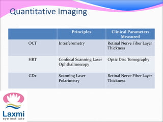
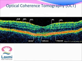
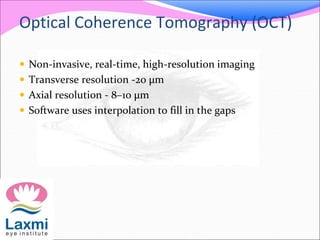
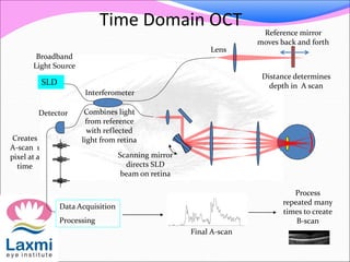
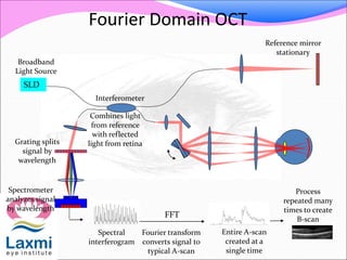
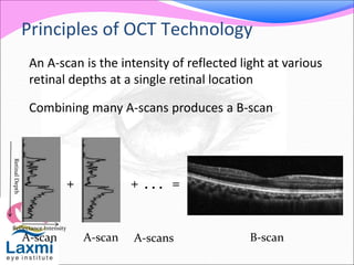
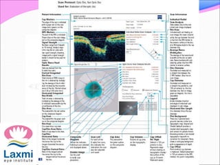
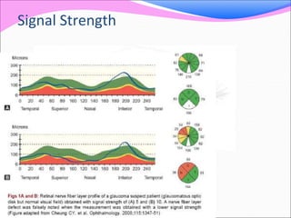
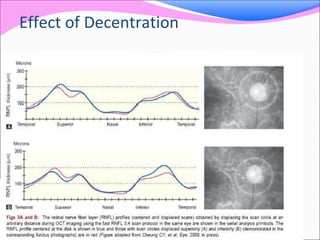
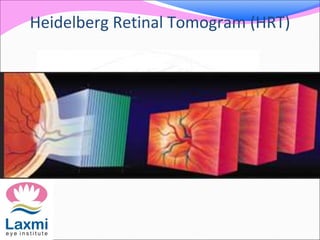
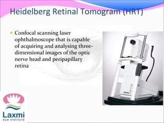
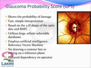
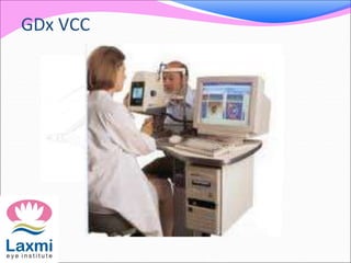
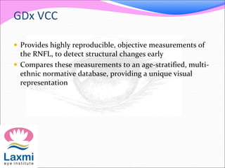
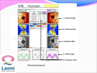
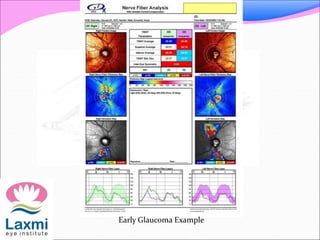
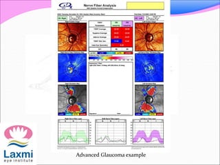
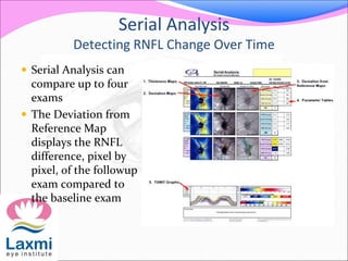
This document discusses various imaging techniques used to evaluate glaucoma, including OCT, HRT, and GDx. OCT uses interferometry to measure retinal nerve fiber layer thickness. HRT uses confocal laser scanning to create 3D images of the optic nerve and measure disc parameters. GDx uses scanning laser polarimetry to measure retinal nerve fiber layer thickness and detect glaucomatous damage through thickness maps, deviation maps, and TSNIT plots compared to normative data. Together these quantitative imaging techniques provide objective assessment to aid in glaucoma diagnosis and detection of progression.

1. IMAGING TECHNIQUES IN
GLAUCOMA
Presenter: Dr. Rujuta
Moderator: Dr. Rita Dhamankar

2. Various imaging techniques
 Anterior Segment:
 AS-OCT
 UBM
 Posterior Segment:
 OCT
 HRT
 GDx

3. Stereoscopic Optic Disc Photography
 Used to document structural abnormalities and
longitudinal changes in glaucomatous eyes
 Highly reproducible and records a natural color image of
the retina
 Conventional ONH evaluation includes estimation of the
ONH dimensions by observing the image pair with a
stereo viewer
 In the stereo image pair, depth is inversely proportional to
the disparity between the two matching points from the
left and right images

4. Quantitative Imaging
Principles Clinical Parameters
Measured
OCT Interferometry Retinal Nerve Fiber Layer
Thickness
HRT Confocal Scanning Laser
Ophthalmoscopy
Optic Disc Tomography
GDx Scanning Laser
Polarimetry
Retinal Nerve Fiber Layer
Thickness

5. Optical Coherence Tomography (OCT)

6. Optical Coherence Tomography (OCT)
 Non-invasive, real-time, high-resolution imaging
 Transverse resolution -20 μm
 Axial resolution - 8–10 μm
 Software uses interpolation to fill in the gaps

7. Optical Coherence Tomography (OCT)
 OCT uses a principle called low coherence interferometry
to derive depth information of various retinal structures
 This is performed by comparing the time difference in
reflected light from the retina at various depths with a
reference ‘standard’
 Differences between the reflected light and the reference
standard provide structural information in the form of an
‘A’ scan

8. Time Domain OCT
SLD
Lens
Detector
Data Acquisition
Processing
Combines light
from reference
with reflected
light from retina
Distance determines
depth in A scan
Reference mirror
moves back and forth
Scanning mirror
directs SLD
beam on retina
Interferometer
Broadband
Light Source
Creates
A-scan 1
pixel at a
time
Final A-scan
Process
repeated many
times to create
B-scan

9. Fourier Domain OCT
SLD
Spectrometer
analyzes signal
by wavelength
FFT
Grating splits
signal by
wavelength
Broadband
Light Source
Reference mirror
stationary
Combines light
from reference
with reflected
light from retina
Interferometer
Spectral
interferogram
Fourier transform
converts signal to
typical A-scan
Entire A-scan
created at a
single time
Process
repeated many
times to create
B-scan

10. Principles of OCT Technology
An A-scan is the intensity of reflected light at various
retinal depths at a single retinal location
Combining many A-scans produces a B-scan
A-scan A-scan
+ + . . . =
B-scanA-scans
RetinalDepth
Reflectance Intensity

11. RNFL Analysis
 Analysis of RNFL aids in identification of early
glaucomatous loss
 Circular scans of 3.4 mm diameter in the peripapillary
region (cylindrical retinal cross-section)
 RNFL thickness measurement is graphed in a TSNIT
orientation
 Compared to age-matched normative data

12. Optic Nerve Head Analysis
 Radial line scans through optic disc provide crosssectional
information on cupping and neuroretinal rim area
 Disc margins are objectively identified using signal from
end of RPE
 Parameters:
 Disc
 cup and rim area
 horizontal and vertical cup-to-disc ratio
 vertical integrated rim area
 horizontal integrated rim width

16. Signal Strength

17. Signal Strength

18. Effect of Decentration

19. Heidelberg Retinal Tomogram (HRT)

20. Heidelberg Retinal Tomogram (HRT)
 Confocal scanning laser
ophthalmoscope that is capable
of acquiring and analysing three-
dimensional images of the optic
nerve head and peripapillary
retina

21. Confocal Scanning Laser Ophthalmoscopy
 Uses laser light instead of a bright flash of white light to
illuminate the retina
 Confocal imaging is the process of scanning an object
point by point by a focused laser beam and then capturing
the reflected light through a small aperture (a confocal
pinhole)
 The confocal pinhole suppresses light reflected or
scattered from outside of the focal plane, which otherwise
would blur the image. The result is a sharp, high contrast
image of the object layer located at the focal plane

22.  Advantages over Fundus Photography
 Improved image quality
 Small depth of focus
 Suppression of scattered light
 Patient comfort through less bright light
 3D imaging capability
 Video capability
 Effective imaging of patients who do not dilate well
Confocal Scanning Laser Ophthalmoscopy

23. Principle
 Rapid scanning 670-nm diode laser
 Emitted beam is redirected in the
x and y-axis
 Along a plane of focus perpendicular to z-axis using two
oscillating mirrors
 Two-dimensional image reflected from the surface of the
retina and optic disc
 The confocal aperture limits the depth from which reflected
light reaches the detector
 Confocal aperture is shifted to acquire multiple optical
sections through the tissue of interest in order to create a
layered three-dimensional image

24. What the HRT does
 Once the patient is positioned, HRT II automatically performs a
pre-scan through the optic disc to determine the depth of the
individual’s optic nerve.
 Using information from this pre-scan, the fine focus and scan
depth are automatically adjusted to ensure that the entire optic
disc is included on the imaging cross-sections.
 Next, it determines the number of imaging planes to use (range
of scan depth 1-4mm)
 Each successive scan plane is set to measure 0.0625 mm deeper
 Automatically obtains three scans for analysis.
 Aligns and averages the scans to create the mean topography
image

25. HRT Images
 Reflectance Image
 False-color image that appears similar
to a photograph of the optic disc
 Darker areas are regions of decreased
overall reflectance, whereas lighter
areas, such as the base of the cup, are
areas of the greatest reflectance
 Valuable in locating and drawing the
contour line around the disc margin

26. HRT Images
 Topographic Image
 Relays information concerning the
height of the surface contour of the
optic disc and retina
 False-color coded
 Pixels that appear bright in the
topographic image are deeper, and
dark pixels are elevated
 Thus, the neuroretinal rim should
appear darker than the surrounding
retina and the base of the cup usually
appears lightest

27. Analysis
 After the contour line is drawn around the border of the optic
disc, the software automatically places a reference plane parallel
to the peripapillary retinal surface located 50 μm below the
retinal surface
 The reference plane is used to calculate the thickness and cross-
sectional area of the retinal nerve fiber layer

28.  The parameters of area and volume of the neuroretinal rim and
optic cup are also calculated based on the location of the
reference plane. The cup is considered to be the area of the
image that falls below the reference plane, whereas areas that
are of greater height than the reference plane are considered the
neuroretinal rim

29. HRT can differentiate between normal & early
glaucomatous eyes with a sensitivity of 79% to 87% &
specificity of 84 to 90%

31. Moorfields Regression Analysis (MRA)
 MRA differentiates between
glaucomatous and healthy ONHs by
detecting diffuse and focal changes of the
neuroretinal rim area
 Encorporates ONH size, and the effect of
age
 Classifies the eye using normative data,
for both global and sectoral analyses, the
latter using six sectors
 Results are indicated as color-coded
symbols: A green checkmark when “inside
normal limits”; a yellow exclamation mark
when “borderline”; and a red cross when
“outside normal limits”.

33. Glaucoma Probability Score (GPS)
 Shows the probability of damage
 Fast, simple interpretation
 Based on the 3-D shape of the optic
disc and RNFL
 Utilizes large, ethnic-selectable
databases
 Employs artificial intelligence:
Relevance Vector Machine
 No drawing a contour line or
relying on a reference plane
 Reduced dependency on operator
skill

34. Topographic Change Analysis (TCA)
 Statistically-based progression algorithm that accurately
detects structural change over time by comparing
variability between examinations and providing a
statistical indicator of change
 Aligns subsequent images with the baseline examination,
providing a point-by-point analysis of the optic disc and
peripapillary RNFL

35. GDx VCC

36. GDx VCC
 Provides highly reproducible, objective measurements of
the RNFL, to detect structural changes early
 Compares these measurements to an age-stratified, multi-
ethnic normative database, providing a unique visual
representation

37. Scanning laser polarimetry
 Use of polarised light to measure the thickness of the
retinal nerve fiber layer
 Measures the phase shift (retardation) of polarized laser
light passing through the eye
 The phase of the light is changed by the arrangement and
density of retinal nerve fiber layer (RNFL)

38. Scanning laser polarimetry Principle
 The polarised laser scans the fundus, building a monochromatic
image
 The state of polarisation of the light is changed (retardation) as
it passes through birefringent tissue (cornea and RNFL)
 Corneal birefringence is eliminated (in part) by a proprietary
'corneal compensator‘
 The amount of retardation of light reflected from the fundus is
converted to RFNL thickness

39. GDx VCC
 Provides quantitative RNFL evaluation
 Key elements:
 Thickness Map
 Deviation Map
 TSNIT graph
 Parameter Table

40. Key Features of the Printout
 Fundus Image
 Useful for checking image quality
 Well focused
 Evenly illuminated
 Optic disc well centered

41. Key Features of the Printout
 Thickness Map
 Shows the RNFL thickness in a color-coded format
 Thick RNFL values are coloured yellow, orange, red
 Thin RNFL values are coloured dark blue, light blue, green

42. Key Features of the Printout
 Deviation Map
 Reveals the location and magnitude of RNFL defects over
the entire thickness map
 Analyzes a region 20° x 20° centered on the optic disc
 For each scan, the RNFL thickness at each pixel is
compared to the age-matched normative database, and
the pixels that fall below the normal range are flagged by
coloured squares based on the probability

43. Deviation Map continued…
 Dark blue squares represent areas
where the RNFL thickness is below
the 5th percentile of the normative
database
 Light blue squares represent deviation
below the 2% level
 Yellow represents deviation below 1%
 Red represents deviation below 0.05%
 Uses a grayscale fundus image of the
eye as a background

44. Deviation Maps for eyes at different stages of disease

45. Key Features of the Printout
 TSNIT Map
 Displayed at the bottom of the
printout
 In a normal eye the TSNIT plot
follows the typical ‘double hump’
pattern
 When there is RNFL loss, the TSNIT curve will fall below
this shaded area, especially in the superior and inferior
regions
 Also, a dip in the curve of one eye relative to another is
indicative of RNFL loss

46. Key Features of the Printout
 Parameter Table
 The TSNIT parameters are summary measures based on
RNFL thickness values within the calculation circle

47. Parameters continued…
 Inter-eye Symmetry: Measures the degree of symmetry
between the right and left eyes by correlating the TSNIT
functions from the two eyes
 Values range from –1 to 1, where values near one represent
good symmetry

48. The Nerve Fiber Indicator (NFI)
 Global measure based on the entire RNFL thickness map
 Calculated using an advanced form of neural network,
called a Support Vector Machine (SVM)
 Output values range from 1 –100
 1-30 -> normal
 31-50 -> borderline
 51+ -> abnormal

49. Normal printout

50. Early Glaucoma Example

51. Advanced Glaucoma example

52. Serial Analysis
Detecting RNFL Change Over Time
 Serial Analysis can
compare up to four
exams
 The Deviation from
Reference Map
displays the RNFL
difference, pixel by
pixel, of the followup
exam compared to
the baseline exam

53. Summary
 The imaging techniques provide comprehensive RNFL
assessment to aid the clinician in the diagnosis of
glaucoma
 However, they do not replace a careful clinical
evaluation or visual field testing