The document discusses image restoration and reconstruction techniques. It covers various topics: 1. Noise models and their probability density functions such as Gaussian, Rayleigh, Erlang, exponential, uniform, and impulse noise. 2. Spatial filtering techniques for noise removal including mean filtering, order-statistics filters like median filtering, and adaptive filters. 3. Periodic noise reduction using frequency domain filtering methods such as bandreject filtering, bandpass filtering, and notch filtering. Code examples and results are provided for mean filtering, order-statistics filtering, and adaptive filtering applied to sample noisy images.

1. Topic:
Image Restoration and Reconstruction
Presenters:
Sadia Zafar (170403)
Mahnoor Fatima (170399)
Muhammad Usama (170355)

2. Image Restoration and Reconstruction
 Noise Models,
- Spatial + frequency properties of noise,
- Noise Probability Density functions,
- Periodic Noise.
 Restoration of Noise-Spatial Filtering,
- Mean Filtering,
- Order-Statistics Filters,
- Adaptive filters,
 Periodic Noise Reduction -Frequency
Filtering,
- Bandreject Filtering,
- Bandpass Filters,
- Notch filters,
 Inverse filtering,
 Wiener filtering,
Geometric Mean filtering,

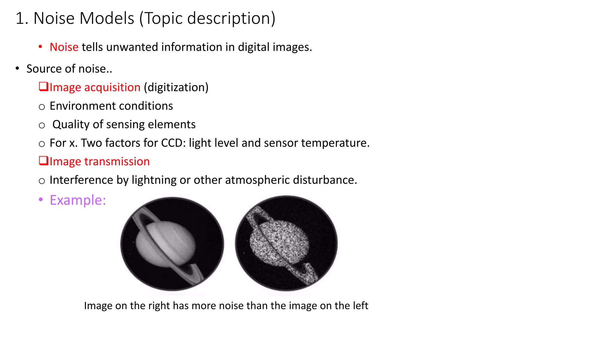
3. 1. Noise Models (Topic description)
• Noise tells unwanted information in digital images.
• Source of noise..
Image acquisition (digitization)
o Environment conditions
o Quality of sensing elements
o For x. Two factors for CCD: light level and sensor temperature.
Image transmission
o Interference by lightning or other atmospheric disturbance.
• Example:
Image on the right has more noise than the image on the left

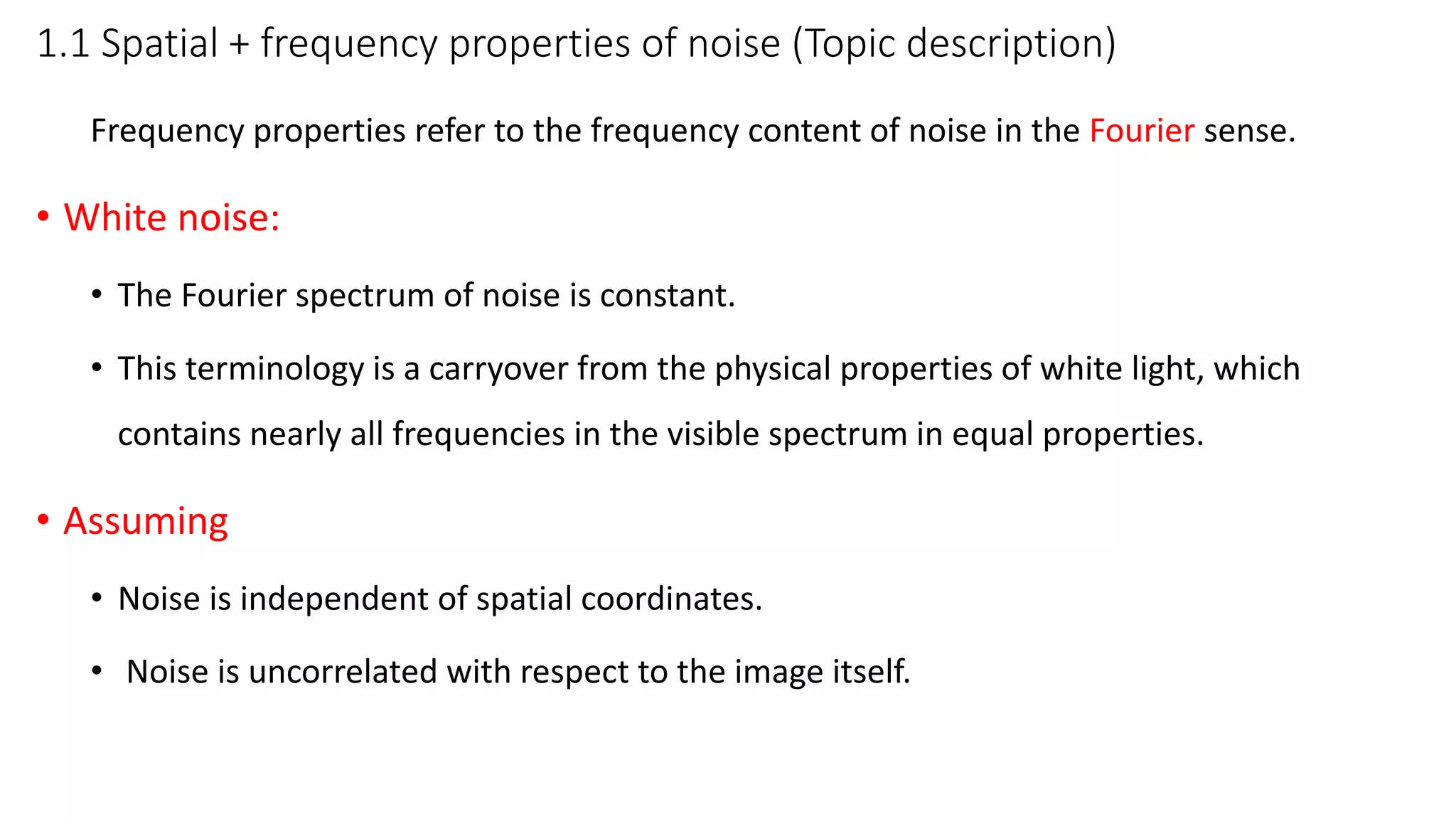
4. 1.1 Spatial + frequency properties of noise (Topic description)
Frequency properties refer to the frequency content of noise in the Fourier sense.
• White noise:
• The Fourier spectrum of noise is constant.
• This terminology is a carryover from the physical properties of white light, which
contains nearly all frequencies in the visible spectrum in equal properties.
• Assuming
• Noise is independent of spatial coordinates.
• Noise is uncorrelated with respect to the image itself.

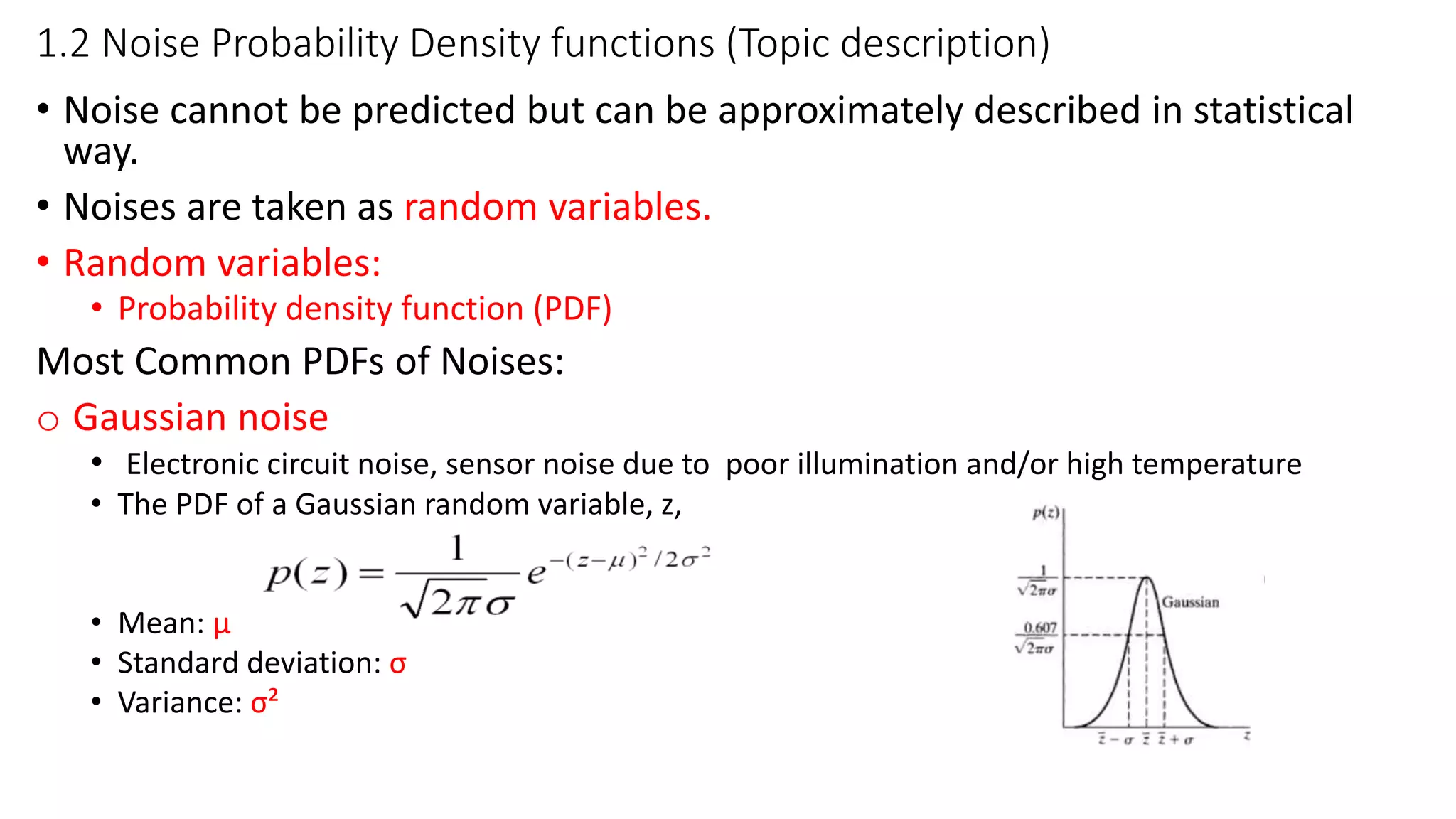
5. 1.2 Noise Probability Density functions (Topic description)
• Noise cannot be predicted but can be approximately described in statistical
way.
• Noises are taken as random variables.
• Random variables:
• Probability density function (PDF)
Most Common PDFs of Noises:
o Gaussian noise
• Electronic circuit noise, sensor noise due to poor illumination and/or high temperature
• The PDF of a Gaussian random variable, z,
• Mean: µ
• Standard deviation: σ
• Variance: σ²

6. 1.2 Noise Probability Density functions (Cont.)
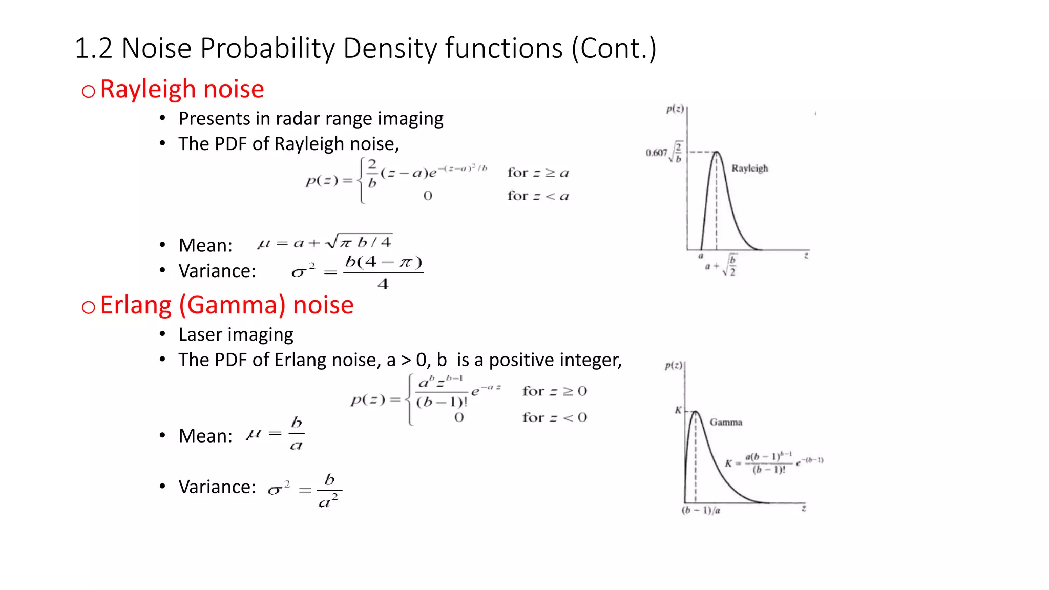
oRayleigh noise
• Presents in radar range imaging
• The PDF of Rayleigh noise,
• Mean:
• Variance:
oErlang (Gamma) noise
• Laser imaging
• The PDF of Erlang noise, a > 0, b is a positive integer,
• Mean:
• Variance:

7. 1.2 Noise Probability Density functions (Cont.)
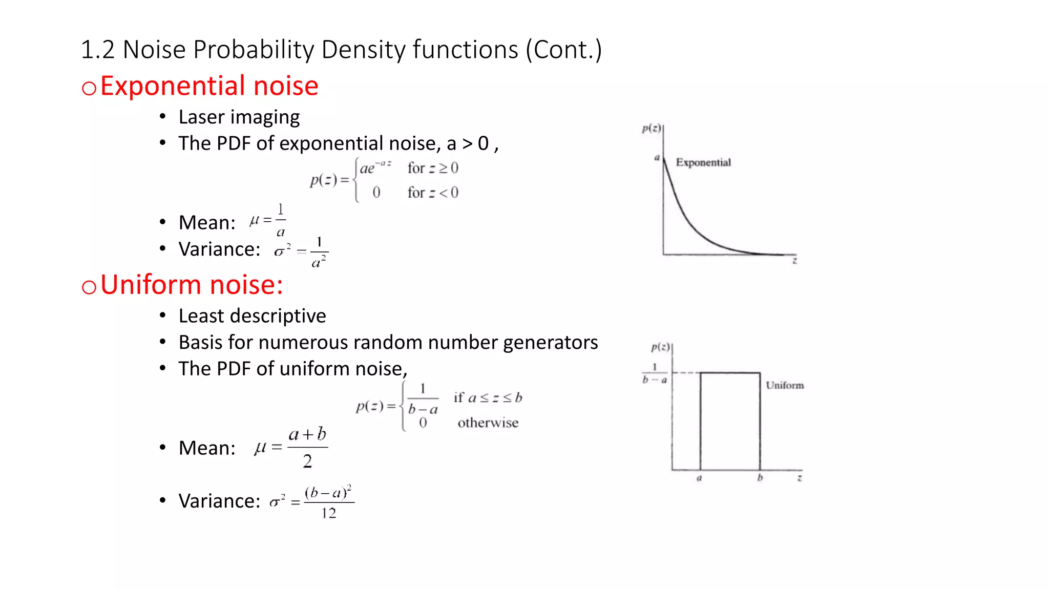
oExponential noise
• Laser imaging
• The PDF of exponential noise, a > 0 ,
• Mean:
• Variance:
oUniform noise:
• Least descriptive
• Basis for numerous random number generators
• The PDF of uniform noise,
• Mean:
• Variance:

8. 1.2 Noise Probability Density functions (Cont.)
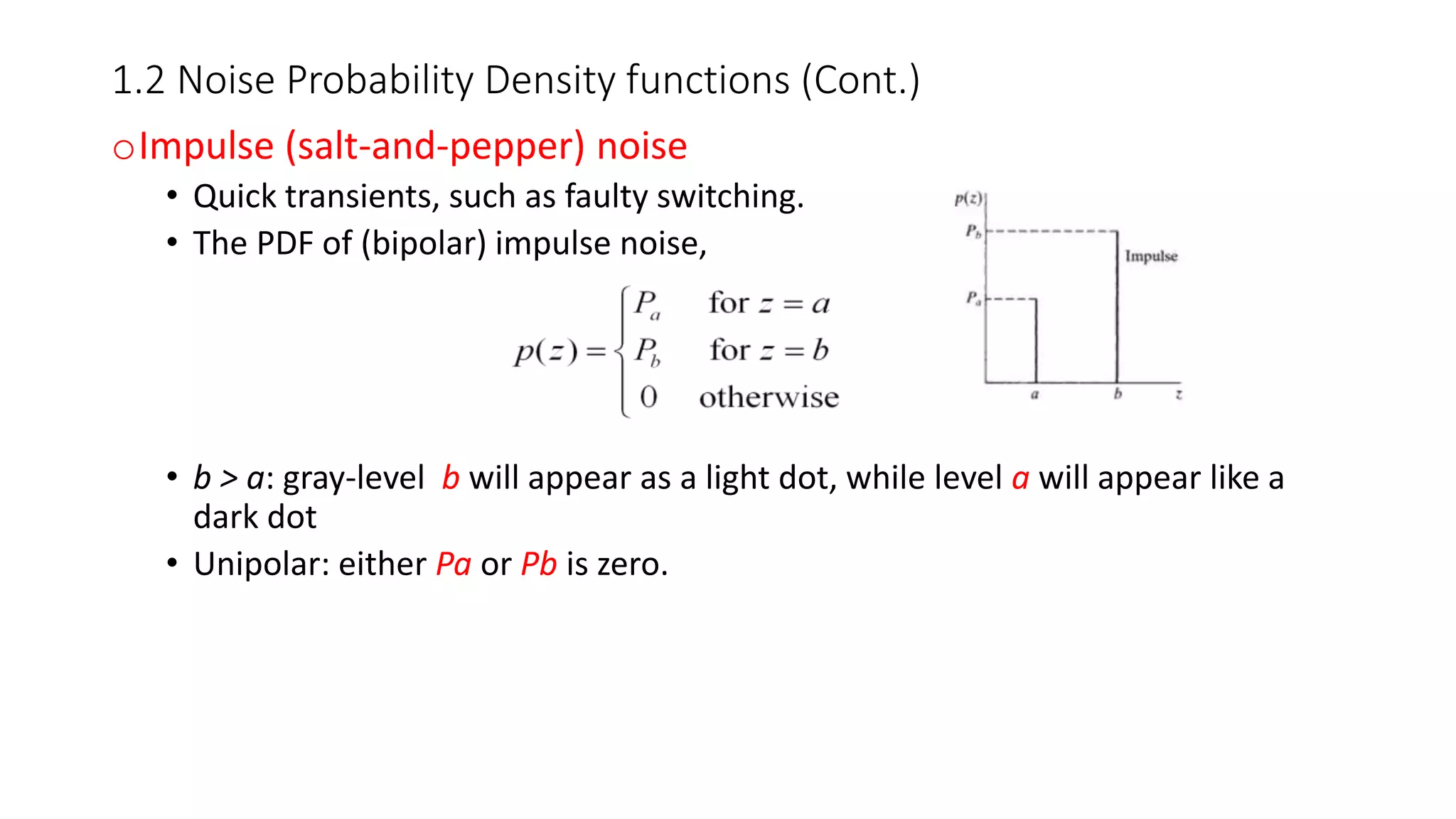
oImpulse (salt-and-pepper) noise
• Quick transients, such as faulty switching.
• The PDF of (bipolar) impulse noise,
• b > a: gray-level b will appear as a light dot, while level a will appear like a
dark dot
• Unipolar: either Pa or Pb is zero.

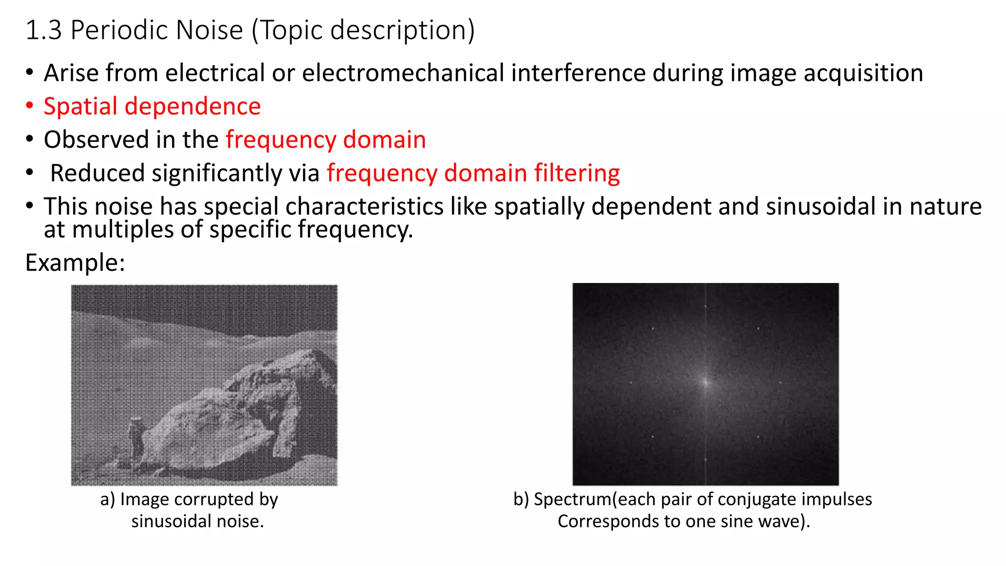
9. 1.3 Periodic Noise (Topic description)
• Arise from electrical or electromechanical interference during image acquisition
• Spatial dependence
• Observed in the frequency domain
• Reduced significantly via frequency domain filtering
• This noise has special characteristics like spatially dependent and sinusoidal in nature
at multiples of specific frequency.
Example:
a) Image corrupted by b) Spectrum(each pair of conjugate impulses
sinusoidal noise. Corresponds to one sine wave).

10. Implemented Code :
a = imread('Desktopnoise.jpg');
a = imresize(a, [256 256],'nearest');
subplot(2,3,1);
imshow(a);
title('Original Image');
%Adding Salt and pepper noise
b = imnoise(a, 'salt & pepper',0.02);
subplot(2,3,2);
imshow(b);
title('Salt & Pepper Image');
%Adding gaussian noise
c = imnoise(a,'gaussian',0,0.01);
subplot(2,3,3);
imshow(c);
title('Gaussian Image');
1. Noise Models (Hands-on Practices-Hour)
Implemented Results :

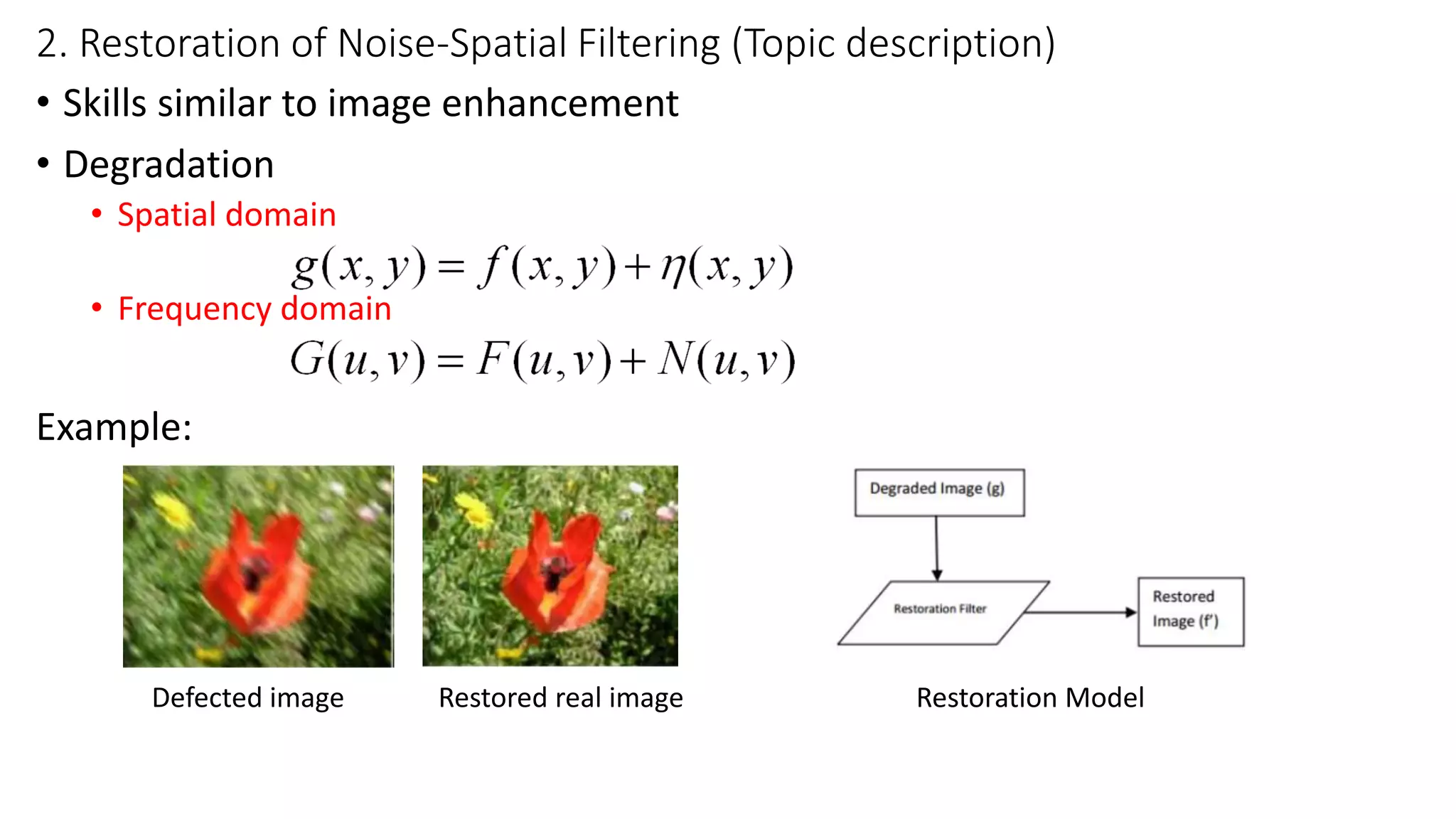
11. 2. Restoration of Noise-Spatial Filtering (Topic description)
• Skills similar to image enhancement
• Degradation
• Spatial domain
• Frequency domain
Example:
Defected image Restored real image Restoration Model

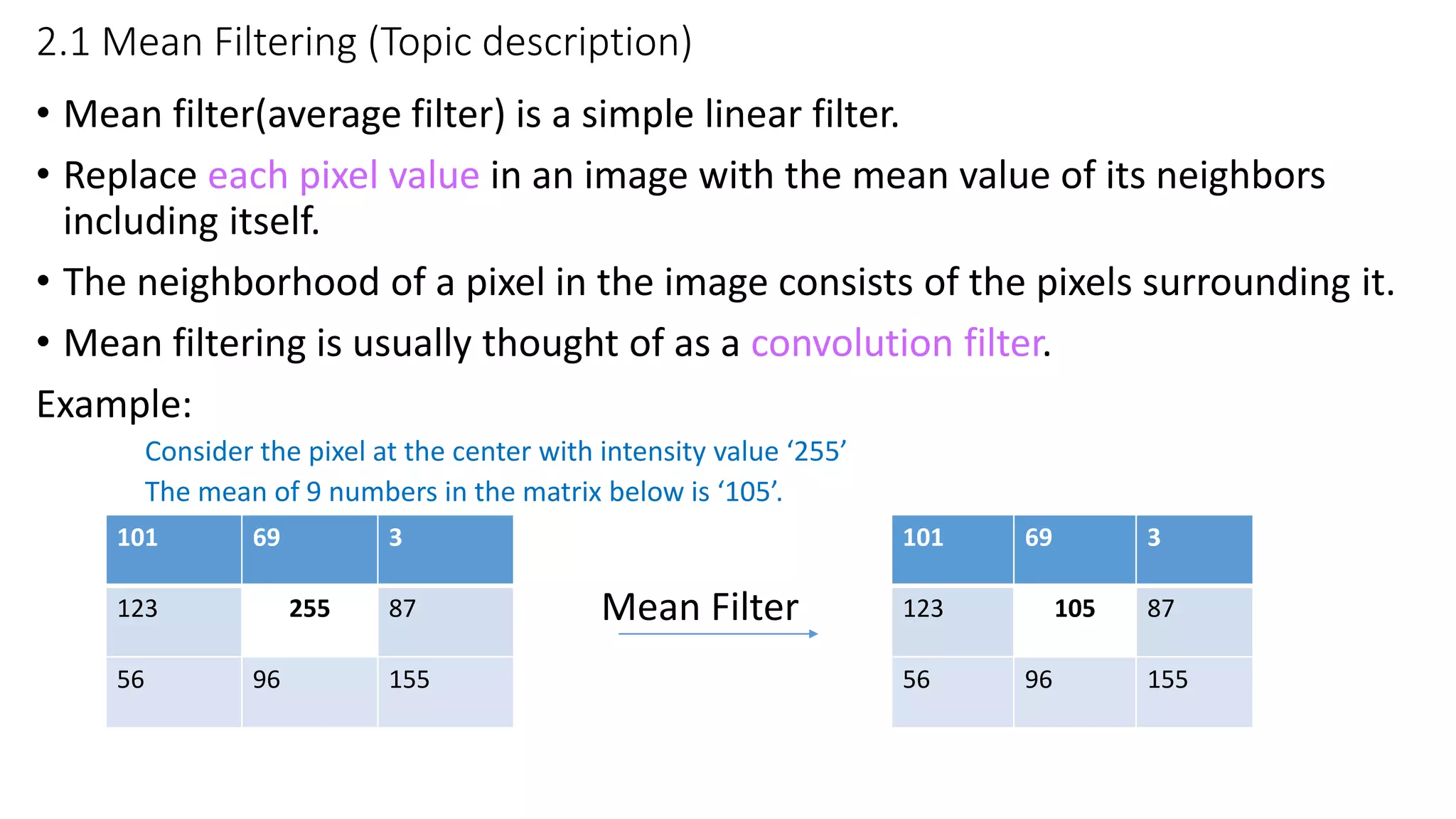
12. 2.1 Mean Filtering (Topic description)
• Mean filter(average filter) is a simple linear filter.
• Replace each pixel value in an image with the mean value of its neighbors
including itself.
• The neighborhood of a pixel in the image consists of the pixels surrounding it.
• Mean filtering is usually thought of as a convolution filter.
Example:
Consider the pixel at the center with intensity value ‘255’
The mean of 9 numbers in the matrix below is ‘105’.
Mean Filter
101 69 3
123 255 87
56 96 155
101 69 3
123 105 87
56 96 155

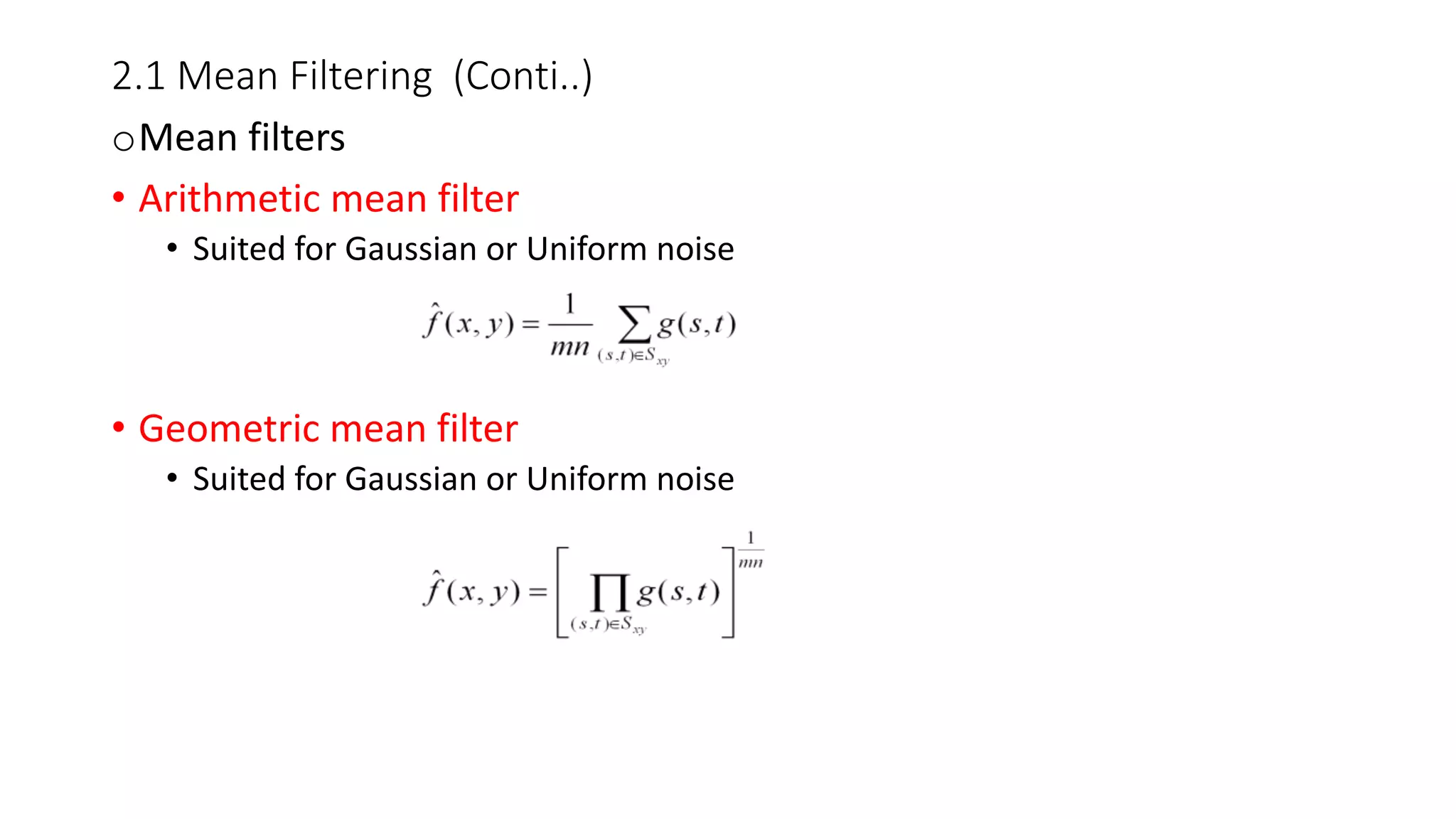
13. 2.1 Mean Filtering (Conti..)
oMean filters
• Arithmetic mean filter
• Suited for Gaussian or Uniform noise
• Geometric mean filter
• Suited for Gaussian or Uniform noise

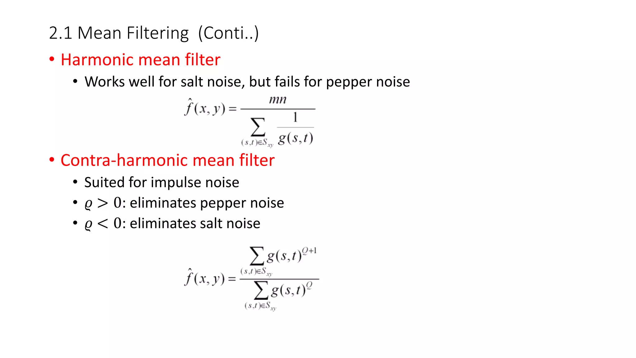
14. 2.1 Mean Filtering (Conti..)
• Harmonic mean filter
• Works well for salt noise, but fails for pepper noise
• Contra-harmonic mean filter
• Suited for impulse noise
• 𝜚 > 0: eliminates pepper noise
• 𝜚 < 0: eliminates salt noise

15. 2.2 Order-Statistics Filters (Topic description)
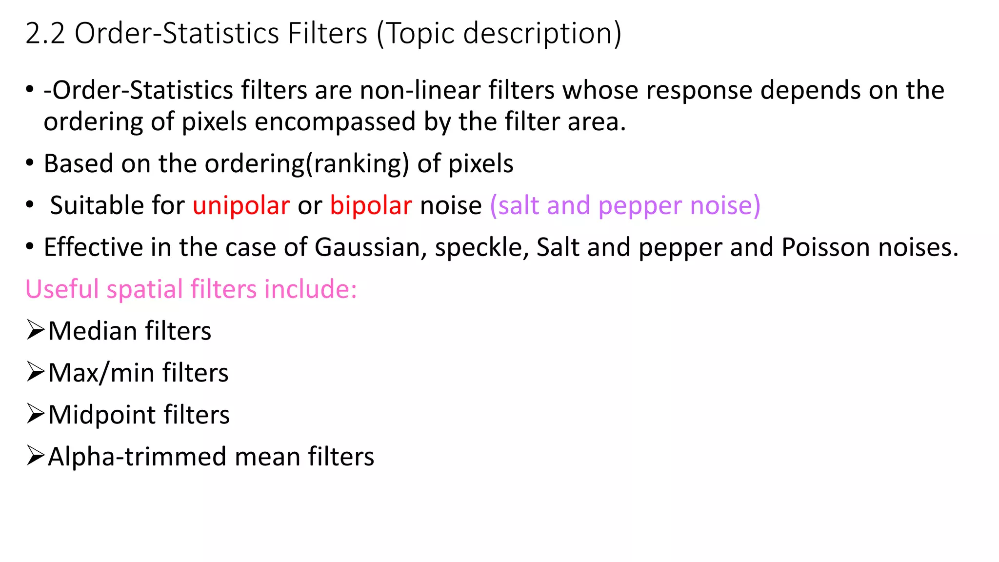
• -Order-Statistics filters are non-linear filters whose response depends on the
ordering of pixels encompassed by the filter area.
• Based on the ordering(ranking) of pixels
• Suitable for unipolar or bipolar noise (salt and pepper noise)
• Effective in the case of Gaussian, speckle, Salt and pepper and Poisson noises.
Useful spatial filters include:
Median filters
Max/min filters
Midpoint filters
Alpha-trimmed mean filters

16. 2.2 Order-Statistics Filters (Conti..)
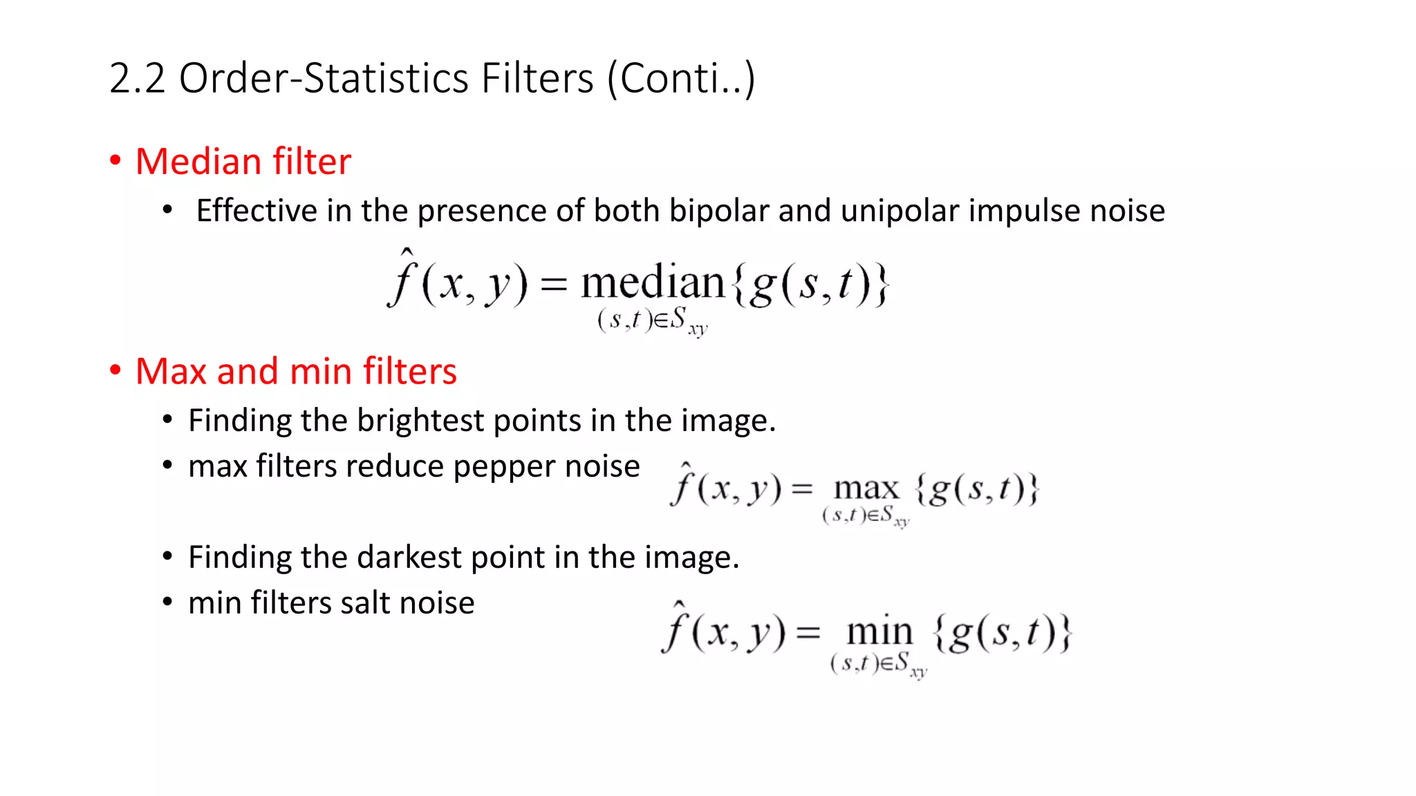
• Median filter
• Effective in the presence of both bipolar and unipolar impulse noise
• Max and min filters
• Finding the brightest points in the image.
• max filters reduce pepper noise
• Finding the darkest point in the image.
• min filters salt noise

17. 2.2 Order-Statistics Filters (Conti..)
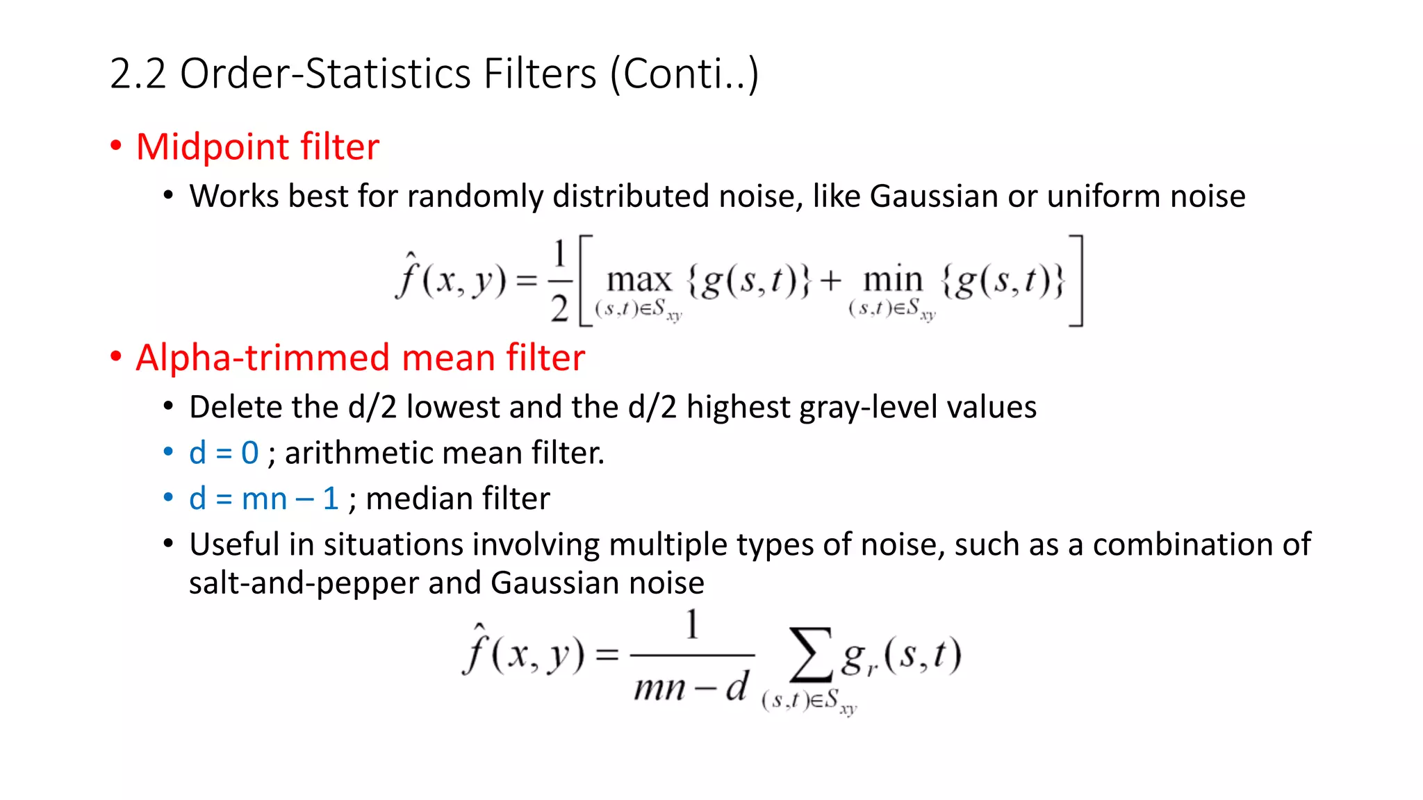
• Midpoint filter
• Works best for randomly distributed noise, like Gaussian or uniform noise
• Alpha-trimmed mean filter
• Delete the d/2 lowest and the d/2 highest gray-level values
• d = 0 ; arithmetic mean filter.
• d = mn – 1 ; median filter
• Useful in situations involving multiple types of noise, such as a combination of
salt-and-pepper and Gaussian noise

18. 2.3 Adaptive filters (Topic description)
• Adapted to the behavior based on the statistical characteristics of
the image inside the filter region Sxy defined by the m х n
rectangular window.
• An adaptive filter is one which can automatically design itself and
can detect system variation in time.
• The performance is superior to that of the filters discussed before.
• Improved performance vs increased complexity
• Example:
Adaptive local noise reduction filter

19. 2.3 Adaptive filters include: (Cont..)
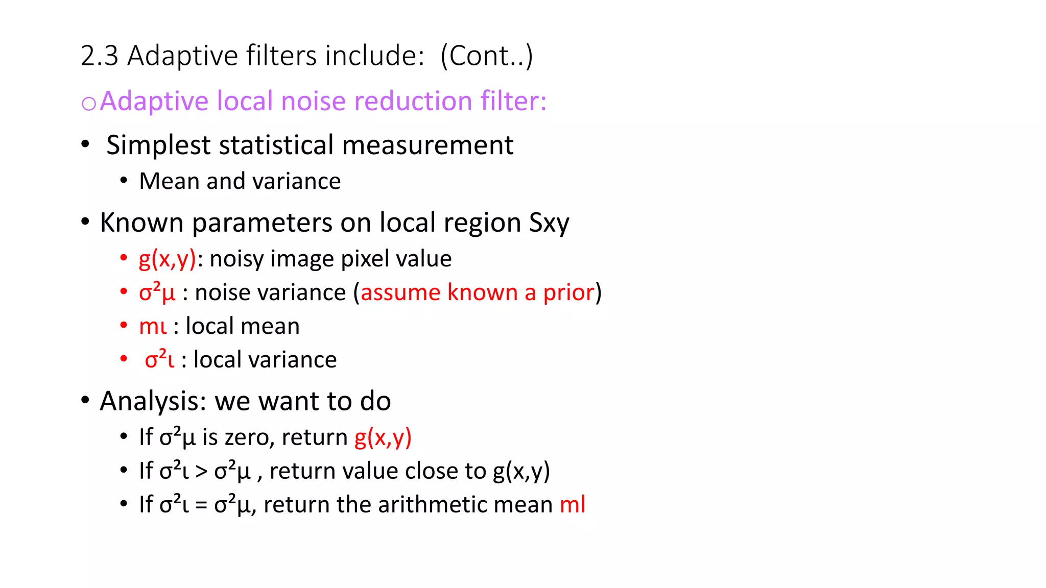
oAdaptive local noise reduction filter:
• Simplest statistical measurement
• Mean and variance
• Known parameters on local region Sxy
• g(x,y): noisy image pixel value
• σ²µ : noise variance (assume known a prior)
• mι : local mean
• σ²ι : local variance
• Analysis: we want to do
• If σ²µ is zero, return g(x,y)
• If σ²ι > σ²µ , return value close to g(x,y)
• If σ²ι = σ²µ, return the arithmetic mean ml

20. Implemented Code :
I = imread('DesktopDIP Projectlena.png');
Img = rgb2gray(I);
[m,n] = size(Img);
output = zeros(m,n);
for i=1:m
for j=1:n
rmin = max (1, i-1);
rmax = min(m, i+1);
cmin = max(1,j-1);
cmax = min(n,j+1);
temp = Img(rmin:rmax,cmin:cmax);
output(i,j) = mean(temp(:));
end
end
output = uint8(output);
figure(1);
set(gcf,'Position',get(0,'Screensize'));
subplot(121),imshow(Img),title('Original
Image');
subplot(122),imshow(output),title('Output of
Mean Filter’);
2. Mean Filtering (Hands-on Practices-Hour)
Implemented Results :

21. Implemented Code :
I = imread('cameraman.tif');
imshow(I);
subplot(121);
title('Order of pixel values')
rank = 2;
[a,b] = size(I);
c = zeros(a-2, b-2);
for i=1: a-2
for j=1: b-2
ss = sort(reshape(I(i:i+2,j:j+2),[1,9]));
c(i+1,j+1)=ss(rank);
end
end
figure(1)
subplot(122)
imshow(mat2gray(c))
title('Order Statics Filter Image');
2. Order-Statistics Filters (Hands-on Practices-Hour)
Implemented Results :

22. Implemented Code :
Im = imread('DesktopDIP Projectnoise.jpg');
I = rgb2gray(Im);
[rows, columns, numberOfColorBands]=size(I);
subplot(1,3,1);
imshow(I);
title ('Original Image');
n = imnoise(I, 'salt & pepper' , 0.05);
subplot(1,3,2);
imshow(n);
title('Salt & Pepper Noise');
m = medfilt2(n,[7 7]);
noiseImage = (n == 0 | n == 255);
I_nf = n;
I_nf(noiseImage) = m(noiseImage);
subplot(1,3,3);
imshow(I_nf);
title('Median Filter');
2. Adaptive filters (Hands-on Practices-Hour)
Implemented Results :

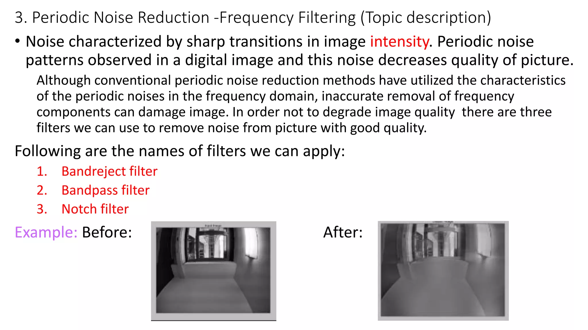
23. 3. Periodic Noise Reduction -Frequency Filtering (Topic description)
• Noise characterized by sharp transitions in image intensity. Periodic noise
patterns observed in a digital image and this noise decreases quality of picture.
Although conventional periodic noise reduction methods have utilized the characteristics
of the periodic noises in the frequency domain, inaccurate removal of frequency
components can damage image. In order not to degrade image quality there are three
filters we can use to remove noise from picture with good quality.
Following are the names of filters we can apply:
1. Bandreject filter
2. Bandpass filter
3. Notch filter
Example: Before: After:

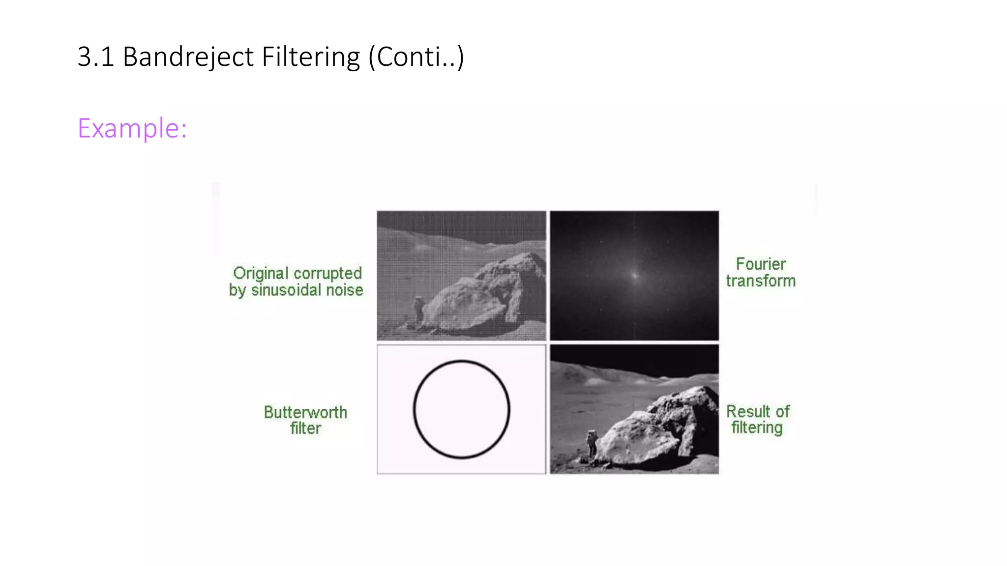
24. 3.1 Bandreject Filtering (Topic description)
Fundamental principle application of bandreject filter is Removing periodic
noise from an image involves a particular range of frequencies from that image.
• It is also known as band-stop filter.
• It overpower frequency content within a range between a lower and higher
cut off frequency.
• There are three versions of Bandreject filter
I. Ideal bandreject filter.
II. Gaussian bandreject filter.
III. Butterworth bandreject filter.

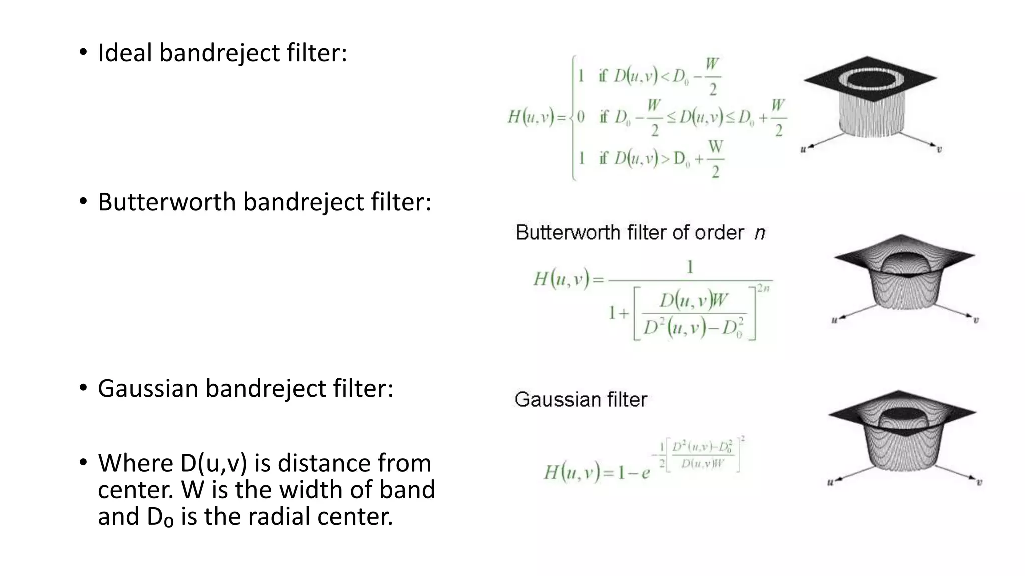
25. • Ideal bandreject filter:
• Butterworth bandreject filter:
• Gaussian bandreject filter:
• Where D(u,v) is distance from
center. W is the width of band
and D₀ is the radial center.

26. 3.1 Bandreject Filtering (Conti..)
Example:

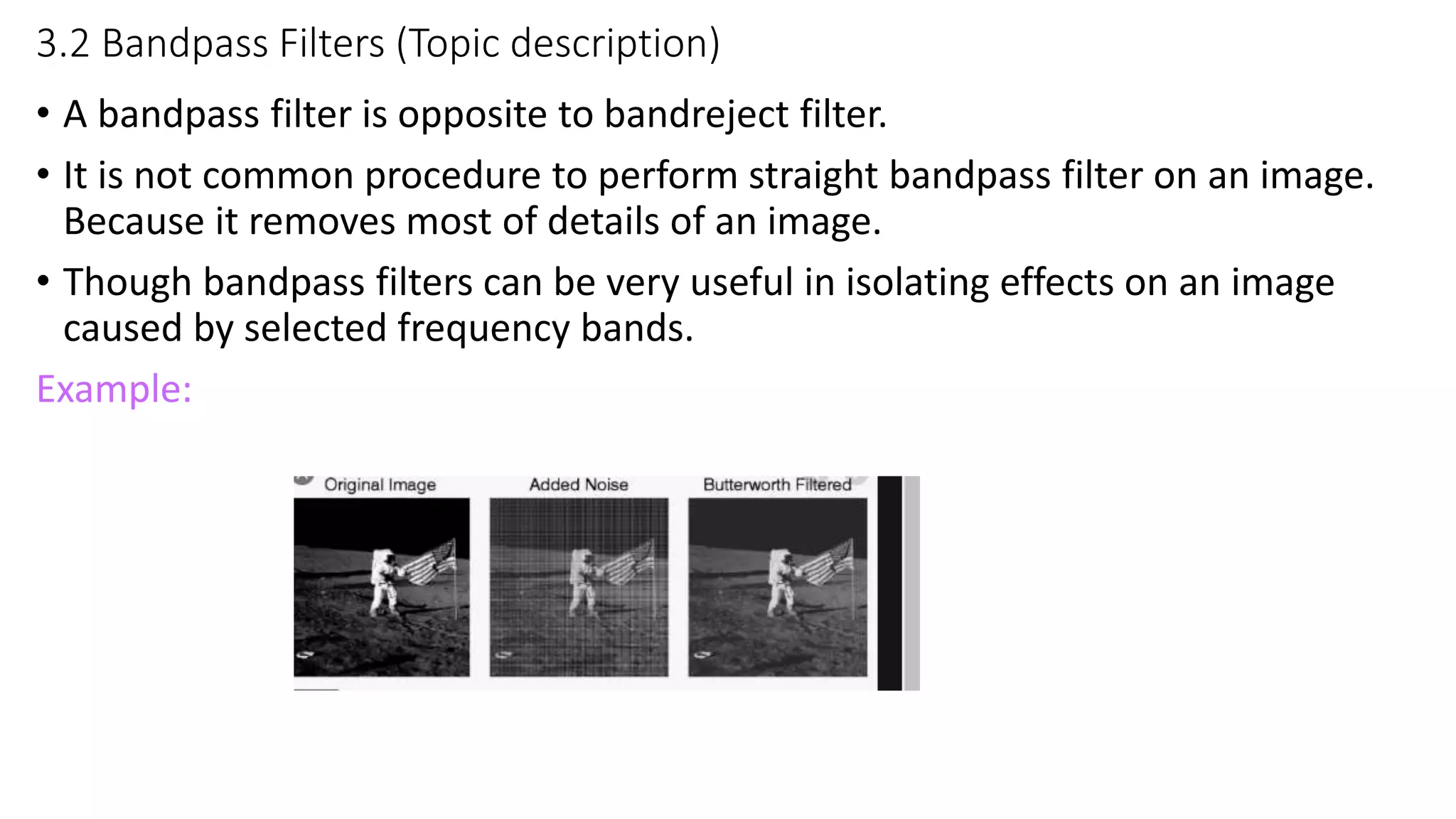
27. 3.2 Bandpass Filters (Topic description)
• A bandpass filter is opposite to bandreject filter.
• It is not common procedure to perform straight bandpass filter on an image.
Because it removes most of details of an image.
• Though bandpass filters can be very useful in isolating effects on an image
caused by selected frequency bands.
Example:

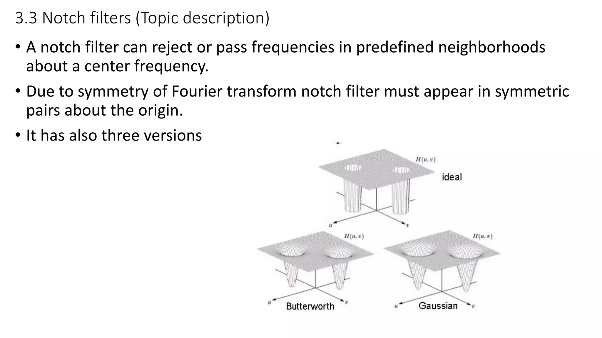
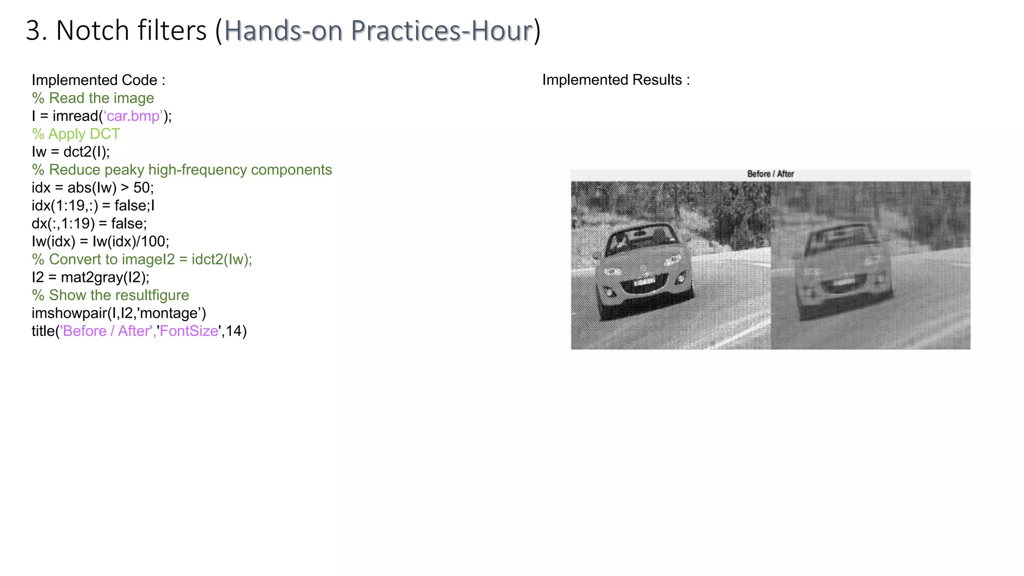
28. 3.3 Notch filters (Topic description)
• A notch filter can reject or pass frequencies in predefined neighborhoods
about a center frequency.
• Due to symmetry of Fourier transform notch filter must appear in symmetric
pairs about the origin.
• It has also three versions

29. 3.3 Notch filters (Cont..)
• Notch filters versions:

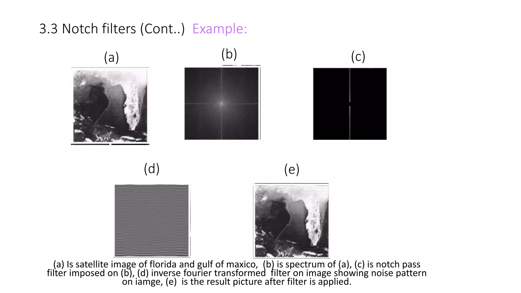
30. (a) Is satellite image of florida and gulf of maxico, (b) is spectrum of (a), (c) is notch pass
filter imposed on (b), (d) inverse fourier transformed filter on image showing noise pattern
on iamge, (e) is the result picture after filter is applied.
3.3 Notch filters (Cont..) Example:
(a)
(e)
(c)(b)
(d)

31. Implemented Code :
im = imread('H:cde.jpg')
figure,imshow(im)
FT = fft2(double(im));
FT1 = fftshift(FT);
imtool(abs(FT1),[]);
m = size(im,1);
n =size(im,2);
t = 0:pi/20:2*pi;
xc = (m+150)/2;
yc = (n-150)/2;
r=200;
r1=40;
xcc=r*cos(t)+xc;
ycc=r*sin(t)+yc;
xcc1=r1*cos(t)+xc;
ycc1=r1*sin(t)+yc;
mask=poly2mask(double(xcc),double(ycc),m,n);
mask1=poly2mask(double(xcc),double(ycc),m,n);
mask=mask(1);
FT2=FT1;
FT2(mask)=0;
imtool(abs(FT2),[]);
output=ifft2(ifftshift(FT2));
imtool(output,[]);
3. Bandreject Filtering (Hands-on Practices-Hour)
Results :

32. Implemented Code :
rp=0.2;
rs=20;
fp=200;
fs=600;
f=2000;
wp=2*(fp/f);
ws=2*(fs/f);
[n,wn]=buttord(wp,ws,rp,rs);
Wn=[wp,ws];
[b,a]=butter(n,wn);
[h,w]=freqz(b,a);
Subplot(2,1,1);
Plot(w/pi,20*log(abs(h)));
Grid;Xlabel('nf’);
Ylabel('mag’);
title('mag response’);
Subplot(2,1,2);
Plot(w/pi,angle(h));
Grid;xlabel('nf’);
ylabel('angle’);
title('phase response');
3. Bandpass Filters (Hands-on Practices-Hour)
Implemented Results :

33. Implemented Code :
% Read the image
I = imread(‘car.bmp’);
% Apply DCT
Iw = dct2(I);
% Reduce peaky high-frequency components
idx = abs(Iw) > 50;
idx(1:19,:) = false;I
dx(:,1:19) = false;
Iw(idx) = Iw(idx)/100;
% Convert to imageI2 = idct2(Iw);
I2 = mat2gray(I2);
% Show the resultfigure
imshowpair(I,I2,'montage’)
title('Before / After','FontSize',14)
3. Notch filters (Hands-on Practices-Hour)
Implemented Results :

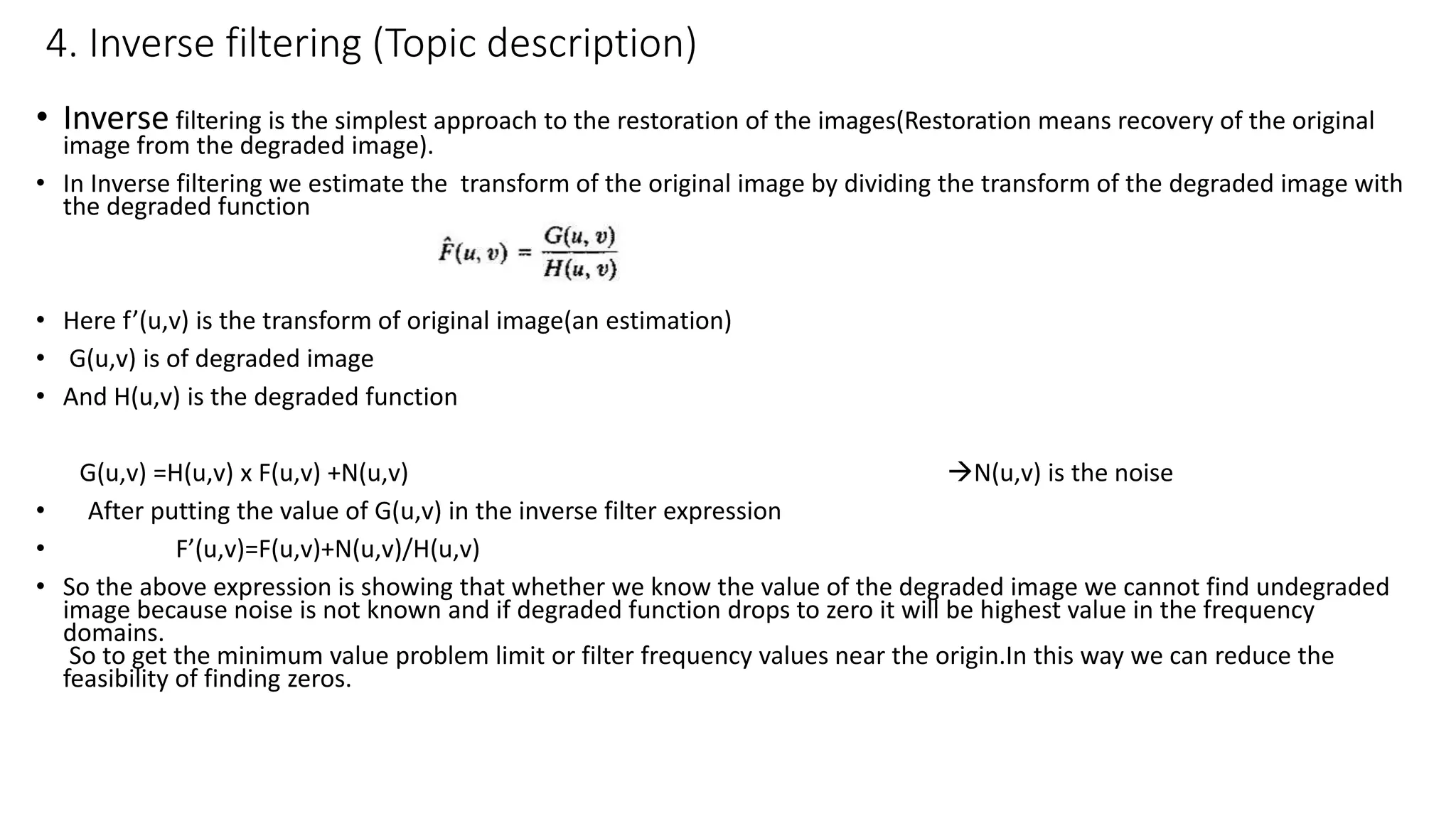
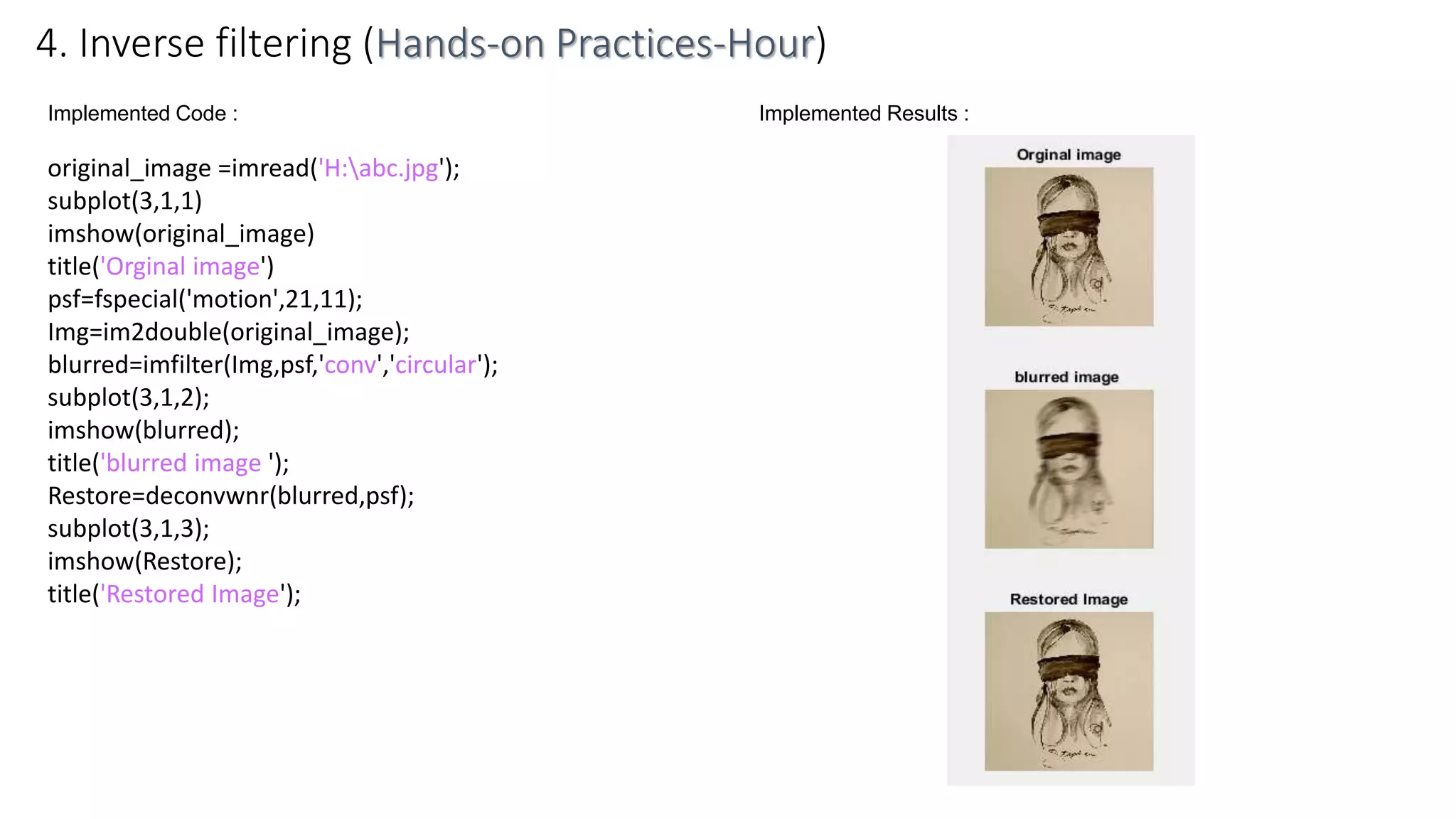
34. 4. Inverse filtering (Topic description)
• Inverse filtering is the simplest approach to the restoration of the images(Restoration means recovery of the original
image from the degraded image).
• In Inverse filtering we estimate the transform of the original image by dividing the transform of the degraded image with
the degraded function
• Here f’(u,v) is the transform of original image(an estimation)
• G(u,v) is of degraded image
• And H(u,v) is the degraded function
G(u,v) =H(u,v) x F(u,v) +N(u,v) N(u,v) is the noise
• After putting the value of G(u,v) in the inverse filter expression
• F’(u,v)=F(u,v)+N(u,v)/H(u,v)
• So the above expression is showing that whether we know the value of the degraded image we cannot find undegraded
image because noise is not known and if degraded function drops to zero it will be highest value in the frequency
domains.
So to get the minimum value problem limit or filter frequency values near the origin.In this way we can reduce the
feasibility of finding zeros.

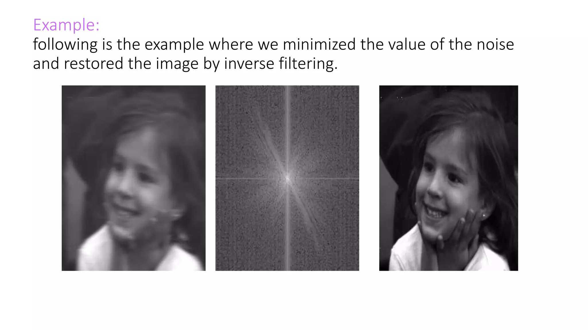
35. Example:
following is the example where we minimized the value of the noise
and restored the image by inverse filtering.

36. Implemented Code :
original_image =imread('H:abc.jpg');
subplot(3,1,1)
imshow(original_image)
title('Orginal image')
psf=fspecial('motion',21,11);
Img=im2double(original_image);
blurred=imfilter(Img,psf,'conv','circular');
subplot(3,1,2);
imshow(blurred);
title('blurred image ');
Restore=deconvwnr(blurred,psf);
subplot(3,1,3);
imshow(Restore);
title('Restored Image');
4. Inverse filtering (Hands-on Practices-Hour)
Implemented Results :

37. 5. Wiener filtering (Topic description)
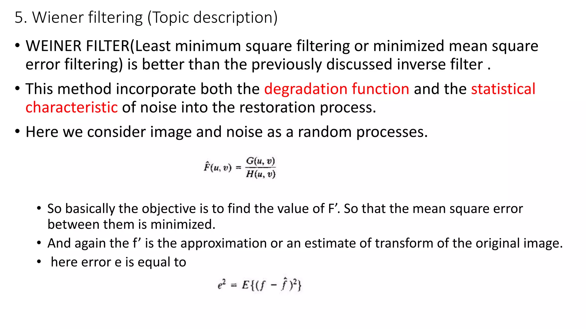
• WEINER FILTER(Least minimum square filtering or minimized mean square
error filtering) is better than the previously discussed inverse filter .
• This method incorporate both the degradation function and the statistical
characteristic of noise into the restoration process.
• Here we consider image and noise as a random processes.
• So basically the objective is to find the value of F’. So that the mean square error
between them is minimized.
• And again the f’ is the approximation or an estimate of transform of the original image.
• here error e is equal to

38. 5. Wiener filtering (Conti..)
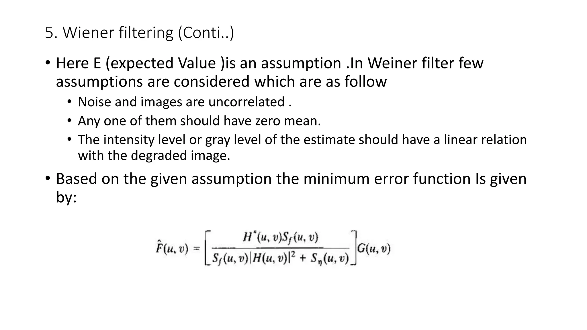
• Here E (expected Value )is an assumption .In Weiner filter few
assumptions are considered which are as follow
• Noise and images are uncorrelated .
• Any one of them should have zero mean.
• The intensity level or gray level of the estimate should have a linear relation
with the degraded image.
• Based on the given assumption the minimum error function Is given
by:

39. 5. Wiener filtering (Conti..)
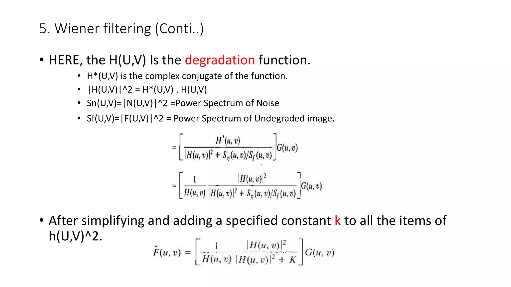
• HERE, the H(U,V) Is the degradation function.
• H*(U,V) is the complex conjugate of the function.
• |H(U,V)|^2 = H*(U,V) . H(U,V)
• Sn(U,V)=|N(U,V)|^2 =Power Spectrum of Noise
• Sf(U,V)=|F(U,V)|^2 = Power Spectrum of Undegraded image.
• After simplifying and adding a specified constant k to all the items of
h(U,V)^2.

40. Example : (Wiener filtering)

41. Implemented Code :
original =imread('H:abc.jpg');
i=rgb2gray(original);
j=imnoise(i,'Gaussian',0,0.0025);
imshow(j);
title('Gaussian Noise Added');
image=wiener2(j,[3 3]);
figure;
imshow(image);
title('Restored Image');
5. Wiener filtering (Hands-on Practices-Hour)
Implemented Results :

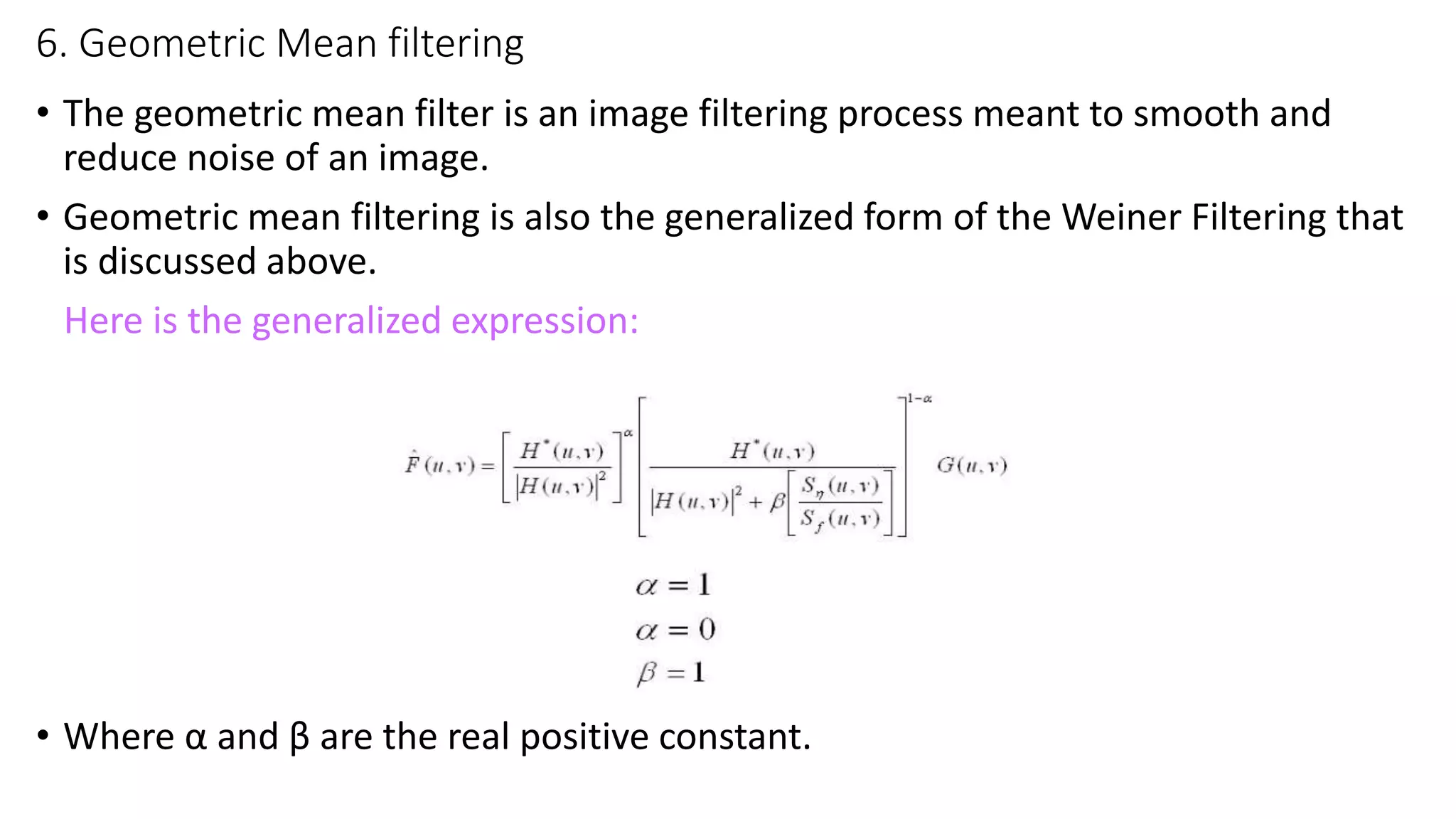
42. 6. Geometric Mean filtering
• The geometric mean filter is an image filtering process meant to smooth and
reduce noise of an image.
• Geometric mean filtering is also the generalized form of the Weiner Filtering that
is discussed above.
Here is the generalized expression:
• Where α and β are the real positive constant.

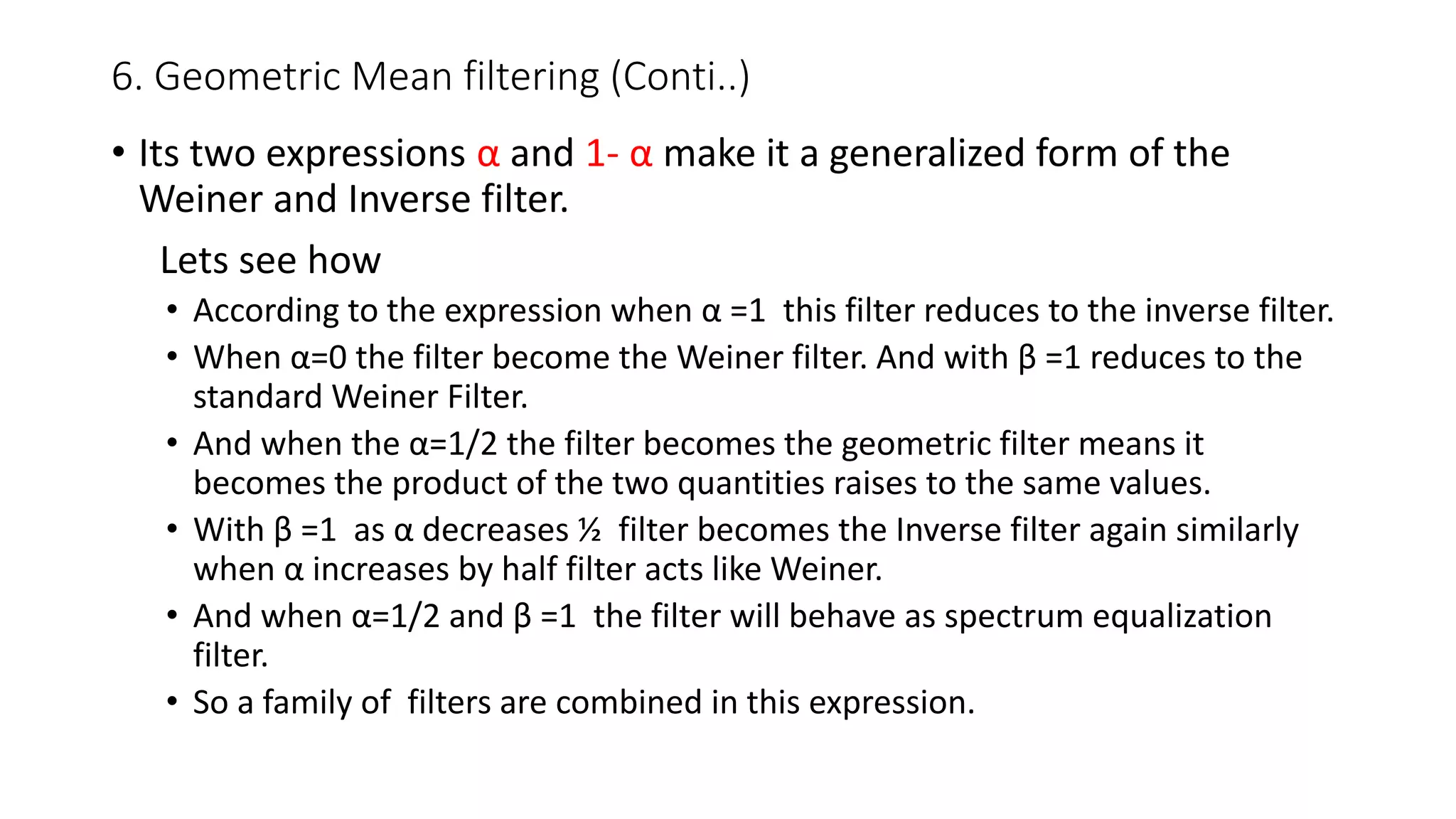
43. 6. Geometric Mean filtering (Conti..)
• Its two expressions α and 1- α make it a generalized form of the
Weiner and Inverse filter.
Lets see how
• According to the expression when α =1 this filter reduces to the inverse filter.
• When α=0 the filter become the Weiner filter. And with β =1 reduces to the
standard Weiner Filter.
• And when the α=1/2 the filter becomes the geometric filter means it
becomes the product of the two quantities raises to the same values.
• With β =1 as α decreases ½ filter becomes the Inverse filter again similarly
when α increases by half filter acts like Weiner.
• And when α=1/2 and β =1 the filter will behave as spectrum equalization
filter.
• So a family of filters are combined in this expression.

44. 6. Geometric Mean filtering (Conti..)
• Example:

45. Implemented Code :
original_image =imread(‘H:moon.jpg');
figure;
imshow(original_image);
title('original image');
[rows,coloumns]=size(original_image);
mu=0;
sigma=sqrt(0.01);
Gauss_noise=mu+sigma*randn(rows,coloumns);
image=im2double(original_image);
noisy_image=zeros(size(image));
for i=1:rows
for j=1:coloumns
noisy_image(i,j)=image(i,j)+Gauss_noise(i,j);
end
end
figure;
imshow(noisy_image,[]);
title('Gaussian Noise corrupted image');
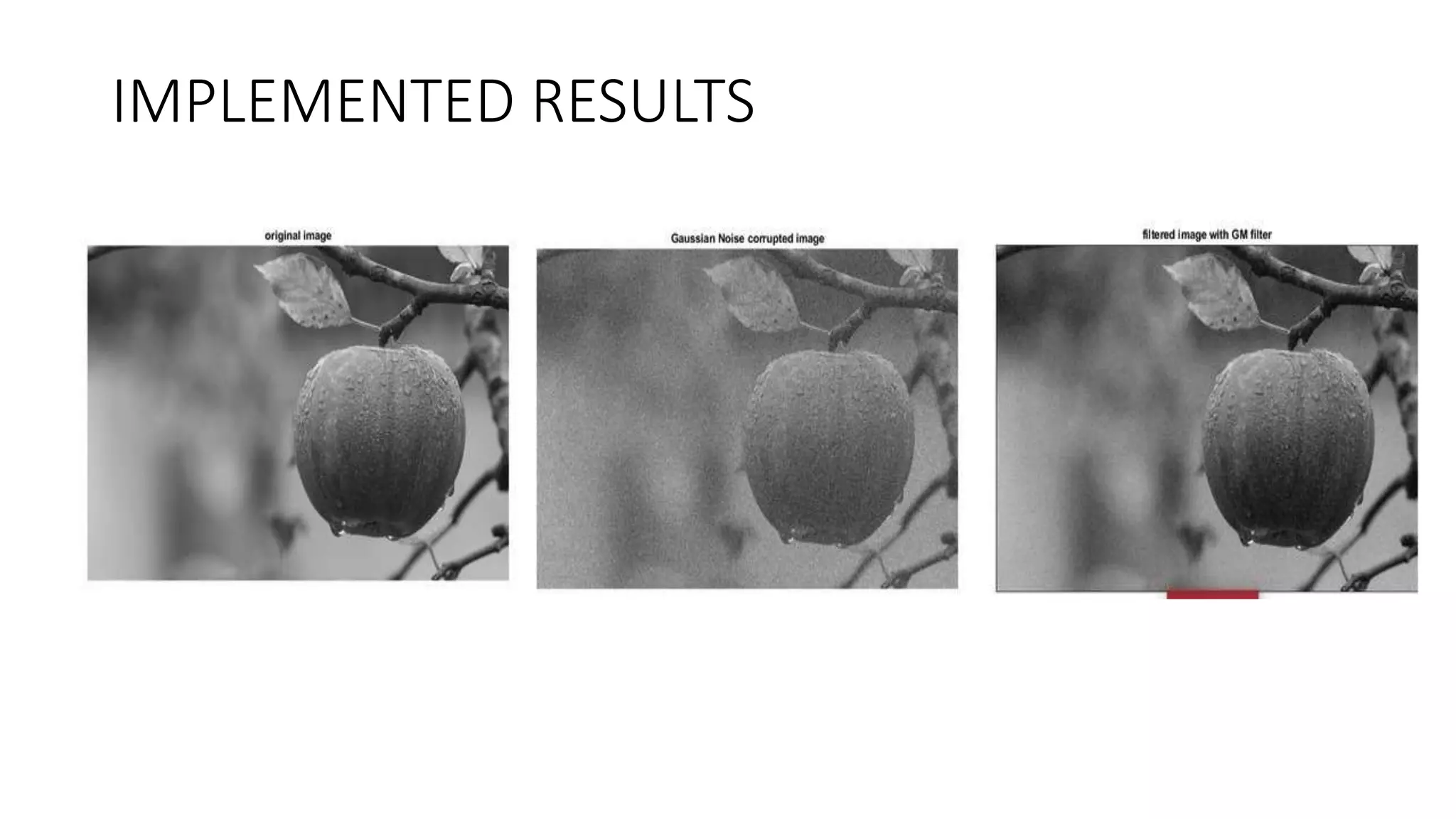
6. Geometric Mean filtering (Hands-on Practices-Hour)
Implemented Code:
m=3;
n=3;
padded_image=zeros((m-1)+size(noisy_image,1),(n-
1)+size(noisy_image,2));
padded_image((m-1)/2+1:(m-1)/2+size(noisy_image,1),(n-
1)/2+1:(n-1)/2+size(noisy_image,2))=noisy_image;
filtered_image=zeros(size(noisy_image));
for i=(m-1)/2+1:(m-1)/2+size(noisy_image,1)
for j=(n-1)/2+1:(n-1)/2+size(noisy_image,2)
S_xy =padded_image(i-(m-1)/2:i+(m-1)/2,j-(m-1)/2:j+(m-
1)/2);
filtered_image(i,j)=(prod(S_xy(:)))^(1/(m*n));
end
end
figure;
imshow(filtered_image,[]);
title('filtered image with GM filter');

46. IMPLEMENTED RESULTS

47. Thank You