Module 3 Computer Vision Image restoration and segmentation
1.
COMPUTER VISION (Module-3)
Dr.Ramesh Wadawadagi
Associate Professor
Department of CSE
SVIT, Bengaluru-560064
ramesh.sw@saividya.ac.in
Image Restoration and Reconstruction
2.
Image Restoration andReconstruction
● The principal goal of restoration techniques is to
improve an image in some predefined sense.
● Restoration attempts to recover an image that has been
degraded by using a priori knowledge of the
degradation phenomenon.
● Restoration techniques are oriented toward modeling
the degradation and applying the inverse process in
order to recover the original image.
● In this chapter, we consider linear, space invariant
restoration models that are applicable in a variety of
restoration situations.
3.
A model ofImage Degradation/Restoration Process
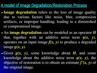
● Image degradation refers to the loss of image quality
due to various factors like noise, blur, compression
artifacts, or improper handling, leading to a diminished
or compromised image.
● An image degradation can be modeled as an operator H
that, together with an additive noise term η(x, y),
operates on an input image f(x, y) to produce a degraded
image g(x, y).
● Given g(x, y), some knowledge about H, and some
knowledge about the additive noise term η(x, y), the
objective of restoration is to obtain an estimate fˆ(x, y) of
the original image.
4.
A model ofImage Degradation/Restoration Process
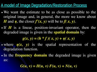
● We want the estimate to be as close as possible to the
original image and, in general, the more we know about
H and η, the closer fˆ(x, y) will be to f( x, y).
● If H is a linear, position-invariant operator, then the
degraded image is given in the spatial domain by:
g(x, y) = (h * f )( x, y) + η( x, y)
● where η(x, y) is the spatial representation of the
degradation function.
● In the frequency domain the degraded image is given
as:
G(u, v) = H(u, v) F(u, v) + N(u, v)
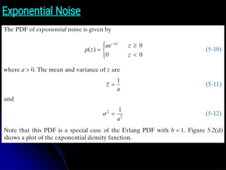
Noise models: Importantnoise probability density functions
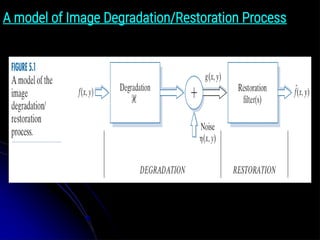
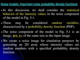
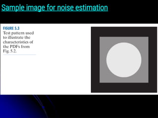
● In this discussion, we shall consider the statistical
behavior of the intensity values in the noise component
of the model in Fig. 5.1.
● These may be considered random variables,
characterized by a probability density function (PDF).
● The noise component of the model in Fig. 5.1 is an
image, η(x, y), of the same size as the input image.
● We create a noise image for simulation purposes by
generating an 2D array whose intensity values are
random numbers with a specified probability density
function.
7.
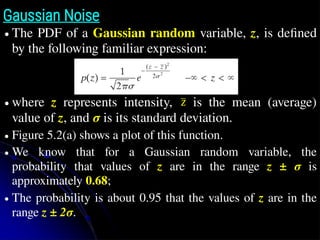
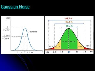
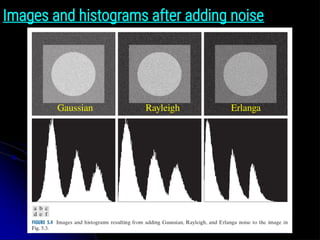
Gaussian Noise
● ThePDF of a Gaussian random variable, z, is defined
by the following familiar expression:
● where z represents intensity, is the mean (average)
value of z, and σ is its standard deviation.
● Figure 5.2(a) shows a plot of this function.
● We know that for a Gaussian random variable, the
probability that values of z are in the range z ± σ is
approximately 0.68;
● The probability is about 0.95 that the values of z are in the
range z ± 2σ.
z̄
z̄
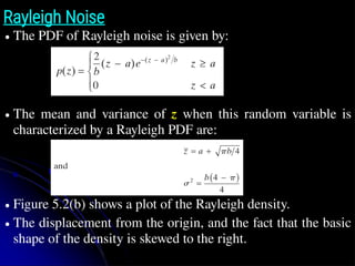
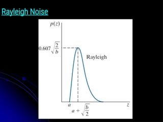
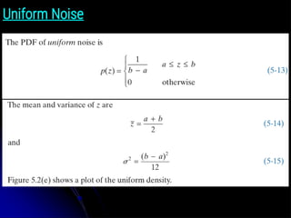
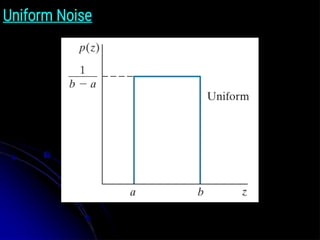
Rayleigh Noise
● ThePDF of Rayleigh noise is given by:
● The mean and variance of z when this random variable is
characterized by a Rayleigh PDF are:
● Figure 5.2(b) shows a plot of the Rayleigh density.
● The displacement from the origin, and the fact that the basic
shape of the density is skewed to the right.
z̄
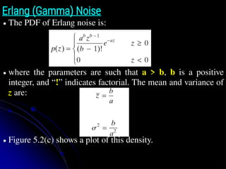
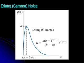
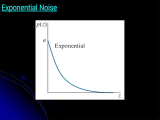
Erlang (Gamma) Noise
●The PDF of Erlang noise is:
● where the parameters are such that a > b, b is a positive
integer, and “!” indicates factorial. The mean and variance of
z are:
● Figure 5.2(c) shows a plot of this density.
z̄
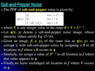
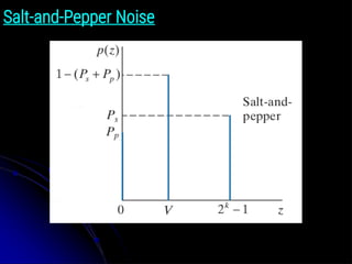
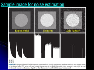
Salt-and-Pepper Noise
● ThePDF of salt-and-pepper noise is given by:
● where V is any integer value in the range 0 < V < 2 k − 1
.
● Let η(x, y) denote a salt-and-pepper noise image, whose
intensity values satisfy Eq. (5-16).
● Given an image, f( x, y), of the same size as η(x, y), we
corrupt it with salt-and-pepper noise by assigning a 0 to all
locations in f where a 0 occurs in η.
● Similarly, we assign a value of 2k − 1
to all location in f where
that value appears in η.
● Finally,we leave unchanged all location in f where V occurs
in η.
z̄
Restoration using spatialfiltering
MEAN FILTERS
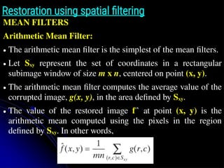
Arithmetic Mean Filter:
● The arithmetic mean filter is the simplest of the mean filters.
● Let Sxy represent the set of coordinates in a rectangular
subimage window of size m x n, centered on point (x, y).
● The arithmetic mean filter computes the average value of the
corrupted image, g(x, y), in the area defined by Sxy.
● The value of the restored image f at point
̂ (x, y) is the
arithmetic mean computed using the pixels in the region
defined by Sxy. In other words,
z̄
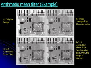
Arithmetic mean filter(Example)
z̄
a) Original
Image
b) Image
corrupted by
Gaussian noise
c) 3x3
Arithmetic
Mean Filter
d) 3x3
Geometric
Mean Filter
(less blurring
than AMF, the
image is
sharper)
25.
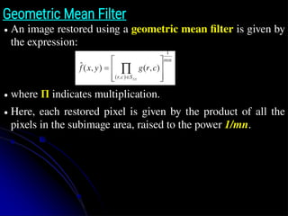
Geometric Mean Filter
●An image restored using a geometric mean filter is given by
the expression:
● where Π indicates multiplication.
● Here, each restored pixel is given by the product of all the
pixels in the subimage area, raised to the power 1/mn.
z̄
∏ g
∏ g(r ,c)
26.
z̄
∏ g(r ,c)
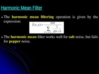
HarmonicMean Filter
● The harmonic mean filtering operation is given by the
expression:
● The harmonic mean filter works well for salt noise, but fails
for pepper noise.
27.
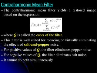
Contraharmonic Mean Filter
●The contraharmonic mean filter yields a restored image
based on the expression:
● where Q is called the order of the filter.
● This filter is well suited for reducing or virtually eliminating
the effects of salt-and-pepper noise.
● For positive values of Q, the filter eliminates pepper noise.
● For negetive values of Q, the filter eliminates salt noise.
● It cannot do both simultaneously.
28.
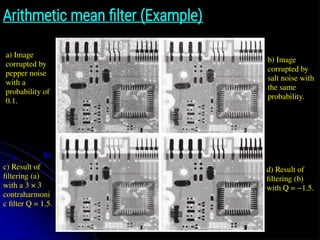
Arithmetic mean filter(Example)
z̄
a) Image
corrupted by
pepper noise
with a
probability of
0.1.
b) Image
corrupted by
salt noise with
the same
probability.
c) Result of
filtering (a)
with a 3 × 3
contraharmoni
c filter Q = 1.5.
d) Result of
filtering (b)
with Q = −1.5.
29.
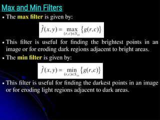
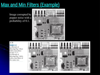
Max and MinFilters
● The max filter is given by:
● This filter is useful for finding the brightest points in an
image or for eroding dark regions adjacent to bright areas.
● The min filter is given by:
● This filter is useful for finding the darkest points in an image
or for eroding light regions adjacent to dark areas.
30.
Max and MinFilters (Example)
Image corrupted by
pepper noise with a
probability of 0.1.
31.
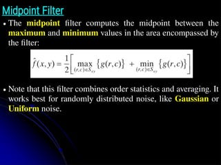
Midpoint Filter
● Themidpoint filter computes the midpoint between the
maximum and minimum values in the area encompassed by
the filter:
● Note that this filter combines order statistics and averaging. It
works best for randomly distributed noise, like Gaussian or
Uniform noise.
32.
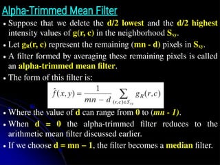
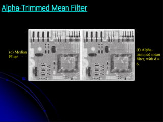
Alpha-Trimmed Mean Filter
●Suppose that we delete the d/2 lowest and the d/2 highest
intensity values of g(r, c) in the neighborhood Sxy.
● Let gR(r, c) represent the remaining (mn - d) pixels in Sxy.
● A filter formed by averaging these remaining pixels is called
an alpha-trimmed mean filter.
● The form of this filter is:
● Where the value of d can range from 0 to (mn - 1).
● When d = 0 the alpha-trimmed filter reduces to the
arithmetic mean filter discussed earlier.
● If we choose d = mn − 1, the filter becomes a median filter.
33.
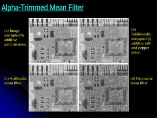
Alpha-Trimmed Mean Filter
(a)Image
corrupted by
additive
uniform noise.
(b)
Additionally
corrupted by
additive salt-
and-pepper
noise.
(c) Arithmetic
mean filter
(d) Geometric
mean filter
ADAPTIVE FILTERS
● Thefilters discussed thus far are applied to an image without
regard for how image characteristics vary from one point to
another.
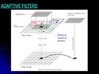
● In this section, we take a look at two adaptive filters whose
behavior changes based on statistical characteristics of the
image inside the filter region defined by the mxn rectangular
neighborhood Sxy.
● Adaptive filters are capable of performing superior to that of
the filters discussed thus far.
● However, they are expensive in terms of computational time.
1. Adaptive, LocalNoise Reduction Filter
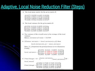
● The simplest statistical measures of a random variable are its
mean and variance.
● These are reasonable parameters on which to base an
adaptive filter because they are quantities closely related to
the appearance of an image.
● The mean gives a measure of average intensity in the image
region.
● Variance gives a measure of image contrast in that region.
38.
Adaptive, Local NoiseReduction Filter
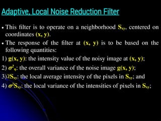
● This filter is to operate on a neighborhood Sxy, centered on
coordinates (x, y).
● The response of the filter at (x, y) is to be based on the
following quantities:
1) g(x, y): the intensity value of the noisy image at (x, y);
2) σ2
η: the overall variance of the noise image g(x, y);
3) Sxy: the local average intensity of the pixels in Sxy; and
4) σ2
Sxy: the local variance of the intensities of pixels in Sxy;
z̄
39.
Adaptive, Local NoiseReduction Filter
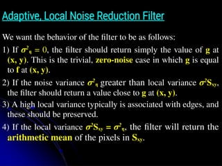
We want the behavior of the filter to be as follows:
1) If σ2
η = 0, the filter should return simply the value of g at
(x, y). This is the trivial, zero-noise case in which g is equal
to f at (x, y).
2) If the noise variance σ2
η greater than local variance σ2
Sxy,
the filter should return a value close to g at (x, y).
3) A high local variance typically is associated with edges, and
these should be preserved.
4) If the local variance σ2
Sxy = σ2
η, the filter will return the
arithmetic mean of the pixels in Sxy.
40.
Adaptive, Local NoiseReduction Filter
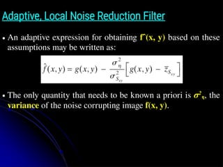
● An adaptive expression for obtaining fˆ(x, y) based on these
assumptions may be written as:
● The only quantity that needs to be known a priori is σ2
η, the
variance of the noise corrupting image f(x, y).
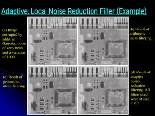
Adaptive, Local NoiseReduction Filter (Example)
(a) Image
corrupted by
additive
Gaussian noise
of zero mean
and a variance
of 1000.
(b) Result of
arithmetic
mean filtering.
(c) Result of
geometric
mean filtering.
(d) Result of
adaptive
noise-
reduction
filtering. All
filters used
were of size
7 × 7.
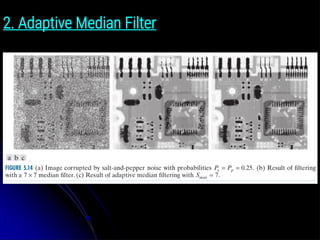
44.
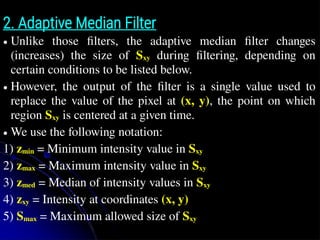
2. Adaptive MedianFilter
● Unlike those filters, the adaptive median filter changes
(increases) the size of Sxy during filtering, depending on
certain conditions to be listed below.
● However, the output of the filter is a single value used to
replace the value of the pixel at (x, y), the point on which
region Sxy is centered at a given time.
● We use the following notation:
1) zmin = Minimum intensity value in Sxy
2) zmax = Maximum intensity value in Sxy
3) zmed = Median of intensity values in Sxy
4) zxy = Intensity at coordinates (x, y)
5) Smax = Maximum allowed size of Sxy
45.
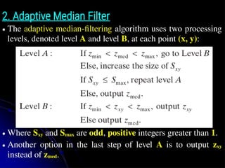
2. Adaptive MedianFilter
● The adaptive median-filtering algorithm uses two processing
levels, denoted level A and level B, at each point (x, y):
● Where Sxy and Smax are odd, positive integers greater than 1.
● Another option in the last step of level A is to output zxy
instead of zmed.
PERIODIC NOISE REDUCTIONUSING FREQUENCY DOMAIN FILTERING
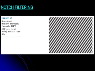
NOTCH FILTERING
● The general form of a notch filter transfer function is:
● Where Hk(u, v) and H-k(u, v) are highpass filter transfer
functions whose centers are at (uk , vk) and (−uk, −vk),
respectively.
● These centers are specified with respect to the center of the
frequency rectangle, [floor(M/2), floor(N/2)], where M and
N are the number of rows and columns in the input image.
48.
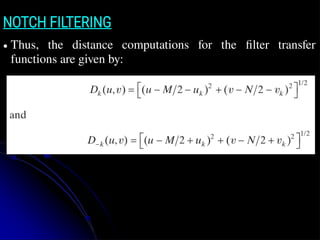
NOTCH FILTERING
● Thus,the distance computations for the filter transfer
functions are given by:
COMPUTER VISION (Module-3)
Dr.Ramesh Wadawadagi
Associate Professor
Department of CSE
SVIT, Bengaluru-560064
ramesh.sw@saividya.ac.in
Image Segmentation
52.
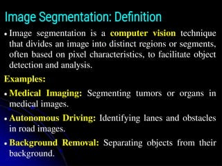
Image Segmentation: Definition
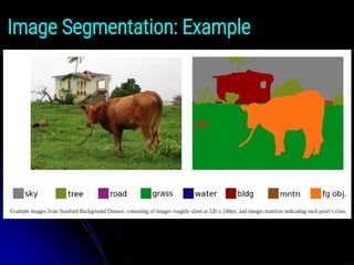
●Image segmentation is a computer vision technique
that divides an image into distinct regions or segments,
often based on pixel characteristics, to facilitate object
detection and analysis.
Examples:
● Medical Imaging: Segmenting tumors or organs in
medical images.
● Autonomous Driving: Identifying lanes and obstacles
in road images.
● Background Removal: Separating objects from their
background.
53.
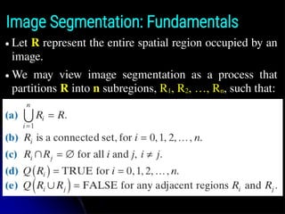
Image Segmentation: Fundamentals
●Let R represent the entire spatial region occupied by an
image.
● We may view image segmentation as a process that
partitions R into n subregions, R1, R2, …, Rn, such that:
54.
Image Segmentation: Fundamentals
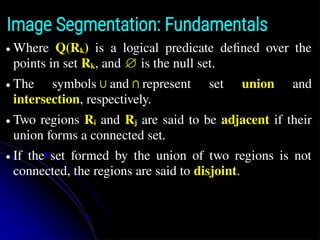
●Where Q(Rk) is a logical predicate defined over the
points in set Rk, and ∅ is the null set.
● The symbols∪and∩represent set union and
intersection, respectively.
● Two regions Ri and Rj are said to be adjacent if their
union forms a connected set.
● If the set formed by the union of two regions is not
connected, the regions are said to disjoint.
Image Segmentation: Fundamentals
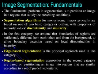
●The fundamental problem in segmentation is to partition an image
into regions that satisfy the preceding conditions.
● Segmentation algorithms for monochrome images generally are
based on one of two basic categories dealing with properties of
intensity values: discontinuity and similarity.
● In the first category, we assume that boundaries of regions are
sufficiently different from each other, and from the background, to
allow boundary detection based on local discontinuities in
intensity.
● Edge-based segmentation is the principal approach used in this
category.
● Region-based segmentation approaches in the second category
are based on partitioning an image into regions that are similar
according to a set of predefined criteria.
57.
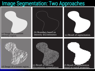
Image Segmentation: TwoApproaches
(a) Image of a constant
intensity region.
(b) Boundary based on
intensity discontinuities (c) Result of segmentation.
(d) Image of a texture region.
(e) Result of intensity
discontinuity computations
(f) Result of segmentation
based on region properties.
58.
POINT, LINE, ANDEDGE DETECTION
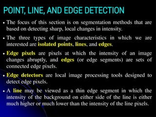
● The focus of this section is on segmentation methods that are
based on detecting sharp, local changes in intensity.
● The three types of image characteristics in which we are
interested are isolated points, lines, and edges.
● Edge pixels are pixels at which the intensity of an image
changes abruptly, and edges (or edge segments) are sets of
connected edge pixels.
● Edge detectors are local image processing tools designed to
detect edge pixels.
● A line may be viewed as a thin edge segment in which the
intensity of the background on either side of the line is either
much higher or much lower than the intensity of the line pixels.
59.
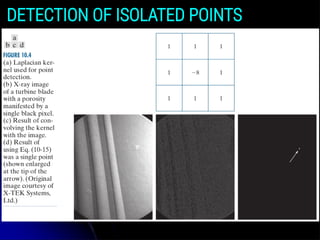
DETECTION OF ISOLATEDPOINTS
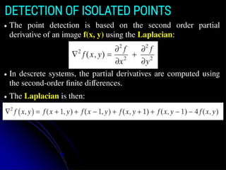
● The point detection is based on the second order partial
derivative of an image f(x, y) using the Laplacian:
● In descrete systems, the partial derivatives are computed using
the second-order finite differences.
● The Laplacian is then:
60.
DETECTION OF ISOLATEDPOINTS
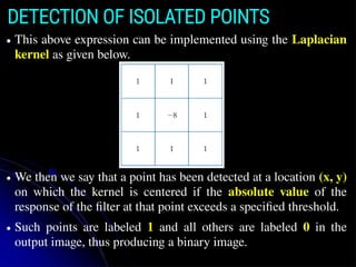
● This above expression can be implemented using the Laplacian
kernel as given below.
● We then we say that a point has been detected at a location (x, y)
on which the kernel is centered if the absolute value of the
response of the filter at that point exceeds a specified threshold.
● Such points are labeled 1 and all others are labeled 0 in the
output image, thus producing a binary image.
61.
DETECTION OF ISOLATEDPOINTS
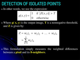
● In other words, we use the expression:
● Where g( x, y) is the output image, T is a nonnegative threshold,
and Z is given by:
● This formulation simply measures the weighted differences
between a pixel and its 8-neighbors.
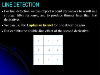
LINE DETECTION
● Forline detection we can expect second derivatives to result in a
stronger filter response, and to produce thinner lines than first
derivatives.
● We can use the Laplacian kernel for line detection also.
● But exhibits the double-line effect of the second derivative.
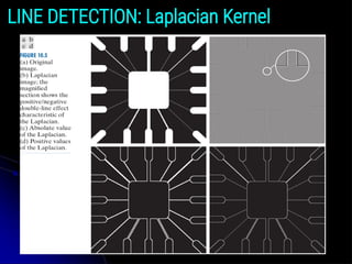
LINE DETECTION: LaplacianKernel
● Because the Laplacian image contains negative values, scaling
is necessary for display.
● As the magnified section shows, mid gray represents zero,
darker shades of gray represent negative values, and lighter
shades are positive.
● The double-line effect is clearly visible in the magnified region.
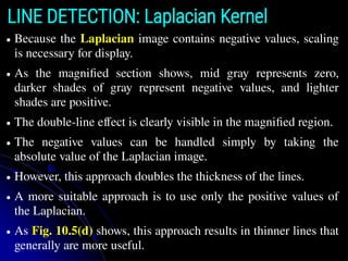
● The negative values can be handled simply by taking the
absolute value of the Laplacian image.
● However, this approach doubles the thickness of the lines.
● A more suitable approach is to use only the positive values of
the Laplacian.
● As Fig. 10.5(d) shows, this approach results in thinner lines that
generally are more useful.
66.
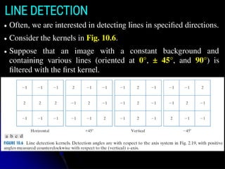
LINE DETECTION
● Often,we are interested in detecting lines in specified directions.
● Consider the kernels in Fig. 10.6.
● Suppose that an image with a constant background and
containing various lines (oriented at 0°, ± 45°, and 90°) is
filtered with the first kernel.
67.
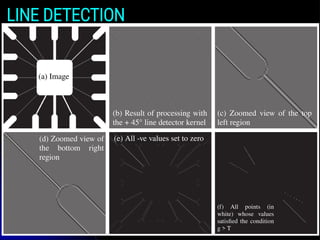
LINE DETECTION
(a) Image
(b)Result of processing with
the + 45° line detector kernel
(c) Zoomed view of the top
left region
(d) Zoomed view of
the bottom right
region
(e) All -ve values set to zero
(f) All points (in
white) whose values
satisfied the condition
g > T
68.
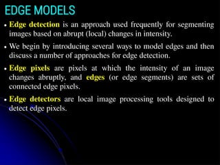
EDGE MODELS
● Edgedetection is an approach used frequently for segmenting
images based on abrupt (local) changes in intensity.
● We begin by introducing several ways to model edges and then
discuss a number of approaches for edge detection.
● Edge pixels are pixels at which the intensity of an image
changes abruptly, and edges (or edge segments) are sets of
connected edge pixels.
● Edge detectors are local image processing tools designed to
detect edge pixels.
69.
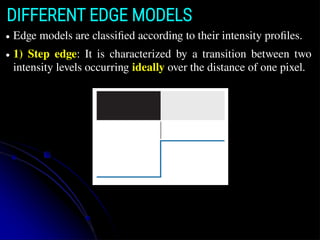
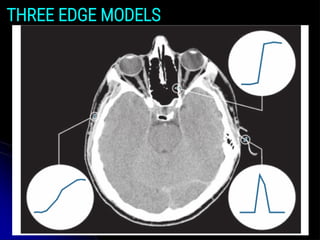
DIFFERENT EDGE MODELS
●Edge models are classified according to their intensity profiles.
● 1) Step edge: It is characterized by a transition between two
intensity levels occurring ideally over the distance of one pixel.
70.
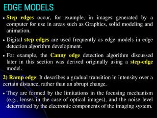
EDGE MODELS
● Stepedges occur, for example, in images generated by a
computer for use in areas such as Graphics, solid modeling and
animation.
● Digital step edges are used frequently as edge models in edge
detection algorithm development.
● For example, the Canny edge detection algorithm discussed
later in this section was derived originally using a step-edge
model.
2) Ramp edge: It describes a gradual transition in intensity over a
certain distance, rather than an abrupt change.
● They are formed by the limitations in the focusing mechanism
(e.g., lenses in the case of optical images), and the noise level
determined by the electronic components of the imaging system.
71.
EDGE MODELS
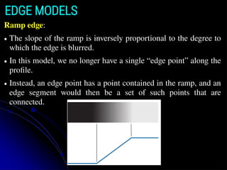
Ramp edge:
●The slope of the ramp is inversely proportional to the degree to
which the edge is blurred.
● In this model, we no longer have a single “edge point” along the
profile.
● Instead, an edge point has a point contained in the ramp, and an
edge segment would then be a set of such points that are
connected.
72.
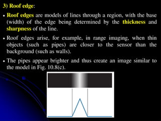
3) Roof edge:
●Roof edges are models of lines through a region, with the base
(width) of the edge being determined by the thickness and
sharpness of the line.
● Roof edges arise, for example, in range imaging, when thin
objects (such as pipes) are closer to the sensor than the
background (such as walls).
● The pipes appear brighter and thus create an image similar to
the model in Fig. 10.8(c).
● The magnitudeof the first partial derivative of f(x, y) can be
used to detect the presence of an edge at a point in an image.
● Similarly, the sign of the second partial derivative can be used to
determine whether an edge pixel lies on the dark or light side of
an edge.
● Two additional properties of the second derivative around an
edge are:
(1) It produces two values for every edge in an image; and
(2) Its zero crossings can be used for locating the centers of thick
edges, as we will show later in this section.
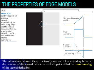
THE PROPERTIES OF EDGE MODELS
75.
THE PROPERTIES OFEDGE MODELS
The intersection between the zero intensity axis and a line extending between the extrema of
the second derivative marks a point called the zero crossing of the second derivative.
The intersection between the zero intensity axis and a line extending between
the extrema of the second derivative marks a point called the zero crossing
of the second derivative.
76.
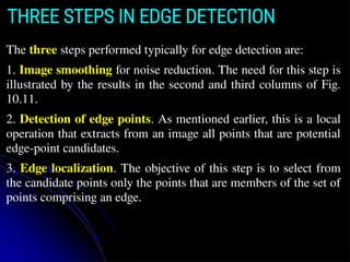
The three stepsperformed typically for edge detection are:
1. Image smoothing for noise reduction. The need for this step is
illustrated by the results in the second and third columns of Fig.
10.11.
2. Detection of edge points. As mentioned earlier, this is a local
operation that extracts from an image all points that are potential
edge-point candidates.
3. Edge localization. The objective of this step is to select from
the candidate points only the points that are members of the set of
points comprising an edge.
THREE STEPS IN EDGE DETECTION
77.
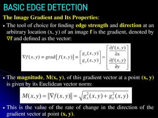
The Image Gradientand Its Properties:
● The tool of choice for finding edge strength and direction at an
arbitrary location (x, y) of an image f is the gradient, denoted by
∇f and defined as the vector:
● The magnitude, M(x, y), of this gradient vector at a point (x, y)
is given by its Euclidean vector norm:
● This is the value of the rate of change in the direction of the
gradient vector at point (x, y).
BASIC EDGE DETECTION
78.
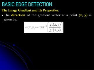
The Image Gradientand Its Properties:
● The direction of the gradient vector at a point (x, y) is
given by:
BASIC EDGE DETECTION
79.
BASIC EDGE DETECTION
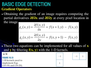
GradientOperators
● Obtaining the gradient of an image requires computing the
partial derivatives ∂f/∂x and ∂f/∂y at every pixel location in
the image.
● These two equations can be implemented for all values of x
and y by filtering f(x, y) with the 1-D kernels.
80.
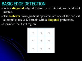
BASIC EDGE DETECTION
●When diagonal edge direction is of interest, we need 2-D
kernels.
● The Roberts cross-gradient operators are one of the earliest
attempts to use 2-D kernels with a diagonal preference.
● Consider the 3 × 3 region.
81.
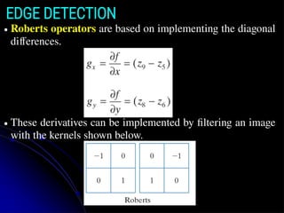
EDGE DETECTION
● Robertsoperators are based on implementing the diagonal
differences.
● These derivatives can be implemented by filtering an image
with the kernels shown below.
82.
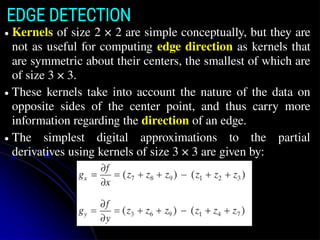
EDGE DETECTION
● Kernelsof size 2 × 2 are simple conceptually, but they are
not as useful for computing edge direction as kernels that
are symmetric about their centers, the smallest of which are
of size 3 × 3.
● These kernels take into account the nature of the data on
opposite sides of the center point, and thus carry more
information regarding the direction of an edge.
● The simplest digital approximations to the partial
derivatives using kernels of size 3 × 3 are given by:
83.
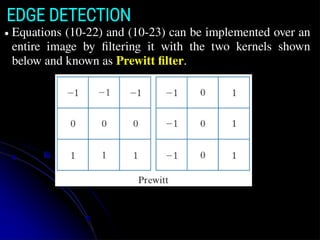
EDGE DETECTION
● Equations(10-22) and (10-23) can be implemented over an
entire image by filtering it with the two kernels shown
below and known as Prewitt filter.
84.
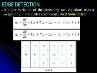
EDGE DETECTION
● Aslight variation of the preceding two equations uses a
weight of 2 in the center coefficient called Sobel filter:
85.
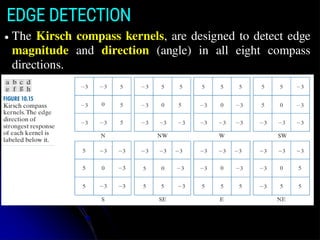
EDGE DETECTION
● TheKirsch compass kernels, are designed to detect edge
magnitude and direction (angle) in all eight compass
directions.
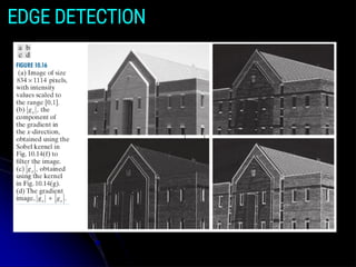
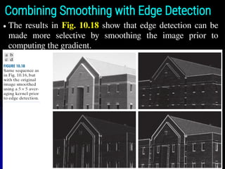
Combining Smoothing withEdge Detection
● The results in Fig. 10.18 show that edge detection can be
made more selective by smoothing the image prior to
computing the gradient.
88.
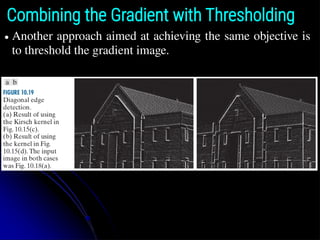
Combining the Gradientwith Thresholding
● Another approach aimed at achieving the same objective is
to threshold the gradient image.
89.
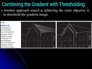
Combining the Gradientwith Thresholding
● Another approach aimed at achieving the same objective is
to threshold the gradient image.
90.
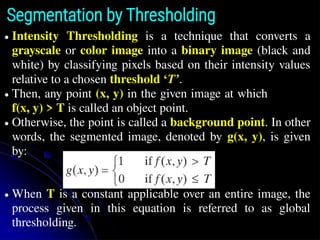
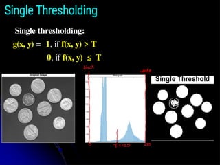
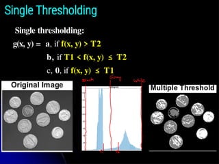
Segmentation by Thresholding
●Intensity Thresholding is a technique that converts a
grayscale or color image into a binary image (black and
white) by classifying pixels based on their intensity values
relative to a chosen threshold ‘T’.
● Then, any point (x, y) in the given image at which
f(x, y) > T is called an object point.
● Otherwise, the point is called a background point. In other
words, the segmented image, denoted by g(x, y), is given
by:
● When T is a constant applicable over an entire image, the
process given in this equation is referred to as global
thresholding.
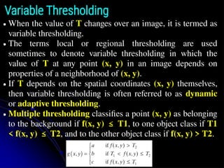
Variable Thresholding
● Whenthe value of T changes over an image, it is termed as
variable thresholding.
● The terms local or regional thresholding are used
sometimes to denote variable thresholding in which the
value of T at any point (x, y) in an image depends on
properties of a neighborhood of (x, y).
● If T depends on the spatial coordinates (x, y) themselves,
then variable thresholding is often referred to as dynamic
or adaptive thresholding.
● Multiple thresholding classifies a point (x, y) as belonging
to the background if f(x, y) ≤ T1, to one object class if T1
< f(x, y) ≤ T2, and to the other object class if f(x, y) > T2.
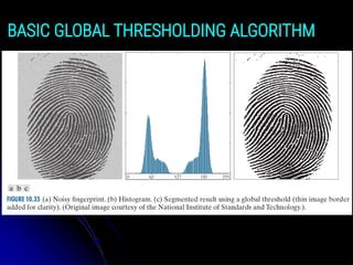
BASIC GLOBAL THRESHOLDING
●When the intensity distributions of objects and
background pixels are sufficiently distinct, it is
possible to use a single (global) threshold
applicable over the entire image.
● In most applications, there is usually enough
variability between the images.
● Hence, an algorithm capable of estimating the
threshold value for each image is required.
● The following iterative algorithm can be used for
this purpose:
SEGMENTATION BY REGIONGROWING
● Region growing is a procedure that groups pixels or
subregions into larger regions based on some
predefined criteria.
● The basic approach is to start with a set of “seed
points”, and from these grow regions by appending to
each seed those neighboring pixels that have predefined
properties similar to the seed.
● Selecting a set of one or more starting points can often
be based on the nature of the problem.
● When a priori information is not available, the
procedure is to compute at every pixel the same set of
properties that ultimately will be used to assign pixels
to regions during the growing process.
98.
SEGMENTATION BY REGIONGROWING
● If the result of these computations forms clusters of
values, the pixels whose properties place them near the
centroid of these clusters can be used as seeds.
● The selection of similarity criteria depends not only on
the problem under consideration, but also on the type
of image data available.
● For example, the analysis of land-use satellite imagery
depends heavily on the use of color.
● This problem would be significantly more difficult, or
even impossible, to solve without the inherent
information available in color images.
99.
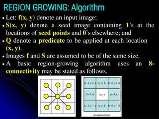
REGION GROWING: Algorithm
●Let: f(x, y) denote an input image;
● S(x, y) denote a seed image containing 1’s at the
locations of seed points and 0’s elsewhere; and
● Q denote a predicate to be applied at each location
(x, y).
● Images f and S are assumed to be of the same size.
● A basic region-growing algorithm uses an 8-
connectivity may be stated as follows.
100.
REGION GROWING: Algorithm
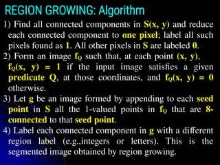
1)Find all connected components in S(x, y) and reduce
each connected component to one pixel; label all such
pixels found as 1. All other pixels in S are labeled 0.
2) Form an image fQ such that, at each point (x, y),
fQ(x, y) = 1 if the input image satisfies a given
predicate Q, at those coordinates, and fQ(x, y) = 0
otherwise.
3) Let g be an image formed by appending to each seed
point in S all the 1-valued points in fQ that are 8-
connected to that seed point.
4) Label each connected component in g with a different
region label (e.g.,integers or letters). This is the
segmented image obtained by region growing.
101.
EXAMPLE: Segmentation byregion growing
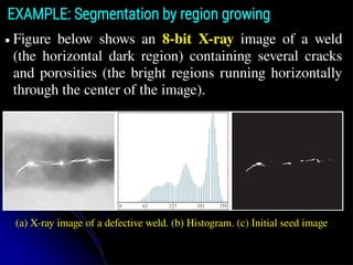
● Figure below shows an 8-bit X-ray image of a weld
(the horizontal dark region) containing several cracks
and porosities (the bright regions running horizontally
through the center of the image).
(a) X-ray image of a defective weld. (b) Histogram. (c) Initial seed image
102.
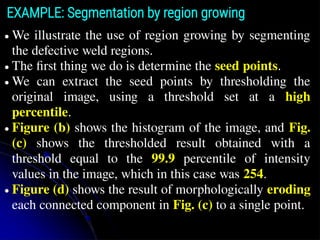
● We illustratethe use of region growing by segmenting
the defective weld regions.
● The first thing we do is determine the seed points.
● We can extract the seed points by thresholding the
original image, using a threshold set at a high
percentile.
● Figure (b) shows the histogram of the image, and Fig.
(c) shows the thresholded result obtained with a
threshold equal to the 99.9 percentile of intensity
values in the image, which in this case was 254.
● Figure (d) shows the result of morphologically eroding
each connected component in Fig. (c) to a single point.
EXAMPLE: Segmentation by region growing
103.
EXAMPLE: Segmentation byregion growing
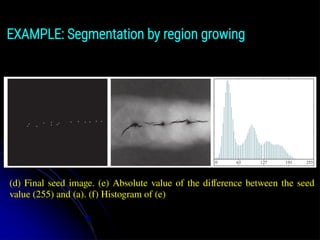
(d) Final seed image. (e) Absolute value of the difference between the seed
value (255) and (a). (f) Histogram of (e)
104.
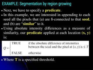
● Next, wehave to specify a predicate.
● In this example, we are interested in appending to each
seed all the pixels that (a) are 8-connected to that seed,
and (b) are “similar” to it.
● Using absolute intensity differences as a measure of
similarity, our predicate applied at each location (x, y)
is:
● Where T is a specified threshold.
EXAMPLE: Segmentation by region growing
105.
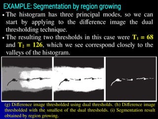
● The histogramhas three principal modes, so we can
start by applying to the difference image the dual
thresholding technique.
● The resulting two thresholds in this case were T1 = 68
and T2 = 126, which we see correspond closely to the
valleys of the histogram.
EXAMPLE: Segmentation by region growing
(g) Difference image thresholded using dual thresholds. (h) Difference image
thresholded with the smallest of the dual thresholds. (i) Segmentation result
obtained by region growing.
106.
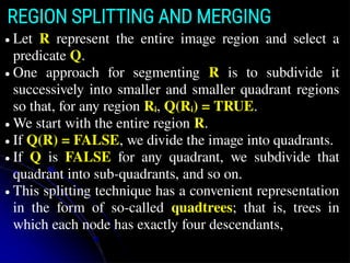
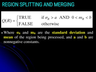
REGION SPLITTING ANDMERGING
● Let R represent the entire image region and select a
predicate Q.
● One approach for segmenting R is to subdivide it
successively into smaller and smaller quadrant regions
so that, for any region Ri, Q(Ri) = TRUE.
● We start with the entire region R.
● If Q(R) = FALSE, we divide the image into quadrants.
● If Q is FALSE for any quadrant, we subdivide that
quadrant into sub-quadrants, and so on.
● This splitting technique has a convenient representation
in the form of so-called quadtrees; that is, trees in
which each node has exactly four descendants,
107.
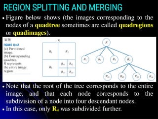
REGION SPLITTING ANDMERGING
● Figure below shows (the images corresponding to the
nodes of a quadtree sometimes are called quadregions
or quadimages).
● Note that the root of the tree corresponds to the entire
image, and that each node corresponds to the
subdivision of a node into four descendant nodes.
● In this case, only R4 was subdivided further.
108.
REGION SPLITTING ANDMERGING
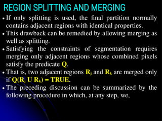
● If only splitting is used, the final partition normally
contains adjacent regions with identical properties.
● This drawback can be remedied by allowing merging as
well as splitting.
● Satisfying the constraints of segmentation requires
merging only adjacent regions whose combined pixels
satisfy the predicate Q.
● That is, two adjacent regions Rj and Rk are merged only
if Q(Rj U Rk) = TRUE.
● The preceding discussion can be summarized by the
following procedure in which, at any step, we,
109.
REGION SPLITTING ANDMERGING
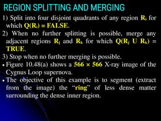
1) Split into four disjoint quadrants of any region Ri for
which Q(Ri) = FALSE.
2) When no further splitting is possible, merge any
adjacent regions Rj and Rk for which Q(Rj U Rk) =
TRUE.
3) Stop when no further merging is possible.
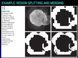
● Figure 10.48(a) shows a 566 × 566 X-ray image of the
Cygnus Loop supernova.
● The objective of this example is to segment (extract
from the image) the “ring” of less dense matter
surrounding the dense inner region.
REGION SPLITTING ANDMERGING
● The region of interest has some obvious characteristics
that should help in its segmentation.
● First, we note that the data in this region has a random
nature, indicating that its standard deviation should be
greater than the standard deviation of the background
(which is near 0) and of the large central region, which
is smooth.
● Similarly, the mean value (average intensity) of a
region containing data from the outer ring should be
greater than the mean of the darker background and
less than the mean of the lighter central region.
● Thus, we should be able to segment the region of
interest using the following predicate:
112.
REGION SPLITTING ANDMERGING
● Where σR and mR are the standard deviation and
mean of the region being processed, and a and b are
nonnegative constants.


![PERIODIC NOISE REDUCTION USING FREQUENCY DOMAIN FILTERING
NOTCH FILTERING
● The general form of a notch filter transfer function is:
● Where Hk(u, v) and H-k(u, v) are highpass filter transfer
functions whose centers are at (uk , vk) and (−uk, −vk),
respectively.
● These centers are specified with respect to the center of the
frequency rectangle, [floor(M/2), floor(N/2)], where M and
N are the number of rows and columns in the input image.](https://image.slidesharecdn.com/module3computervisioncomplete-250417040843-e99a9dee/85/Module-3-Computer-Vision-Image-restoration-and-segmentation-47-320.jpg)