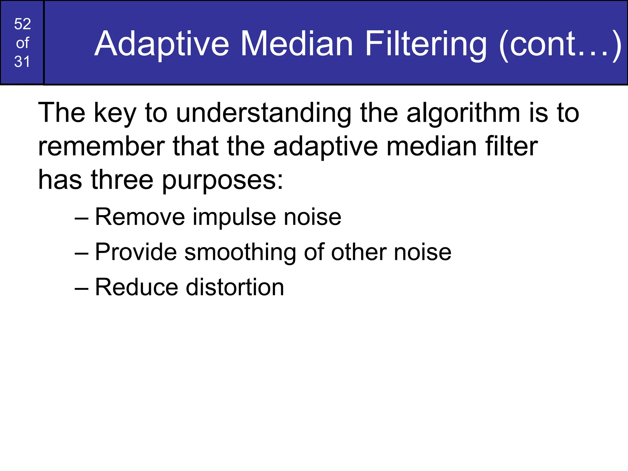
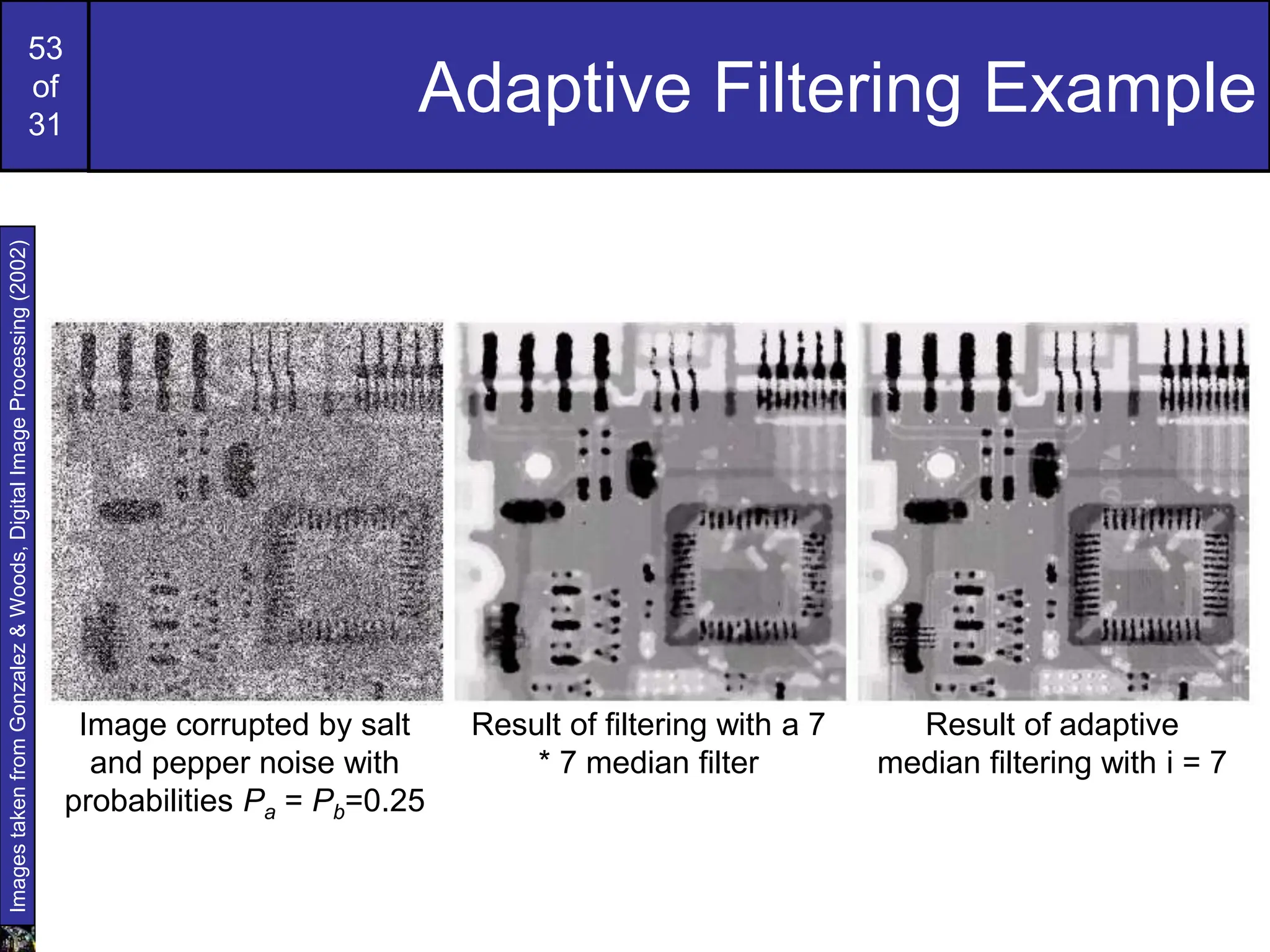
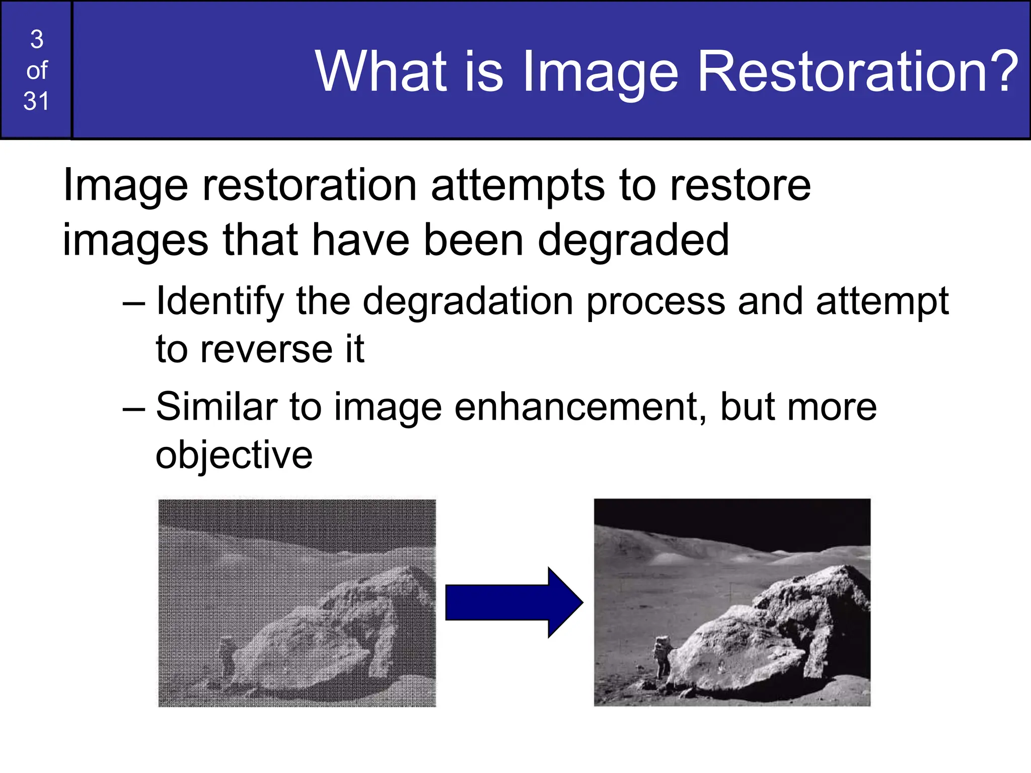
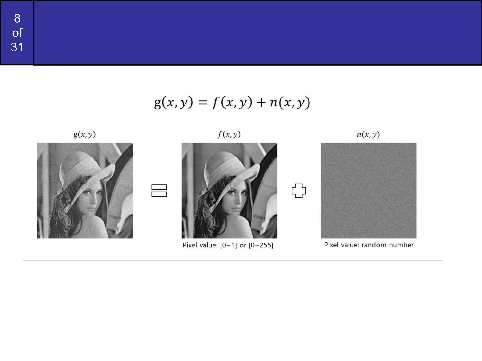
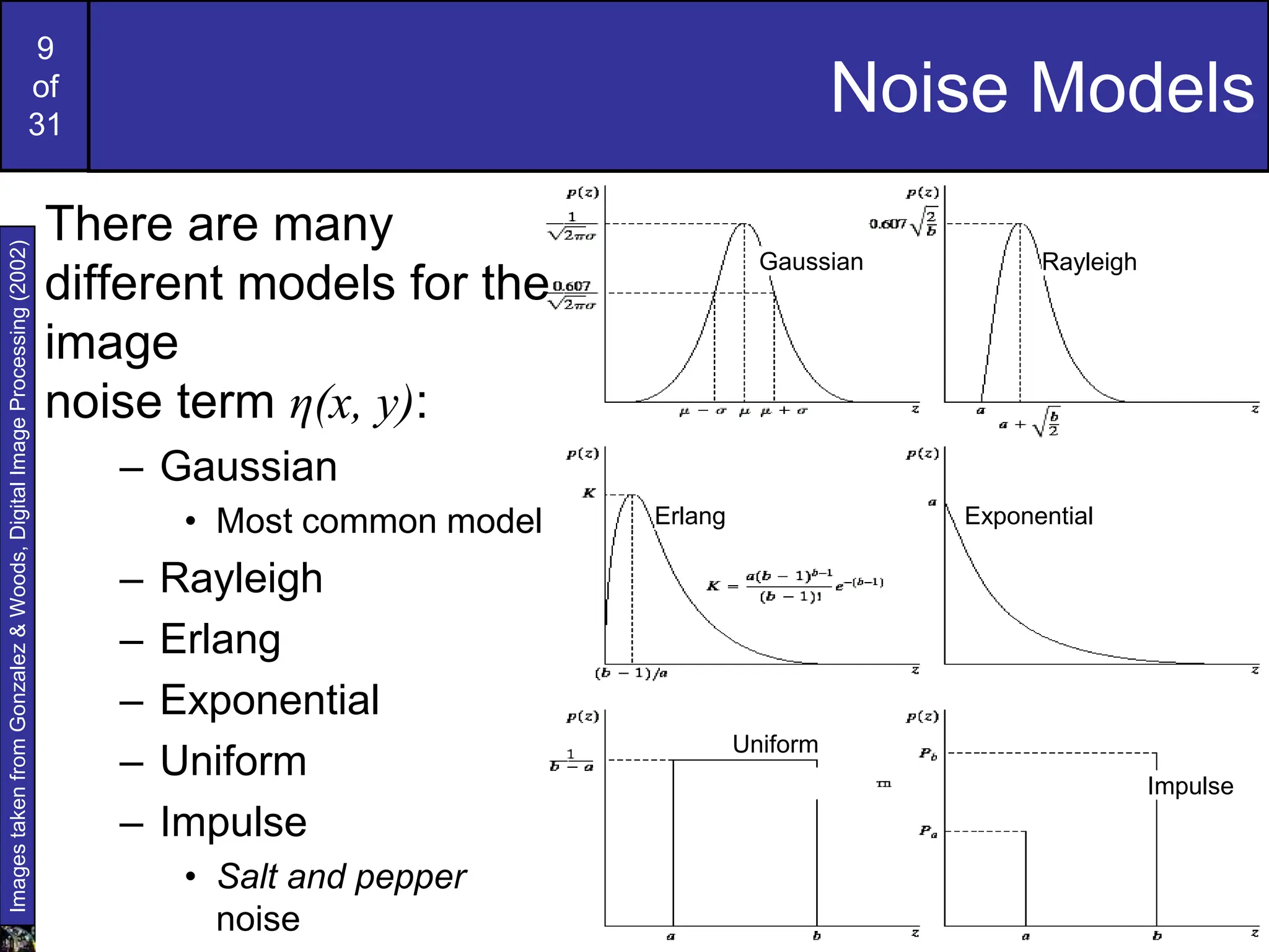
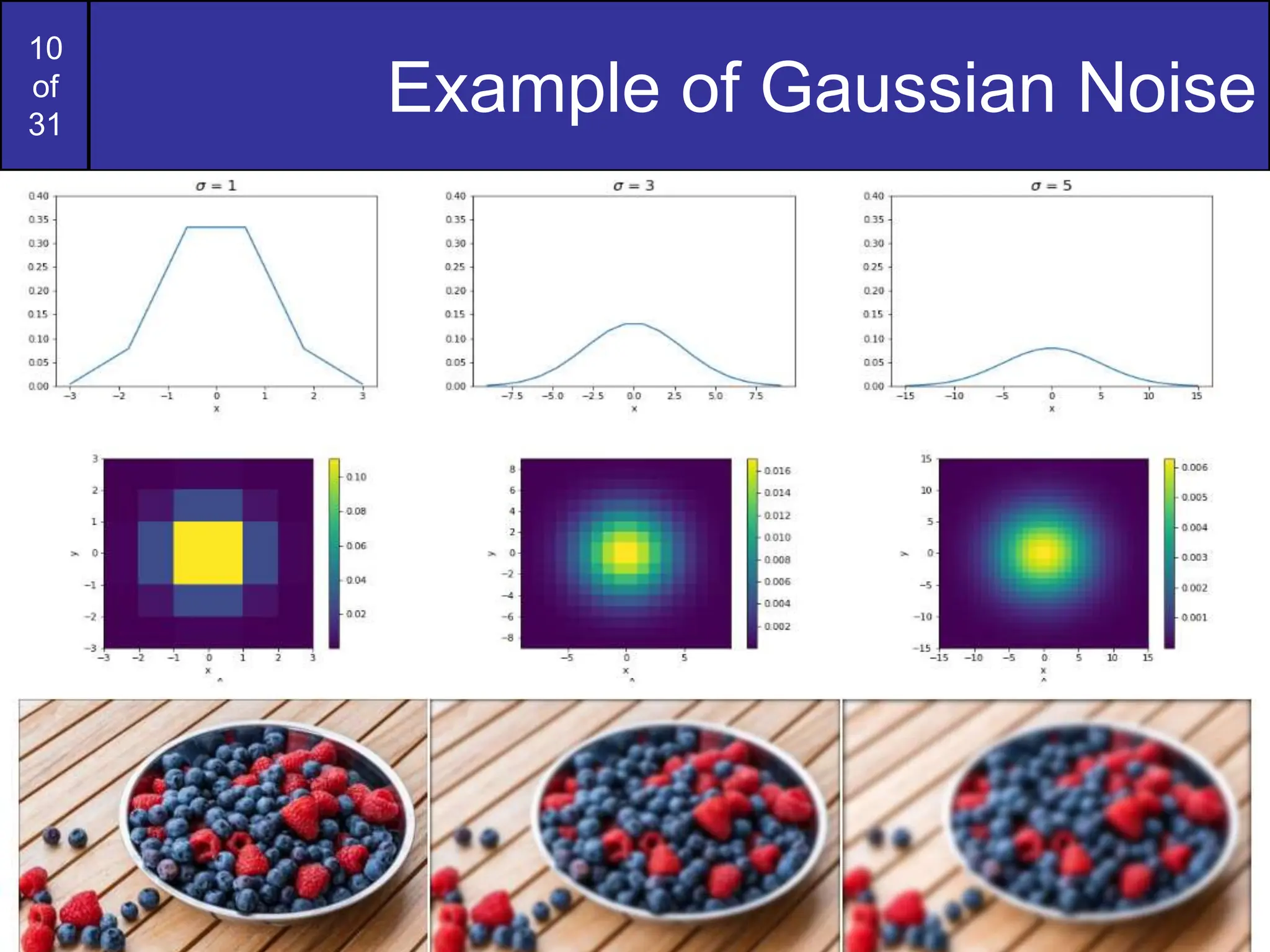
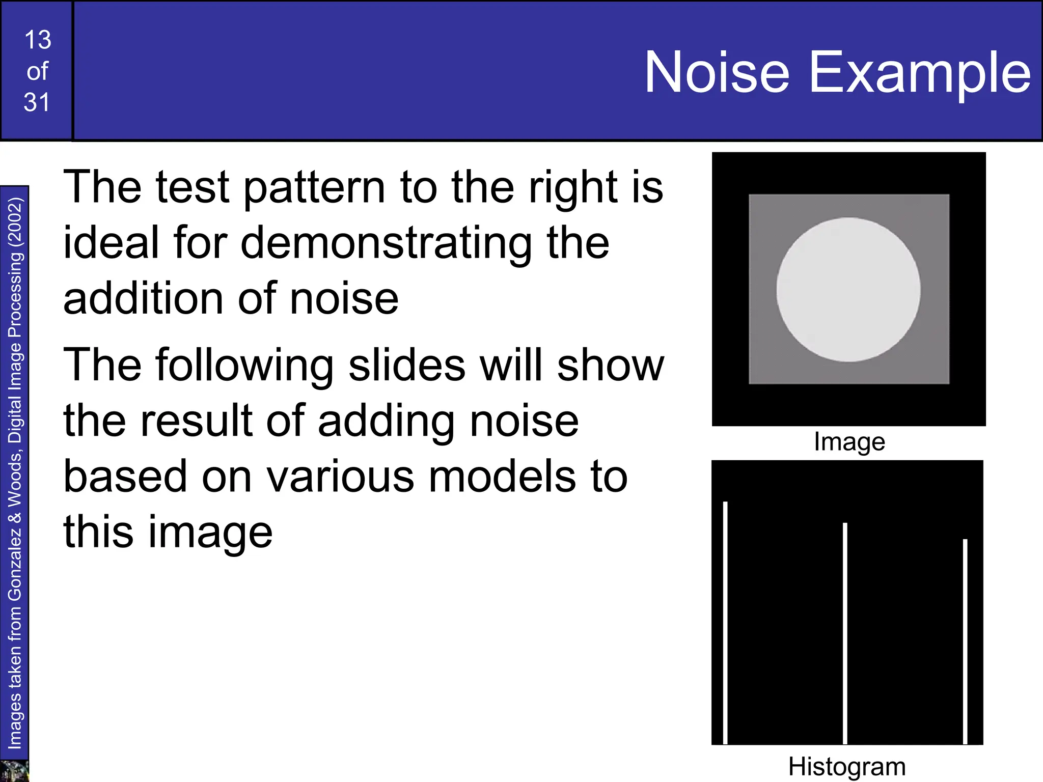
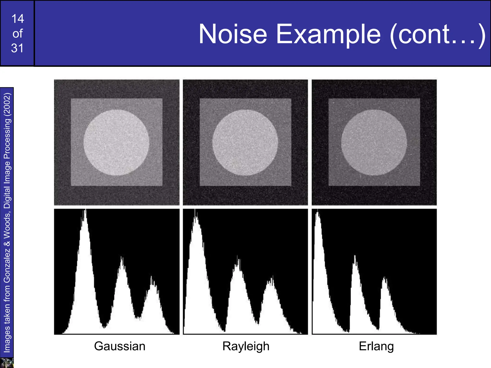
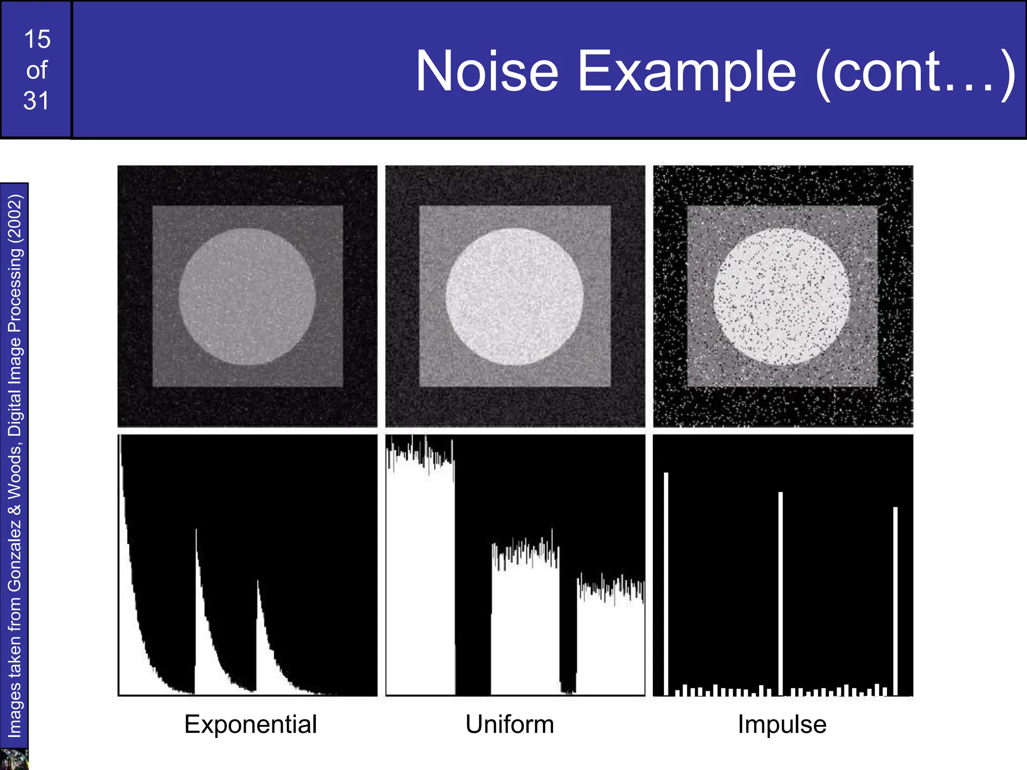
This document covers image restoration techniques focused on noise removal, categorizing noise sources, models, and corresponding removal methods. It discusses spatial and frequency domain techniques, the use of various filters, and the effectiveness of adaptive median filtering for different types of noise. The lecture outlines key principles and examples to illustrate the application of these noise removal methods.

1. Course Website: http://www.comp.dit.ie/bmacnamee
Digital Image Processing
Image Restoration:
Noise Removal

2. 2
of
31
Contents
In this lecture we will look at image
restoration techniques used for noise removal
– What is image restoration?
– Noise and images
– Noise models
– Noise removal using spatial domain filtering
– Periodic noise
– Noise removal using frequency domain
filtering

3. 3
of
31
What is Image Restoration?
Image restoration attempts to restore
images that have been degraded
– Identify the degradation process and attempt
to reverse it
– Similar to image enhancement, but more
objective

4. 4
of
31
Noise and Images
The sources of noise in digital
images arise during image
acquisition (digitization) and
transmission
– Imaging sensors can be
affected by ambient
conditions
– Interference can be added
to an image during
transmission

5. 5
of
31
• Noise can be produced due to different
reasons:
– The image sensor is broken or affected by
external factors;
– Lack of light or overheating of the device at
the moment of taking a photo;
– Interference of the transmission channel, and
so on.

6. 6
of
31
Noise Model
We can consider a noisy image to be
modelled as follows:
where f(x, y) is the original image pixel,
η(x, y) is the noise term and g(x, y) is the
resulting noisy pixel
If we can estimate the model the noise in an
image is based on this will help us to figure
out how to restore the image
)
,
(
)
,
(
)
,
( y
x
y
x
f
y
x
g 



7. 7
of
31
Noise Corruption Example
Noisy Image x
y
Image f (x, y)
54 52 57 55 56 52 51
50 49 51 50 52 53 58
51 51 52 52 56 57 60
48 50 51 49 53 59 63
49 51 52 55 58 64 67
148 154 157 160 163 167 170
151 155 159 162 165 169 172
Original Image x
y
Image f (x, y)

8. 8
of
31

9. 9
of
31
Noise Models
Gaussian Rayleigh
Erlang Exponential
Uniform
Impulse
Images
taken
from
Gonzalez
&
Woods,
Digital
Image
Processing
(2002)
There are many
different models for the
image
noise term η(x, y):
– Gaussian
• Most common model
– Rayleigh
– Erlang
– Exponential
– Uniform
– Impulse
• Salt and pepper
noise

10. 10
of
31
Example of Gaussian Noise

11. 11
of
31
(Cont’d)

12. 12
of
31
• Parameters
• Variance limit - sets the variance range of the noise. The higher the values in the
range, the noisier the image will be. The specified numbers must fall between [0.0,
65025.0];
• Mean - sets the mean of the noise. The higher the mean value, the brighter the
image will be. The specified value must fall between [0.0, 255.0];
• Probability of applying transform - sets the probability of the augmentation being
applied to an image. If you want to apply Gaussian Noise to all images, select a
probability of 1.

13. 13
of
31
Noise Example
The test pattern to the right is
ideal for demonstrating the
addition of noise
The following slides will show
the result of adding noise
based on various models to
this image
Images
taken
from
Gonzalez
&
Woods,
Digital
Image
Processing
(2002)
Histogram to go here
Image
Histogram

14. 14
of
31
Noise Example (cont…)
Images
taken
from
Gonzalez
&
Woods,
Digital
Image
Processing
(2002)
Gaussian Rayleigh Erlang

15. 15
of
31
Noise Example (cont…)
Images
taken
from
Gonzalez
&
Woods,
Digital
Image
Processing
(2002)
Exponential Uniform Impulse
Histogram to go here

16. 16
of
31

17. 17
of
31
Filtering to Remove Noise
We can use spatial filters of different kinds
to remove different kinds of noise
The arithmetic mean filter is a very simple
one and is calculated as follows:
This is implemented as the
simple smoothing filter
Blurs the image to remove
noise



xy
S
t
s
t
s
g
mn
y
x
f
)
,
(
)
,
(
1
)
,
(
ˆ
1/9
1/9
1/9
1/9
1/9
1/9
1/9
1/9
1/9

18. 18
of
31

19. 19
of
31
Noise Removal Example
54 52 57 55 56 52 51
50 49 51 50 52 53 58
51 204 52 52 0 57 60
48 50 51 49 53 59 63
49 51 52 55 58 64 67
148 154 157 160 163 167 170
151 155 159 162 165 169 172
Original Image x
y
Image f (x, y)
Filtered Image x
y
Image f (x, y)

20. 20
of
31
Other Means
There are different kinds of mean filters all of
which exhibit slightly different behaviour:
– Geometric Mean
– Harmonic Mean
– Contraharmonic Mean

21. 21
of
31
Other Means (cont…)
There are other variants on the mean which
can give different performance
Geometric Mean:
Achieves similar smoothing to the arithmetic
mean, but tends to lose less image detail
mn
S
t
s xy
t
s
g
y
x
f
1
)
,
(
)
,
(
)
,
(
ˆ








 


22. 22
of
31
Noise Removal Example
54 52 57 55 56 52 51
50 49 51 50 52 53 58
51 204 52 52 0 57 60
48 50 51 49 53 59 63
49 51 52 55 58 64 67
148 154 157 160 163 167 170
151 155 159 162 165 169 172
Original Image x
y
Image f (x, y)
Filtered Image x
y
Image f (x, y)

23. 23
of
31
Other Means (cont…)
Harmonic Mean:
Works well for salt noise, but fails for pepper
noise
Also does well for other kinds of noise such
as Gaussian noise



xy
S
t
s t
s
g
mn
y
x
f
)
,
( )
,
(
1
)
,
(
ˆ

24. 24
of
31
Noise Corruption Example
54 52 57 55 56 52 51
50 49 51 50 52 53 58
51 204 52 52 0 57 60
48 50 51 49 53 59 63
49 51 52 55 58 64 67
50 54 57 60 63 67 70
51 55 59 62 65 69 72
Original Image x
y
Image f (x, y)
Filtered Image x
y
Image f (x, y)

25. 25
of
31
Other Means (cont…)
Contra harmonic Mean:
Q is the order of the filter and adjusting its
value changes the filter’s behaviour
Positive values of Q eliminate pepper noise
Negative values of Q eliminate salt noise






xy
xy
S
t
s
Q
S
t
s
Q
t
s
g
t
s
g
y
x
f
)
,
(
)
,
(
1
)
,
(
)
,
(
)
,
(
ˆ

26. 26
of
31
Noise Corruption Example
54 52 57 55 56 52 51
50 49 51 50 52 53 58
51 204 52 52 0 57 60
48 50 51 49 53 59 63
49 51 52 55 58 64 67
50 54 57 60 63 67 70
51 55 59 62 65 69 72
Original Image x
y
Image f (x, y)
Filtered Image x
y
Image f (x, y)

27. 27
of
31
Noise Removal Examples
Images
taken
from
Gonzalez
&
Woods,
Digital
Image
Processing
(2002)
Original
Image
Image
Corrupted
By Gaussian
Noise
After A 3*3
Geometric
Mean Filter
After A 3*3
Arithmetic
Mean Filter

28. 28
of
31
Noise Removal Examples (cont…)
Image
Corrupted
By Pepper
Noise
Result of
Filtering Above
With 3*3
Contraharmonic
Q=1.5
Images
taken
from
Gonzalez
&
Woods,
Digital
Image
Processing
(2002)

29. 29
of
31
Noise Removal Examples (cont…)
Images
taken
from
Gonzalez
&
Woods,
Digital
Image
Processing
(2002)
Image
Corrupted
By Salt
Noise
Result of
Filtering Above
With 3*3
Contraharmonic
Q=-1.5

30. 30
of
31
Contraharmonic Filter: Here Be Dragons
Choosing the wrong value for Q when using
the contraharmonic filter can have drastic
results
Images
taken
from
Gonzalez
&
Woods,
Digital
Image
Processing
(2002)

31. 31
of
31
Order Statistics Filters
Spatial filters that are based on ordering the
pixel values that make up the
neighbourhood operated on by the filter
Useful spatial filters include
– Median filter
– Max and min filter
– Midpoint filter
– Alpha trimmed mean filter
Images
taken
from
Gonzalez
&
Woods,
Digital
Image
Processing
(2002)

32. 32
of
31
Median Filter
Median Filter:
Excellent at noise removal, without the
smoothing effects that can occur with other
smoothing filters
Particularly good when salt and pepper
noise is present
)}
,
(
{
)
,
(
ˆ
)
,
(
t
s
g
median
y
x
f
xy
S
t
s 


33. 33
of
31
Noise Corruption Example
54 52 57 55 56 52 51
50 49 51 50 52 53 58
51 204 52 52 0 57 60
48 50 51 49 53 59 63
49 51 52 55 58 64 67
50 54 57 60 63 67 70
51 55 59 62 65 69 72
Original Image x
y
Image f (x, y)
Filtered Image x
y
Image f (x, y)

34. 34
of
31
Max and Min Filter
Max Filter:
Min Filter:
Max filter is good for pepper noise and min
is good for salt noise
)}
,
(
{
max
)
,
(
ˆ
)
,
(
t
s
g
y
x
f
xy
S
t
s 

)}
,
(
{
min
)
,
(
ˆ
)
,
(
t
s
g
y
x
f
xy
S
t
s 


35. 35
of
31
Noise Corruption Example
54 52 57 55 56 52 51
50 49 51 50 52 53 58
51 204 52 52 0 57 60
48 50 51 49 53 59 63
49 51 52 55 58 64 67
50 54 57 60 63 67 70
51 55 59 62 65 69 72
Original Image x
y
Image f (x, y)
Filtered Image x
y
Image f (x, y)

36. 36
of
31
Midpoint Filter
Midpoint Filter:
Good for random Gaussian and uniform
noise





 



)}
,
(
{
min
)}
,
(
{
max
2
1
)
,
(
ˆ
)
,
(
)
,
(
t
s
g
t
s
g
y
x
f
xy
xy S
t
s
S
t
s

37. 37
of
31
Noise Corruption Example
54 52 57 55 56 52 51
50 49 51 50 52 53 58
51 204 52 52 0 57 60
48 50 51 49 53 59 63
49 51 52 55 58 64 67
50 54 57 60 63 67 70
51 55 59 62 65 69 72
Original Image x
y
Image f (x, y)
Filtered Image x
y
Image f (x, y)

38. 38
of
31
Alpha-Trimmed Mean Filter
Alpha-Trimmed Mean Filter:
We can delete the d/2 lowest and d/2 highest grey
levels
So gr(s, t) represents the remaining mn – d pixels
Use for multiple types of noise.
If d==0 : Arithmetic mean filter
If d==mn-1 : Median Filter.




xy
S
t
s
r t
s
g
d
mn
y
x
f
)
,
(
)
,
(
1
)
,
(
ˆ

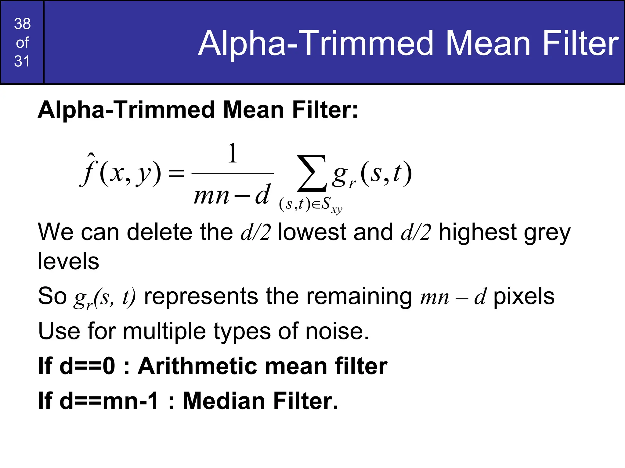
39. 39
of
31
Problem:
4 0 4 9
4 1 8 8
1 1 6 6
1 0 5 6
1 1 5 6
Order: 5*4
M=5
N=4
Mn = 5*4 = 20
Assume d = mn-2
= 20-2 = 18
Alpha = d/2 = 18/2 = 9
0, 0, 1, 1, 1, 1, 1, 1, 4, 4, 4, 5, 5, 6, 6, 6, 6, 8, 8, 9
= 1/(20 - 18) [4+4] = ½(8) = 4 .




xy
S
t
s
r t
s
g
d
mn
y
x
f
)
,
(
)
,
(
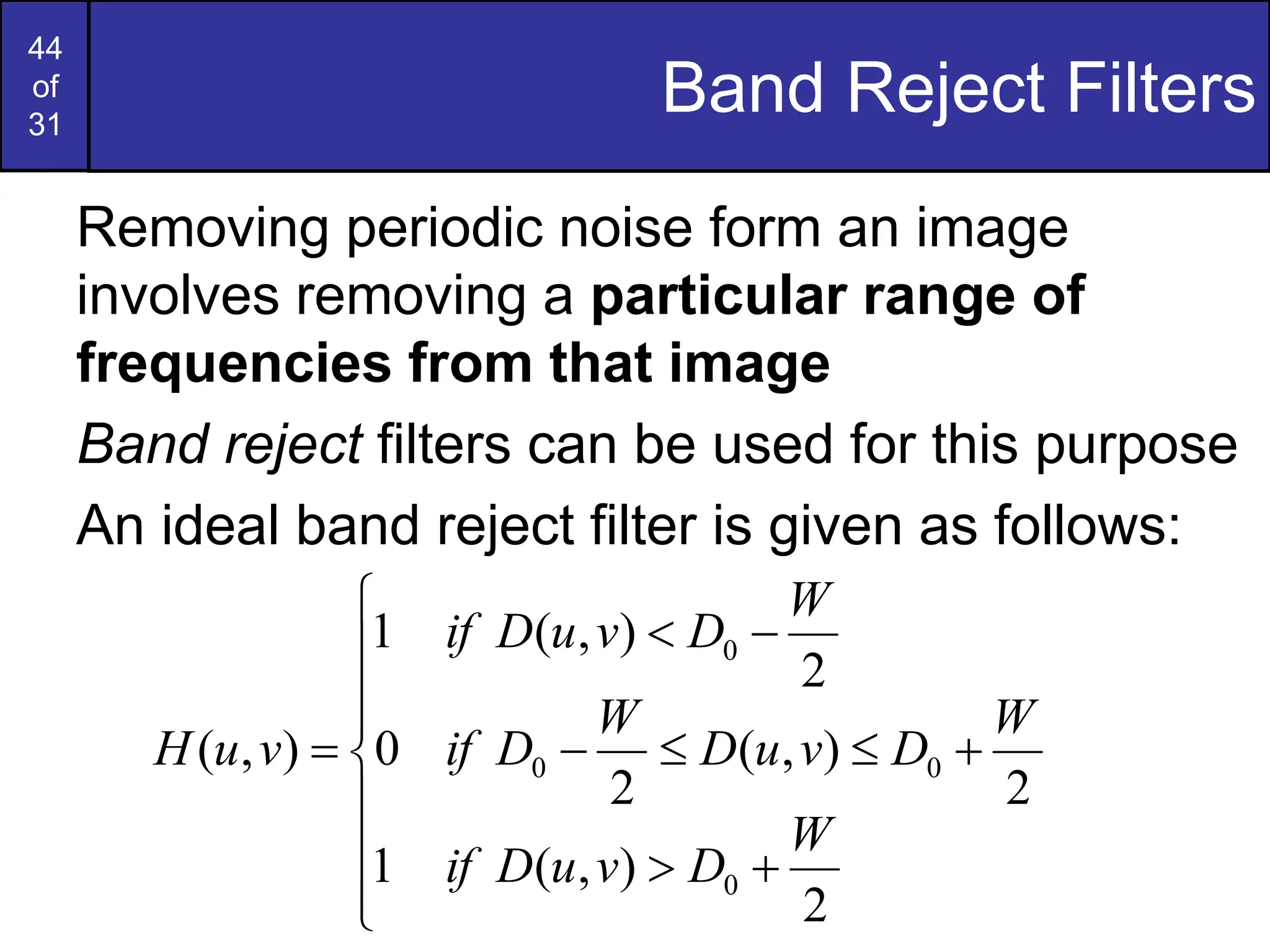
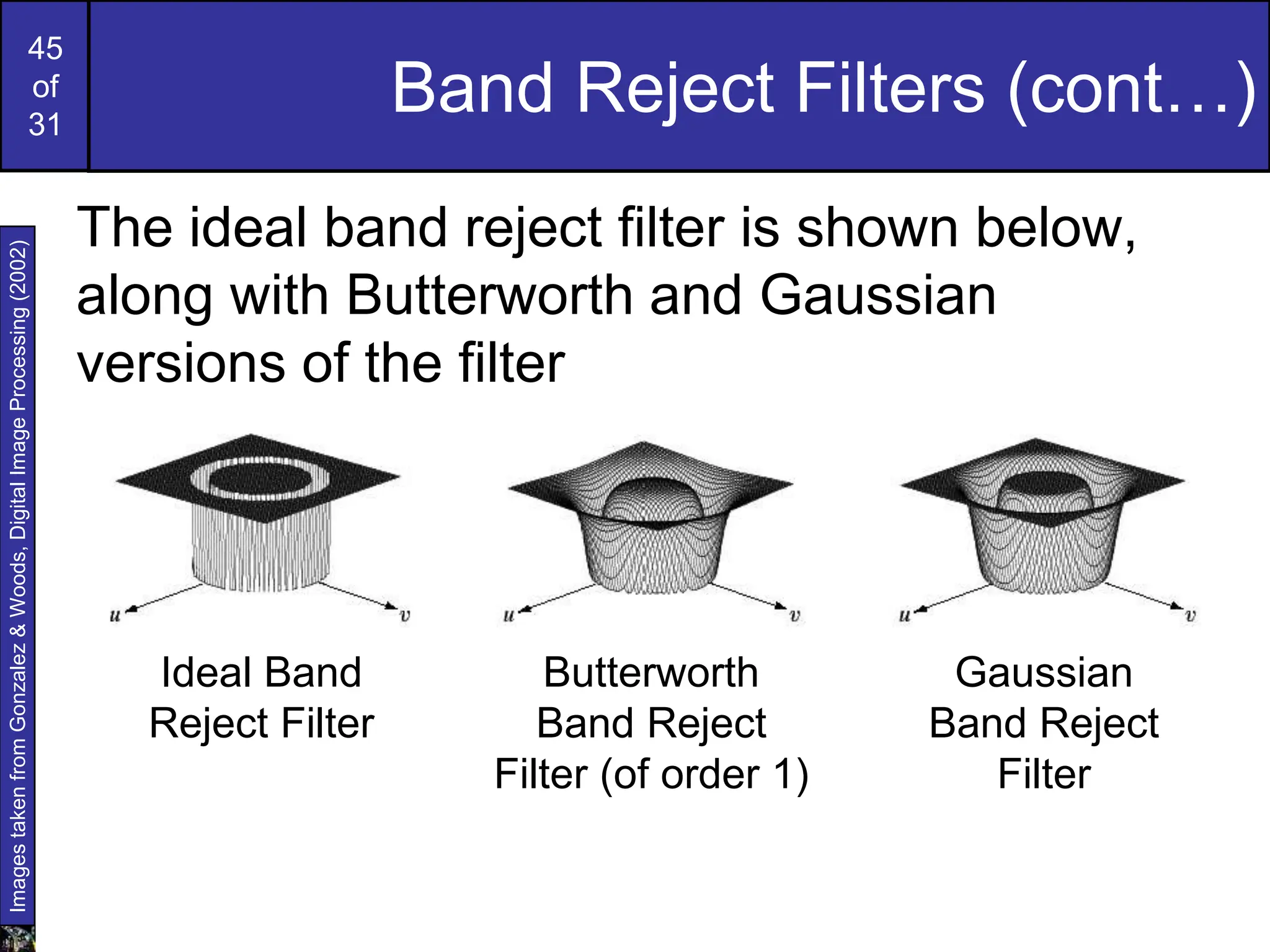
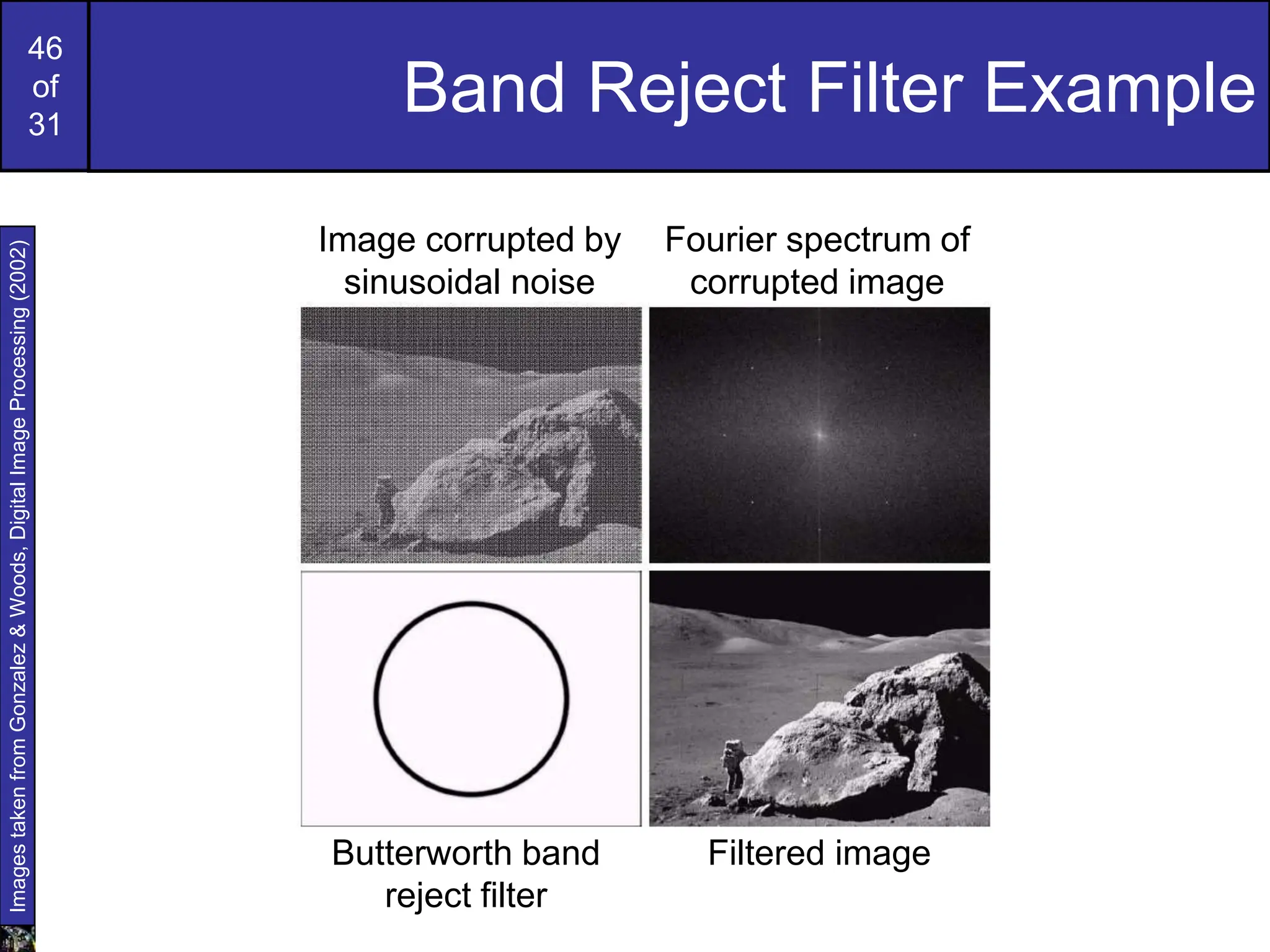
1
)
,
(
ˆ

40. 40
of
31
Noise Removal Examples
Images
taken
from
Gonzalez
&
Woods,
Digital
Image
Processing
(2002)
Image
Corrupted
By Salt And
Pepper Noise
Result of 1
Pass With A
3*3 Median
Filter
Result of 2
Passes With
A 3*3 Median
Filter
Result of 3
Passes With
A 3*3 Median
Filter

41. 41
of
31
Noise Removal Examples (cont…)
Images
taken
from
Gonzalez
&
Woods,
Digital
Image
Processing
(2002)
Image
Corrupted
By Pepper
Noise
Image
Corrupted
By Salt
Noise
Result Of
Filtering
Above
With A 3*3
Min Filter
Result Of
Filtering
Above
With A 3*3
Max Filter

42. 42
of
31
Noise Removal Examples (cont…)
Images
taken
from
Gonzalez
&
Woods,
Digital
Image
Processing
(2002)
Image
Corrupted
By Uniform
Noise
Image Further
Corrupted
By Salt and
Pepper Noise
Filtered By
5*5 Arithmetic
Mean Filter
Filtered By
5*5 Median
Filter
Filtered By
5*5 Geometric
Mean Filter
Filtered By
5*5 Alpha-Trimmed
Mean Filter

43. 43
of
31
Periodic Noise
Typically arises due to
electrical or electromagnetic
interference.
Repeating pattern has been
added on top of the original
image.
Gives rise to regular noise
patterns in an image
Frequency domain techniques
in the Fourier domain are most
effective at removing periodic
noise
Images
taken
from
Gonzalez
&
Woods,
Digital
Image
Processing
(2002)

44. 44
of
31
Band Reject Filters
Removing periodic noise form an image
involves removing a particular range of
frequencies from that image
Band reject filters can be used for this purpose
An ideal band reject filter is given as follows:


















2
)
,
(
1
2
)
,
(
2
0
2
)
,
(
1
)
,
(
0
0
0
0
W
D
v
u
D
if
W
D
v
u
D
W
D
if
W
D
v
u
D
if
v
u
H

45. 45
of
31
Band Reject Filters (cont…)
The ideal band reject filter is shown below,
along with Butterworth and Gaussian
versions of the filter
Images
taken
from
Gonzalez
&
Woods,
Digital
Image
Processing
(2002)
Ideal Band
Reject Filter
Butterworth
Band Reject
Filter (of order 1)
Gaussian
Band Reject
Filter

46. 46
of
31
Band Reject Filter Example
Images
taken
from
Gonzalez
&
Woods,
Digital
Image
Processing
(2002)
Image corrupted by
sinusoidal noise
Fourier spectrum of
corrupted image
Butterworth band
reject filter
Filtered image

47. 47
of
31
Summary
In this lecture we will look at image restoration
for noise removal
Restoration is slightly more objective than
enhancement
Spatial domain techniques are particularly
useful for removing random noise
Frequency domain techniques are particularly
useful for removing periodic noise

48. 48
of
31
Adaptive Filters
The filters discussed so far are applied to an
entire image without any regard for how
image characteristics vary from one point to
another
The behaviour of adaptive filters changes
depending on the characteristics of the
image inside the filter region
We will take a look at the adaptive median
filter

49. 49
of
31
Adaptive Median Filtering
The median filter performs relatively well on
impulse noise as long as the spatial density
of the impulse noise is not large
The adaptive median filter can handle much
more spatially dense impulse noise, and
also performs some smoothing for non-
impulse noise
The key insight in the adaptive median filter
is that the filter size changes depending on
the characteristics of the image

50. 50
of
31
Adaptive Median Filtering (cont…)
Remember that filtering looks at each
original pixel image in turn and generates a
new filtered pixel
First examine the following notation:
– zmin = minimum grey level in Sxy
– zmax = maximum grey level in Sxy
– zmed = median of grey levels in Sxy
– zxy = grey level at coordinates (x, y)
– Smax =maximum allowed size of Sxy

51. 51
of
31
Adaptive Median Filtering (cont…)
Level A: A1 = zmed – zmin
A2 = zmed – zmax
If A1 > 0 and A2 < 0, Go to level B
Else increase the window size
If window size ≤ repeat Smax level A
Else output zmed
Level B: B1 = zxy – zmin
B2 = zxy – zmax
If B1 > 0 and B2 < 0, output zxy
Else output zmed

52. 52
of
31
Adaptive Median Filtering (cont…)
The key to understanding the algorithm is to
remember that the adaptive median filter
has three purposes:
– Remove impulse noise
– Provide smoothing of other noise
– Reduce distortion

53. 53
of
31
Adaptive Filtering Example
Images
taken
from
Gonzalez
&
Woods,
Digital
Image
Processing
(2002)
Image corrupted by salt
and pepper noise with
probabilities Pa = Pb=0.25
Result of filtering with a 7
* 7 median filter
Result of adaptive
median filtering with i = 7