머신러닝분야에서 활용되는 자연어 처리기술에 대한 전반적 소개(I)

1. 머신러닝의 자연어 처리기술(I)
2016. 7.
김홍배
“言語と画像の表現学習“, 慶應義塾大学, 野口裕貴
“Word2vec from scratch”, KAIST, 이진표
1

2. 1. 개요
2. 분산표현의 개요
3. 자연어처리의 개요
4. 언어의 벡터표현
5. encoder-decoder 모델
6. 멀티모달모델
목차
2

3. 사진으로 연애이야기를 만드는 AI
「회의마지막에우리들은긴장된분위기였다. 그리고나는친구를쳐다봤다.
물론나는그가가도록놔둘의도는없었다. 달리할말을모르겠지만,
그는가장아름다운 남자다」
3

4. Neural Storyteller에서 사용되는 기술
단어
표현
문장과
사진의 결합
사진으로부터
설명문을 작성
Kiros 2015.11
뉴럴넷（NN）이 기반
[Mikolov+ 13] [Kiros+ 15]
[Kiros+ 14]문장
표현
사진
표현
4

5. 오늘의 주제
• NN이 파워풀한 이유중 하나：분산표현
• NN에 언어 및 사진을 학습시키는 방법
5

6. 분산표현 [Hinton+ 1986]
분산표현
1986년、Geoffrey Hinton이 뉴론이 어떻게 개념을
나 타 내 는 가 를 설 명 하 기 위 해 서 분 산 표 현
(distributed representation)을 제안
6

7. 목차
1. 개요
2. 분산표현의 개요
3. 자연어처리의 개요
4. 언어의 벡터표현
5. encoder-decoder 모델
6. 멀티모달모델
7

8. 국소표현 vs 분산표현
8

9. 국소표현
1개 뉴론의 작동으로 1개의 개념을 나타냄
벡터형태로 나타내서 one-hot vector
[1, 0, 0, 0, 0]
[0, 1, 0, 0, 0]
[0, 0, 1, 0, 0]
...
...
9

10. 분산표현
복수 뉴론의 작동으로 1개의 개념을 나타냄.
[0.5, 0.0, 1.0, 1.0, 0.3]
[0.5, 0.0, 1.0, 1.0, 0.0]
[0.2, 0.9, 0.5, 0.0, 1.0]
...
... 10

11. 분산표현
개념을 특징의 조합으로 나타냄.
＝ 1·펫 + 1 · 멍멍 + 0 · 야옹 + 0.1 · 타는것 + 0.1 · 바다
＝ 1·펫 + 0 · 멍멍 + 1 · 야옹 + 0 .0· 타는것 + 0 · 바다
＝ 0·펫 + 0 · 멍멍 + 0 · 야옹 + 0.9 · 타는것 + 0.8 · 바다
특징
계수
11

12. 개념의 유사
국소표현 분산표현
비슷하다！
전혀 다름
12

13. 문자인식의 분산표현
...+ 0.9 + 0.1
...+ 0.5 + 0.6
≈ 0.8
계수
≈ 0.7
특징
13

14. 딥뉴럴네트웍
음성인식과 사진인식을 시작으로 다양한 분야에서
성과를 만들어내고 있다.
최근에는 자연어처리에도 활용되고 있다.
14

15. 1. 개요
2. 분산표현의 개요
3. 자연어처리의 개요
4. 언어의 벡터표현
5. encoder-decoder 모델
6. 멀티모달모델
목차
15

16. 자연어처리（NLP）
컴퓨터과학, 인공지능과 언어학이 합쳐진 분야
컴퓨터 과학 인공지능
자연어처리
언어학
16

17. 자연어 처리 업무
쉬움 중간 어려움
• 스펠링 체크
• 키워드 검사
• 유사어 감지
• 웹사이트 및 서류의
형태 해석
• 구문해석 etc.
• 기계번역
• 감정분석
• 질의응답시스템
17

18. 기계번역
문구기반 번역의 예
He threw the ball
단어의 모호성
그는 던졌다 볼을
그는 볼을 던졌다
18

19. 감정분석
문장으로부터 감정을 판단
「매우 재밌다. 아무리 놀아도 실증나지않는다.」
→ 0.86
「설치하지마. 데이터만 낭비한다.」
→ -0.68
긍정적
부정적
19

20. 질문응답시스템(QA 시스템）
closed-domain – 정해진 분야의 질문에 응답
「라마는 무슨 과？」 → 「낙타과」
open-domain – 어떠한 질문에도 응답
「왜 나는 결혼을 못하나 ?」 → 「...」
20

21. 자연어 처리의 어려움
언어・상황・환경・지각 지식의 학습 및 표현의 복잡함
→ Rule 기반만으로는 무리인가 ？
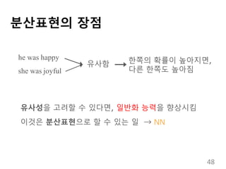
DNN은 분산표현의 장점으로 인해
모호하지만 풍부한 정보를 얻을 수 있다.
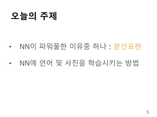
→ 단어의 벡터화로부터 시작
21

22. 1. 개요
2. 분산표현의 개요
3. 자연어처리의 개요
4. 언어의 벡터표현
5. encoder-decoder 모델
6. 멀티모달모델
목차
22

23. 단어의 국소표현
[1, 0, 0, 0, 0]
[0, 1, 0, 0, 0]
[0, 0, 1, 0, 0]
...
고양이
개
사람
이것만 가지고는 단어의 의미를 전혀 알 수 없다.
→ 단어의 의미를 파악하는 벡터를 갖고 싶다.
...
23

24. 분포가설 [Harris 1954, Firth 1957]
“You shall know a word by the company it keeps”
- J. R. Firth
비슷한 문맥을 가진 단어는 비슷한 의미를 갖는다.
현대의 통계적 자연어 처리에서 획기적인 발상
24

25. Count-based vs Predictive methods
분포가설에 기반한 방법은 크게 2종류로 나눈다.
• count-based methods
• 예：SVD (LSA)、HAL、etc.
• 단어, 문맥 출현횟수를 세는 방법
• predictive methods
 예：NPLM、word2vec、etc.
 단어에서 문맥 또는 문맥에서 단어를 예측하는 방법
25

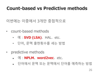
26. 이번에는 이중에서 3개만 중점적으로
• count-based methods
• 예：SVD (LSA)、HAL、etc.
• 단어, 문맥 출현횟수를 세는 방법
• predictive methods
 예：NPLM、word2vec、etc.
 단어에서 문맥 또는 문맥에서 단어를 예측하는 방법
Count-based vs Predictive methods
26

27. 문맥(context)의 정의
• 문맥창(다음 슬라이드)
• 자신 이외의 ○○중에 나타나는 단어
• 문장
• 단락
• 문서
27

28. 문맥창
크기 2k+1의 단어열에 대해
기준단어(April)주변의 단어가 문맥
k＝4 의 예
It was a bright cold day in April, and the clocks were strikingthirteen.
전 4 단어 후 4 단어
기준
문맥
28

29. 단어문맥행렬(co-occurance matrix）
예：k=1 의
문맥창으로 한 경우
|V| 는 어휘수
I enjoy technology.
I like eating.
I like to sleep.
I enjoy technology like eating to sleep .
I 0 1 0 2 0 0 0 0
enjoy 1 0 1 0 0 0 0 0
technology 0 1 0 0 0 0 0 1
like 2 0 0 0 1 1 0 0
eating 0 0 0 1 0 0 0 1
to 0 0 0 1 0 0 1 0
sleep 0 0 0 0 0 1 0 1
. 0 0 1 0 1 0 1 0
|V|
|V|
“like” 앞에 “I”가 두번 출현
“like” 뒤에 “eating”이 한번 출현
29

30. 단어문맥행렬
각행을 단어벡터로 사용
그러나 단어가 많아지면,
벡터도 커진다(수십만 차원도 됨)
technology 0 1 0 0 0 0 0 1
like 2 0 0 0 1 1 0 0
eating 0 0 0 1 0 0 0 1
어휘수
30

31. 조밀한 벡터
고차원 벡터의「가장 중요한 정보」를 유지하면서
저차원・조밀한 벡터로 압축하고 싶다.
(e.g. 수십만 차원 → 수백 차원)
→ 특이치분해（Singular Value Decomposition, SVD)
31

32. 특이치분해（SVD）
X U VT
단어문맥행렬
각열은 XXT 의
고유벡터
각행은 XTX 의
고유벡터
대각선 값은 XXT 와 XTX 의 고유치
(크기순)
대응하는 고유치
의 크기순으로
나열됨.
|V|
|V|
Σ
𝝈 𝟏
𝝈 𝟐
⋱
𝝈 𝒏
𝝈 𝟏>𝝈 𝟐> ….. >𝝈 𝒏
∑ = 앞쪽이 중요하고
뒤로 갈 수록 중요도가 낮아짐 32

33. 단어벡터
- U 의 각행을 단어벡터로 사용하되
- 중요도가 높은 앞쪽 고유치(N개)에 해당하는
U 의 앞쪽 N열까지 사용
U
단어벡터
사용하지않음
N
33

34. 처음 2열까지 가시화 예
x y
-0.5 0.6
-0.6 -0.6
-0.2 -0.2
U
like
I
enjoy
단어벡터
단어벡터
34

35. K = 2 K = 3
단어벡터 예
35

36. 좀더 본격적으로
다음은 Brown Corpus 를 사용해보자
• 단어수：약 100만
• 어휘수：공간으로 나눈 결과, 약 8만
• 우선 단어문맥행렬을 만들어 보려는데….
36

37. 어휘수 줄이기
단어문맥행렬이 너무 크다
(어휘수 8만 → 80,000x80,000）
→ 발생빈도로 1,000번 이하의 단어를 정리
(어휘수 1,000 → 행렬 1,001x1,001）
37

38. 단어벡터의 가시화
100차원의 벡터
(U의 100열까지 사용)
38

39. 유사한(similarity, correlation, 관련성) 단어
유사도＝
w1과 w2가 유사하면  1
w1과 w2가 관련없으면  0
39

40. 계산량 문제
새로운 텍스트 데이터를 사용할 경우,
단어문맥 행렬을 새롭게 만들어 SVD을 다시 계산
SVD 계산량은 n×m행렬의 경우, O(mn2) (n < m)
→ 즉 어휘수에 한계
실제 어휘수를 늘려본 결과
100000
몇일 소요
40

41. 뉴럴 확률 언어 모델 [Bengio+ 2003]
NN으로 만들어내는 언어모델
→ 언어모델은 또 뭐야 ?
41

42. 언어모델
단어열의 문법과 의미가 올바른 정도를 나타내는 확률을 계산하는 모델
PLM(밥을 먹다) > PLM(먹다 밥을)
응용예 : 단어입력, 스펠링 체크, 기계번역 및 음성인식에 있어서 복수 문
장후보의 평가에 사용
우리 인류의 궁극적인 꿈
0.023%
우리 여기에 공급적인 com
0.002%
?
음성인식의 예
김성훈 교수님 강의 중
42

43. n-gram 언어모델
계산량의 한계로 조건을 붙여 확률을 근사화
어떤 단어의 출현확률은 이전 (n-1)개의 단어에 의존한다.
n=4 의경우
...man stood still as they slowly walked through the...
이것을 n-1차 마코프 과정이라고 함.
조건
43

44. n-gram 언어모델
unigram（n=1）
P(He plays tennis.)=P(He)*P(plays)*P(tennis)*P(.)
bigram（n=2）
P(He plays tennis.) = P(He)*P(plays|He)*P(tennis|plays)*P(.|tennis)
trigram（n=3）
P(He plays tennis.) = P(He)*P(plays|He)*P(tennis|He plays)*P(.|plays tennis)
...
순서를 전혀 고려하지 않음
44

45. n-gram로 언어모델링
이와 같이 n-gram의 n을 증가시킨다.
n 을 증가시켜도, 데이터가 충분하면 성능은 좋아진다.
그러나 단어가 가질 수 있는 조합이 |V|n 로 지수적으로 커진다.
→ 지수적으로 학습데이터가 필요해짐.
45

46. n-gram에 있어서 문제점
Brown Corpus를 3-gram으로 언어모델을 만들어보면
“he was happy”는 6건 나옴
46

47. “she was joyful”은 “0”
→ n-gram 모델이라면 확률 0%
→ Smoothing 등의 처리를 하는 경우가 있음.
그러나 문제는 완전히 해결되지 않음.
간단한 예
（add-one smoothing）
n-gram에 있어서 문제점
47

48. 분산표현의 장점
유사성을 고려할 수 있다면, 일반화 능력을 향상시킴
이것은 분산표현으로 할 수 있는 일 → NN
유사함
he was happy
she was joyful
한쪽의 확률이 높아지면,
다른 한쪽도 높아짐
48

49. 임베드행렬(embedding matrix）
이행렬을 NN으로 훈련시키면 ?
i 행렬이
단어 i 의 백터
단어벡터(임베드 벡터)의 집합
|V|
m 은 임베드벡터의 크기
(임의값)
m
49

50. 뉴럴 확률언어모델(NPLM)
단어열로부터 다음 단어를 예측
（e.g. Apples are ）
50

51. NPLM과 단어벡터
NPLM의 임베드행렬 C의 각행을 단어벡터로서 사용
그러나, NPLM의 첫번째 목적은 언어 모델
단어벡터는 부산물
단어벡터를 얻어내는 것에 적합한 방법이 있다면 ?
51

52. word2vec [Mikolov+ 2013]
CBOW（연속 bag-of-words）모델
• 문맥으로부터 단어를 예측
• 소규모 데이터 셋에 대하여 성능이 좋음
skip-gram 모델
• 단어로부터 문맥을 예측
• 대규모 데이터 셋에 사용됨
skip-gram은 성능이 좋고 빨라서 인기
52

53. CBOW (Original)
• Continuous-Bag-of-word model
• Idea: Using context words, we can predict center word
i.e. Probability( “It is ( ? ) to finish”  “time” )
• Present word as distributed vector of probability  Low dimension
• Goal: Train weight-matrix(W ) satisfies below
• Loss-function (using cross-entropy method)
argmax 𝑊 {𝑀𝑖𝑛𝑖𝑚𝑖𝑧𝑒 𝒕𝒊𝒎𝒆 − 𝑠𝑜𝑓𝑡𝑚𝑎𝑥 𝑝𝑟 time 𝒊𝒕, 𝒊𝒔, 𝒕𝒐, 𝒇𝒊𝒏𝒊𝒔𝒉 ; 𝑊 }
* Softmax(): K-dim vector of x∈ℝ  K-dim vector that has (0,1)∈ℝ
𝐸 = − log 𝑝(𝑤𝑡|𝑤𝑡−𝐶.. 𝑤𝑡+𝐶)
context words (window_size=2)
53

54. CBOW (Original)
• Continuous-Bag-of-word model
• Input
• “one-hot” word vector
• Remove nonlinear hidden layer
• Back-propagate error from
output layer to Weight matrix
(Adjust W s)
It
is
finish
to
time
[
0
1
0
0
0
]
Wout T∙h =
𝒚(predicted)
[0 0 1 0 0]T
Win
∙
h
Win ∙ x i
[0 0 0 0 1]T
Win
∙
y(true) =
Backpropagate to
Minimize error
vs
Win(old) Wout(old)
Win(new) Wout(new)
Win, Wout ∈ ℝ 𝑛×|𝑉|: Input, output Weight
-matrix, n is dimension for word embedding
x 𝑖, 𝑦 𝑖: input, output word vector
(one-hot) from vocabulary V
ℎ: hidden vector, avg of W*x
[NxV]*[Vx1]  [Nx1] [VxN]*[Nx1]  [Vx1]
Initial input, not results
54

55. • Skip-gram model
• Idea: With center word,
we can predict context words
• Mirror of CBOW (vice versa)
i.e. Probability( “time”  “It is ( ? ) to finish” )
• Loss-function:
Skip-Gram (Original)
𝐸 = − log 𝑝(𝑤𝑡−𝐶. . 𝑤𝑡+𝐶|𝑤𝑡)
time
It
is
to
finish
Win ∙ x i
h
y i
Win(old) Wout(old)
Win(new) Wout(new)
[NxV]*[Vx1]  [Nx1] [VxN]*[Nx1]  [Vx1]
CBOW: 𝐸 = − log 𝑝(𝑤𝑡|𝑤𝑡−𝐶.. 𝑤𝑡+𝐶)
55

56. • Hierarchical Soft-max function
• To train weight matrix in every step, we need to pass the
calculated vector into Loss-Function
• Soft-max function
• Before calculate loss function
calculated vector should normalized as real-number in
(0,1)
Extension of Skip-Gram(1)
𝑻: 𝑤ℎ𝑜𝑙𝑒 𝑠𝑡𝑒𝑝
𝒄: 𝑠𝑖𝑧𝑒 𝑜𝑓 𝑡𝑟𝑎𝑖𝑛𝑖𝑛𝑔 𝑐𝑜𝑛𝑡𝑒𝑥𝑡 𝑤𝑖𝑛𝑑𝑜𝑤
𝒘 𝒕, 𝒘 𝒕+𝒋: 𝑐𝑢𝑟𝑒𝑛𝑡 𝑠𝑡𝑒𝑝′ 𝑠 𝑤𝑜𝑟𝑑 𝑎𝑛𝑑 𝑗 − 𝑡ℎ 𝑤𝑜𝑟𝑑 𝒘𝒕
(𝑬 = − 𝐥𝐨𝐠 𝒑 𝒘 𝒕−𝑪. . 𝒘 𝒕+𝑪 𝒘 𝒕 )
56

57. • Hierarchical Soft-max function (cont.)
• Soft-max function
(I have already calculated, it’s boring …….…)
Extension of Skip-Gram(1)
Original soft-max function
of skip-gram model
57

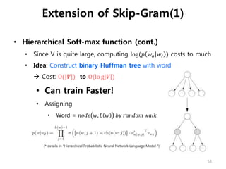
58. • Hierarchical Soft-max function (cont.)
• Since V is quite large, computing log(𝑝 𝑤𝑜 𝑤𝐼 ) costs to much
• Idea: Construct binary Huffman tree with word
 Cost: O( 𝑽 ) to O(lo g 𝑽 )
• Can train Faster!
• Assigning
• Word = 𝑛𝑜𝑑𝑒 𝑤, 𝐿 𝑤 𝑏𝑦 𝑟𝑎𝑛𝑑𝑜𝑚 𝑤𝑎𝑙𝑘
(* details in “Hierarchical Probabilistic Neural Network Language Model ")
Extension of Skip-Gram(1)
58

59. • Negative Sampling (similar to NCE)
• Size(Vocabulary) is computationally huge!  Slow for train
• Idea: Just sample several negative examples!
• Do not loop full vocabulary, only use neg. sample  fast
• Change the target word as negative sample and learn
negative examples  get more accuracy
• Objective function
Extension of Skip-Gram(2)
i.e. “Stock boil fish is toy” ????  negative sample
Noise Constrastive Estimation
𝐸 = − log 𝑝(𝑤𝑡−𝐶. . 𝑤𝑡+𝐶|𝑤𝑡)
59

60. • Subsampling
• (“Korea”, ”Seoul”) is helpful, but (“Korea”, ”the”) isn’t helpful
• Idea: Frequent word vectors (i.e. “the”) should not change
significantly after training on several million examples.
• Each word 𝑤𝑖 in the training set is discarded with below
probability
• It aggressively subsamples frequent words while preserve
ranking of the frequencies
• But, this formula was chosen heuristically…
Extension of Skip-Gram(3)
f wi : 𝑓𝑟𝑒𝑞𝑢𝑛𝑐𝑦 𝑜𝑓 𝑤𝑜𝑟𝑑 𝑤𝑖
𝑡: 𝑐ℎ𝑜𝑠𝑒𝑛 𝑡ℎ𝑟𝑒𝑠ℎ𝑜𝑙𝑑, 𝑎𝑟𝑜𝑢𝑛𝑑 10−5
60

61. • Evaluation
• Task: Analogical reasoning
• Accuracy test using cosine similarity determine how the model
answer correctly.
i.e. vec(X) = vec(“Berlin”) – vec(“Germany”) + vec(“France”)
Accuracy = cosine_similarity( vec(X), vec(“Paris”) )
• Model: skip-gram model(Word-embedding dimension = 300)
• Data Set: News article (Google dataset with 1 billion words)
• Comparing Method (w/ or w/o 10-5subsampling)
• NEG(Negative Sampling)-5, 15
• Hierarchical Softmax-Huffman
• NCE-5(Noise Contrastive Estimation)
Extension of Skip-Gram
61

62. • Empirical Results
• Model w/ NEG outperforms the HS on the analogical reasoning task
(even slightly better than NCE)
• The subsampling improves the training speed several times and
makes the word representations more accurate
Extension of Skip-Gram
62

63. • Word base model can not represent idiomatic word
• i.e. “Newyork Times”, “Larry Page”
• Simple data driven approach
• If phrases are formed based on 1-gram, 2-gram counts
• Target words that has high score would meaningful phrase
Learning Phrases
𝛿: 𝑑𝑖𝑠𝑐𝑜𝑢𝑛𝑡𝑖𝑛𝑔 𝑐𝑜𝑒𝑓𝑓𝑖𝑐𝑖𝑒𝑛𝑡
(P𝑟𝑒𝑣𝑒𝑛𝑡 𝑡𝑜𝑜 𝑚𝑎𝑛𝑦 𝑝ℎ𝑟𝑎𝑠𝑒𝑠 𝑐𝑜𝑛𝑠𝑖𝑠𝑡𝑖𝑛𝑔 𝑜𝑓 𝑖𝑛𝑓𝑟𝑒𝑞𝑢𝑒𝑛𝑡 𝑤𝑜𝑟𝑑𝑠)
63

64. • Evaluation
• Task: Analogical reasoning
• Accuracy test using cosine similarity determine how the model
answer correctly with phrase
• i.e. vec(X) = vec(“Steve Ballmer”) – vec(“Microsoft”) + vec(“Larry Page”)
Accuracy = cosine_similarity( vec(x), vec(“Google”) )
• Model: skip-gram model(Word-embedding dimension = 300)
• Data Set: News article (Google dataset with 1 billion words)
• Comparing Method (w/ or w/o 10-5subsampling)
• NEG-5
• NEG-15
• HS-Huffman
Learning Phrases
64

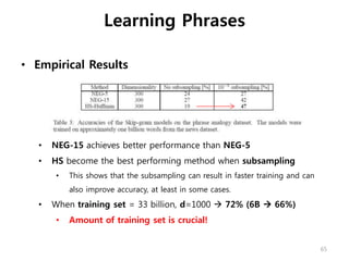
65. • Empirical Results
• NEG-15 achieves better performance than NEG-5
• HS become the best performing method when subsampling
• This shows that the subsampling can result in faster training and can
also improve accuracy, at least in some cases.
• When training set = 33 billion, d=1000  72% (6B  66%)
• Amount of training set is crucial!
Learning Phrases
65

66. • Simple vector addition (on Skip-gram model)
• Previous experiments shows Analogical reasoning (A+B-C)
• Vector’s values are related logarithmically to the probabilities
 Sum of two vector is related to product of context distribution
• Interesting!
Additive Compositionality
66

67. • Contributions
• Showed detailed process of training distributed
representation of words and phrases
• Can be more accurate and faster model than previous
word2vec model by sub-sampling
• Negative Sampling: Extremely simple and accurate for
frequent words. (not frequent like phrase, HS was better)
• Word vectors can be meaningful by simple vector
addition
• Made a code and dataset as open-source project
Conclusion
67

68. • Compare to other Neural network model
<Find most similar word>
• Skip-gram model trained on large corpus outperforms all
to other paper’s models.
Conclusion
68