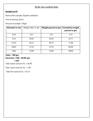
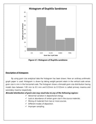
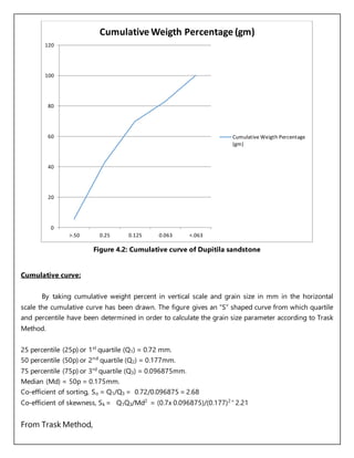
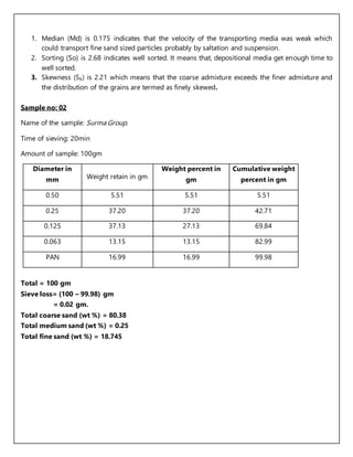
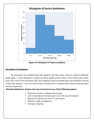
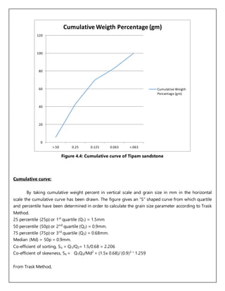
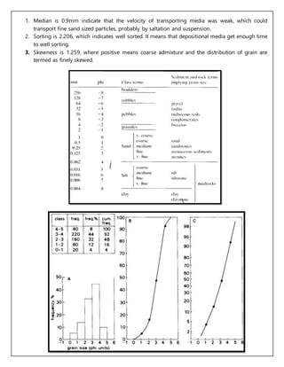
This document reports the results of a grain size analysis of two sandstone samples: 1) Dupitila sandstone - The histogram shows a bimodal distribution with modes between 0.5-1 mm and 0.25-0.125 mm. The median is 0.175 mm. Sorting is well at 2.68 and skewness is finely skewed at 2.21. 2) Surma Group sandstone - The histogram again shows a bimodal distribution with modes above 1 mm and 0.125-0.063 mm. The median is 0.9 mm. Sorting is well at 2.206 and skewness is finely skewed at 1.259.

1. Sample no: 01
Name of the sample: Dupitila sandstone.
Time of sieving: 20min
Amount of sample: 100gm
Diameter in mm Weight retain in gm Weight percent in gm Cumulative weight
percent in gm.
0.50 3.51 3.51 3.51
0.25 39.20 39.20 42.71
0.125 29.13 29.13 71.84
0.063 13.16 13.16 85.00
PAN 14.99 14.99 99.99
Total = 100 gm
Sieve loss= (100 – 99.99) gm
= 0.01
Total coarse sand (wt %) = 36.99
Total coarse sand (wt %) = 1.00
Total fine sand (wt %) = 62.15

2. Figure 4.1: Histogram of Dupitila sandstone
Description of histogram:
By using grain size analytical data the histogram has been drawn. Here an ordinary arithmetic
graph paper is used. Histogram is drawn by taking weight percent retain in the vertical scale verses
grain size in mm in the horizontal scale. The histogram shows a bimodal grain size distribution having
modal class between 1.00 mm to 0.5 mm and 0.25mm to 0.125mm is called primary maxima and
secondary maxima respectively.
Bimodal distribution of grain size may result due to any of the following regions-
 Abnormal variation in depositional energy.
 Lack or abundance of certain grain size in the source materials.
 Mixing of materials from two or more sources.
 Different modes of deposition.
 Improper sampling.
0
5
10
15
20
25
30
35
40
45
0.5 0.25 0.125 0.063 PAN
WeightpercentRetained
Grain Size in phi Scale
Histogram of Dupitila Sandstone

3. Figure 4.2: Cumulative curve of Dupitila sandstone
Cumulative curve:
By taking cumulative weight percent in vertical scale and grain size in mm in the horizontal
scale the cumulative curve has been drawn. The figure gives an “S” shaped curve from which quartile
and percentile have been determined in order to calculate the grain size parameter according to Trask
Method.
25 percentile (25p) or 1st
quartile (Q1) = 0.72 mm.
50 percentile (50p) or 2nd
quartile (Q2) = 0.177mm.
75 percentile (75p) or 3rd
quartile (Q3) = 0.096875mm.
Median (Md) = 50p = 0.175mm.
Co-efficient of sorting, So = Q1/Q3 = 0.72/0.096875 = 2.68
Co-efficient of skewness, Sk = Q1Q3/Md2
= (0.7x 0.096875)/(0.177)2=
2.21
From Trask Method,
0
20
40
60
80
100
120
>.50 0.25 0.125 0.063 <.063
Cumulative Weigth Percentage (gm)
Cumulative Weigth Percentage
(gm)

4. 1. Median (Md) is 0.175 indicates that the velocity of the transporting media was weak which
could transport fine sand sized particles probably by saltation and suspension.
2. Sorting (So) is 2.68 indicates well sorted. It means that, depositional media get enough time to
well sorted.
3. Skewness (Sk) is 2.21 which means that the coarse admixture exceeds the finer admixture and
the distribution of the grains are termed as finely skewed.
Sample no: 02
Name of the sample: Surma Group.
Time of sieving: 20min
Amount of sample: 100gm
Diameter in
mm Weight retain in gm
Weight percent in
gm
Cumulative weight
percent in gm
0.50 5.51 5.51 5.51
0.25 37.20 37.20 42.71
0.125 37.13 27.13 69.84
0.063 13.15 13.15 82.99
PAN 16.99 16.99 99.98
Total = 100 gm
Sieve loss= (100 – 99.98) gm
= 0.02 gm.
Total coarse sand (wt %) = 80.38
Total medium sand (wt %) = 0.25
Total fine sand (wt %) = 18.745

5. Figure 4.3: Histogram of Tipam sandstone
Description of histogram:
By using grain size analytical data the histogram has been drawn. Here an ordinary arithmetic
graph paper is used. Histogram is drawn by taking weight percent retain in the vertical scale verses
grain size in mm in the horizontal scale. The histogram shows a bimodal grain size distribution having
modal class between >1.00 mm and 0.125mm to 0.0625mm is called primary maxima and secondary
maxima respectively.
Bimodal distribution of grain size may result due to any of the following regions-
 Abnormal variation in depositional energy.
 Lack or abundance of certain grain size in the source materials.
 Mixing of materials from two or more sources.
 Different modes of deposition.
 Improper sampling.
0
5
10
15
20
25
30
35
40
0.5 0.25 0.125 0.063 PAN
WeightPercentRetained
Grain Size in phi Scale
Histogram of Surma Sandstone

6. Figure 4.4: Cumulative curve of Tipam sandstone
Cumulative curve:
By taking cumulative weight percent in vertical scale and grain size in mm in the horizontal
scale the cumulative curve has been drawn. The figure gives an “S” shaped curve from which quartile
and percentile have been determined in order to calculate the grain size parameter according to Trask
Method.
25 percentile (25p) or 1st
quartile (Q1) = 1.5mm
50 percentile (50p) or 2nd
quartile (Q2) = 0.9mm.
75 percentile (75p) or 3rd
quartile (Q3) = 0.68mm.
Median (Md) = 50p = 0.9mm.
Co-efficient of sorting, So = Q1/Q3= 1.5/0.68 = 2.206
Co-efficient of skewness, Sk = Q1Q3/Md2
= (1.5x 0.68)/ (0.9)2 =
1.259
From Trask Method,
0
20
40
60
80
100
120
>.50 0.25 0.125 0.063 <.063
Cumulative Weigth Percentage (gm)
Cumulative Weigth
Percentage (gm)

7. 1. Median is 0.9mm indicate that the velocity of transporting media was weak, which could
transport fine sand sized particles, probably by saltation and suspension.
2. Sorting is 2.206, which indicates well sorted. It means that depositional media get enough time
to well sorting.
3. Skewness is 1.259, where positive means coarse admixture and the distribution of grain are
termed as finely skewed.