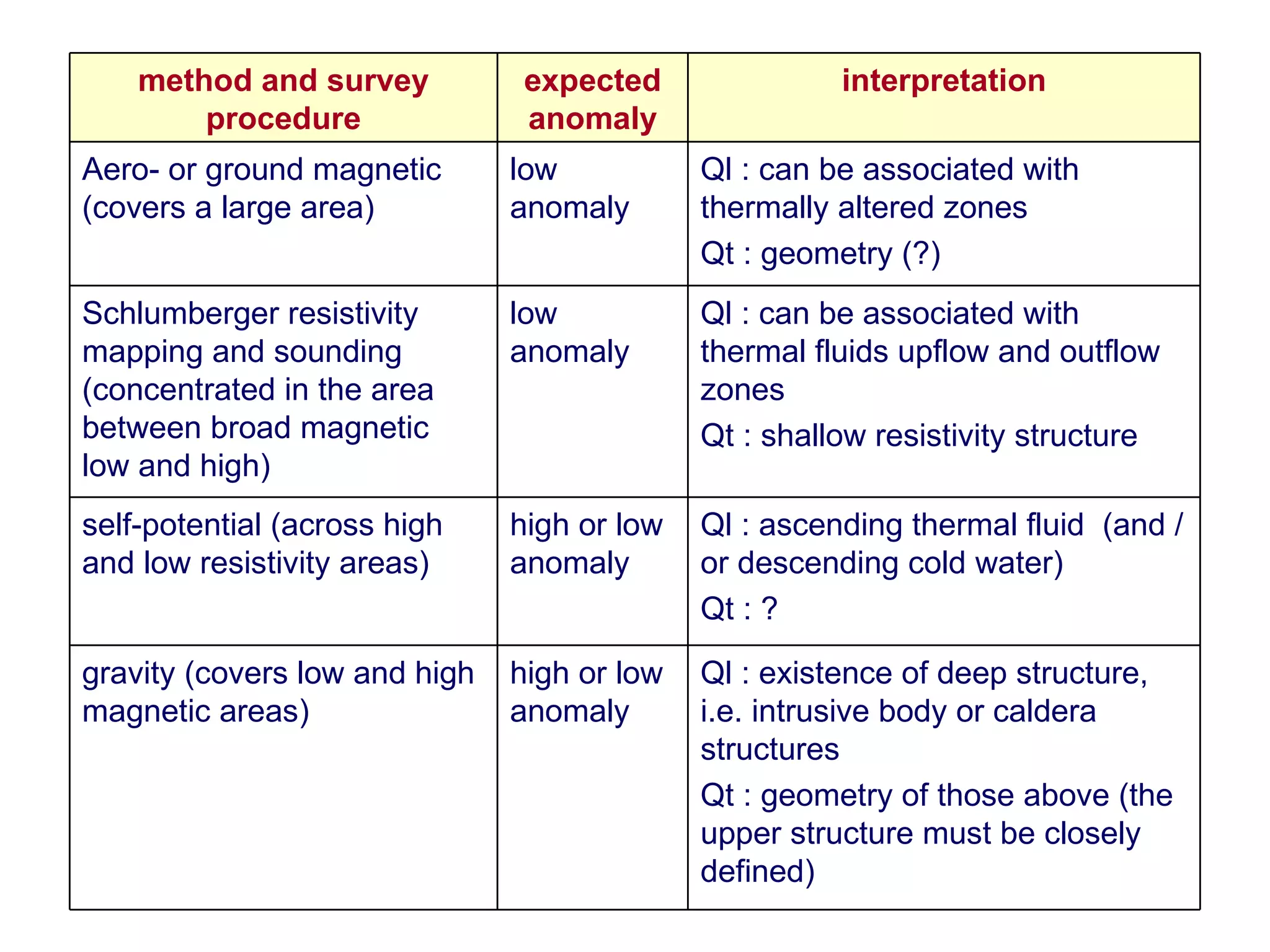
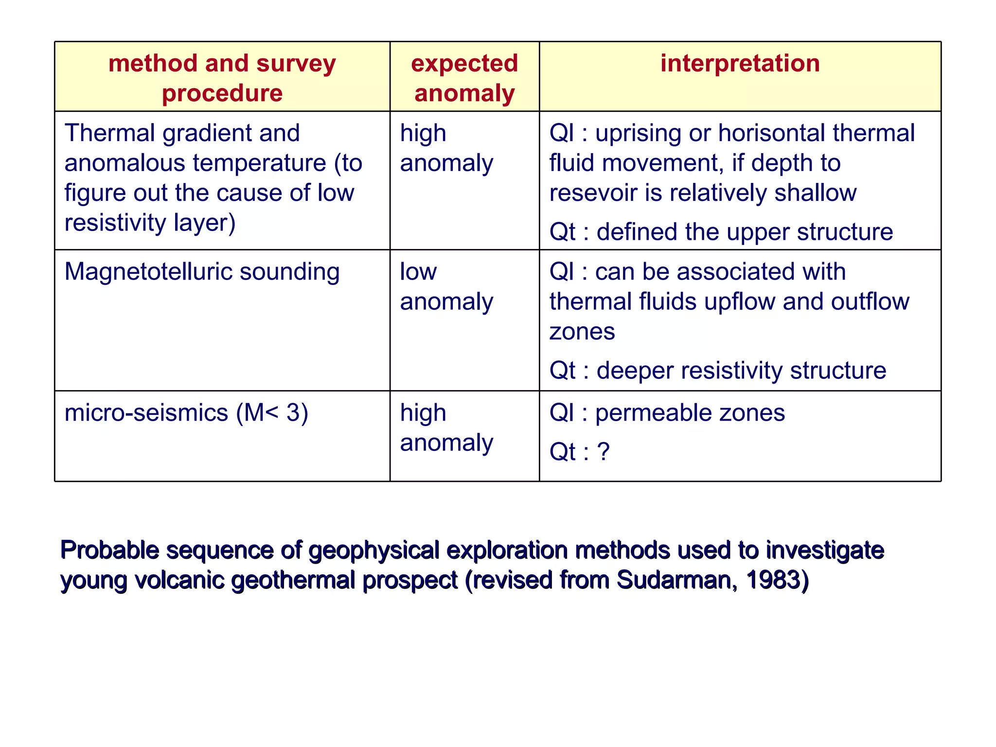
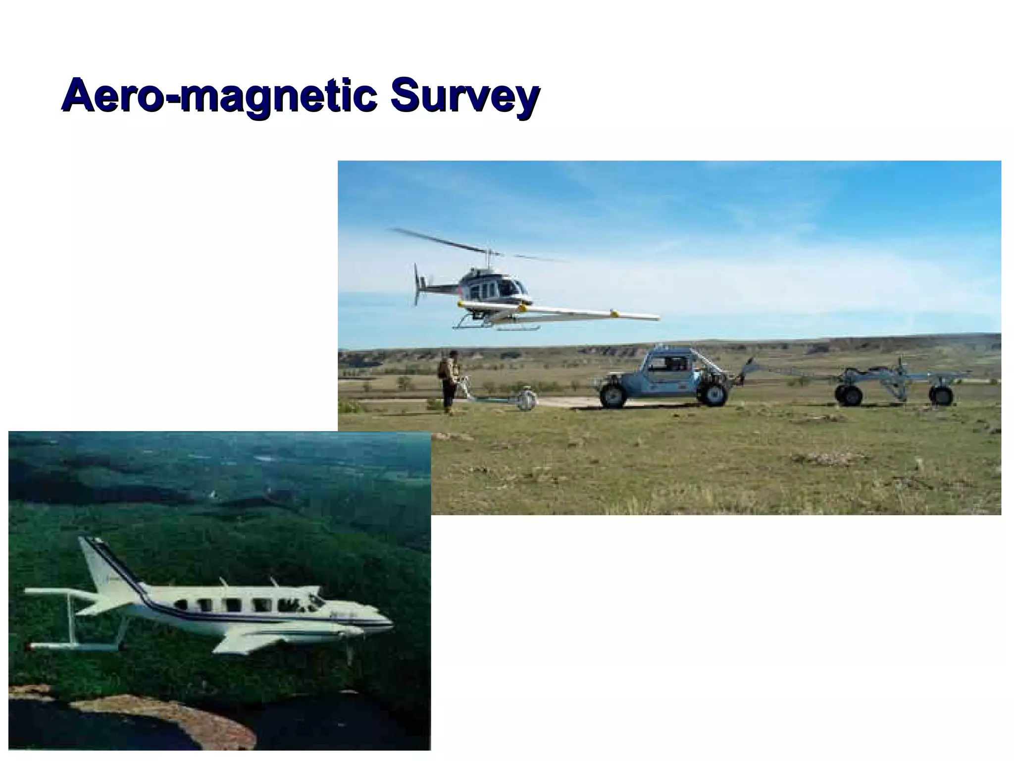
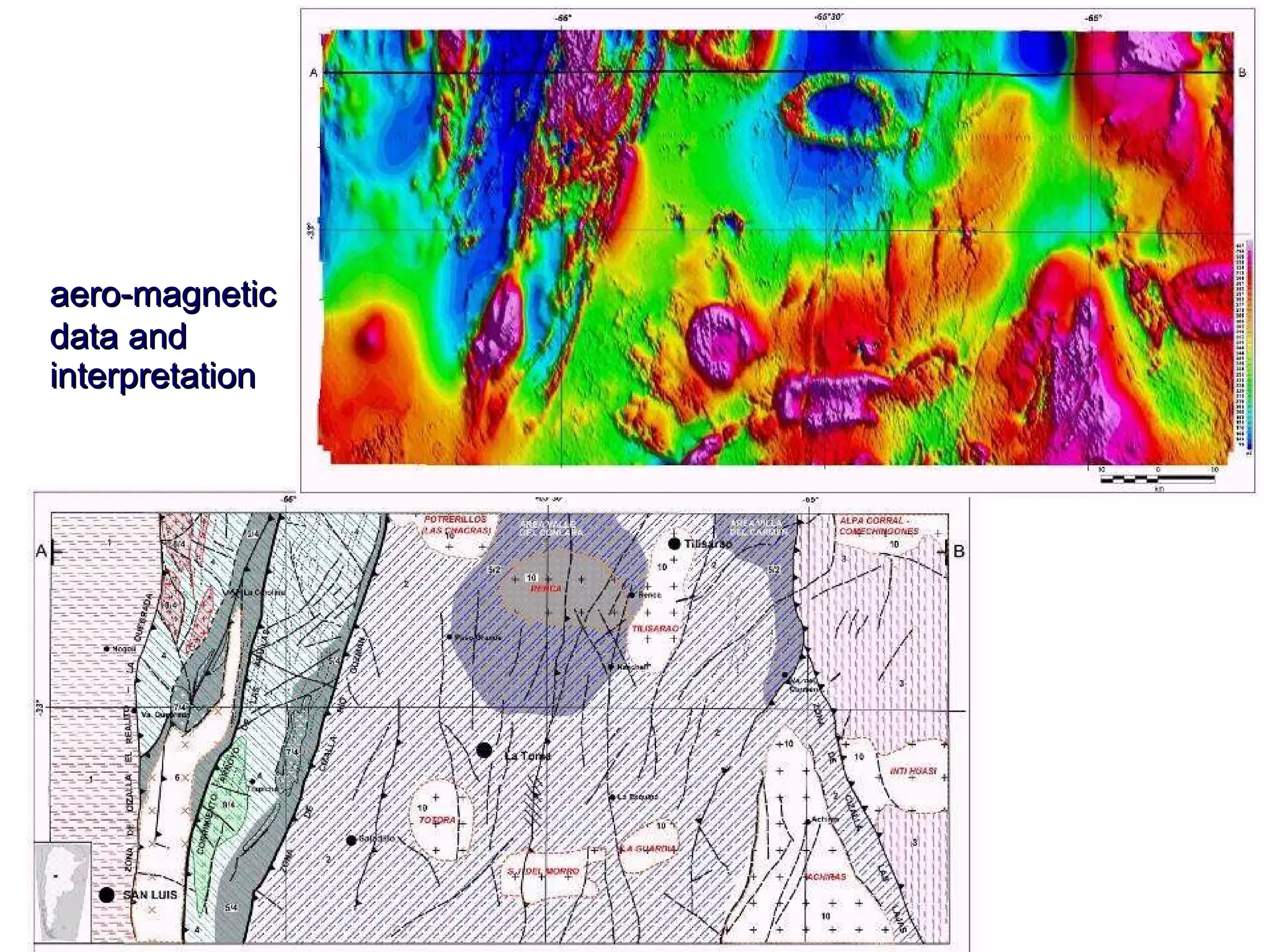
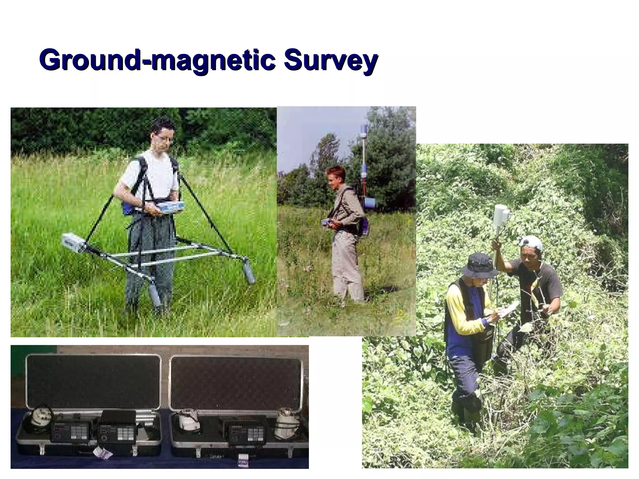
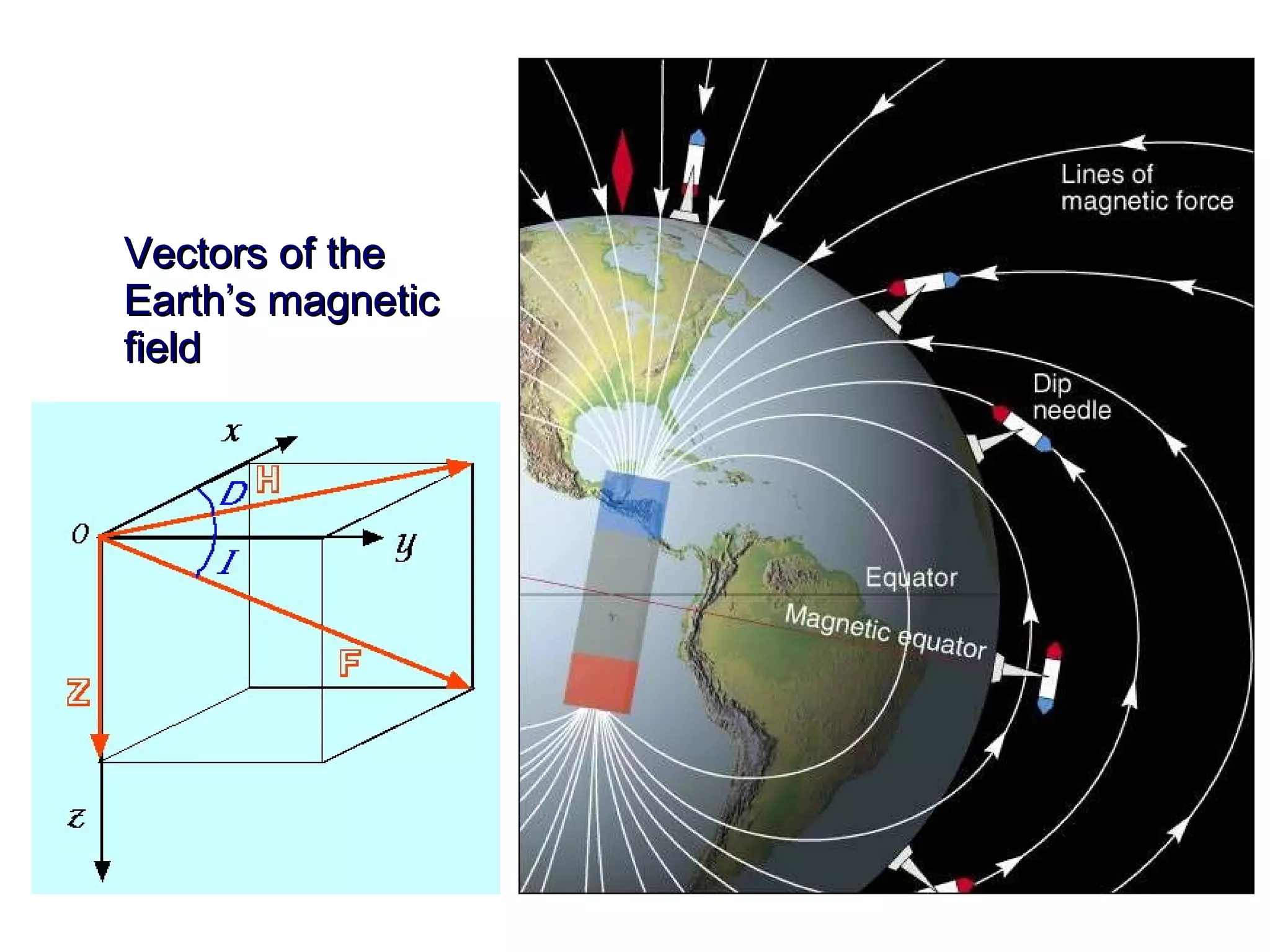
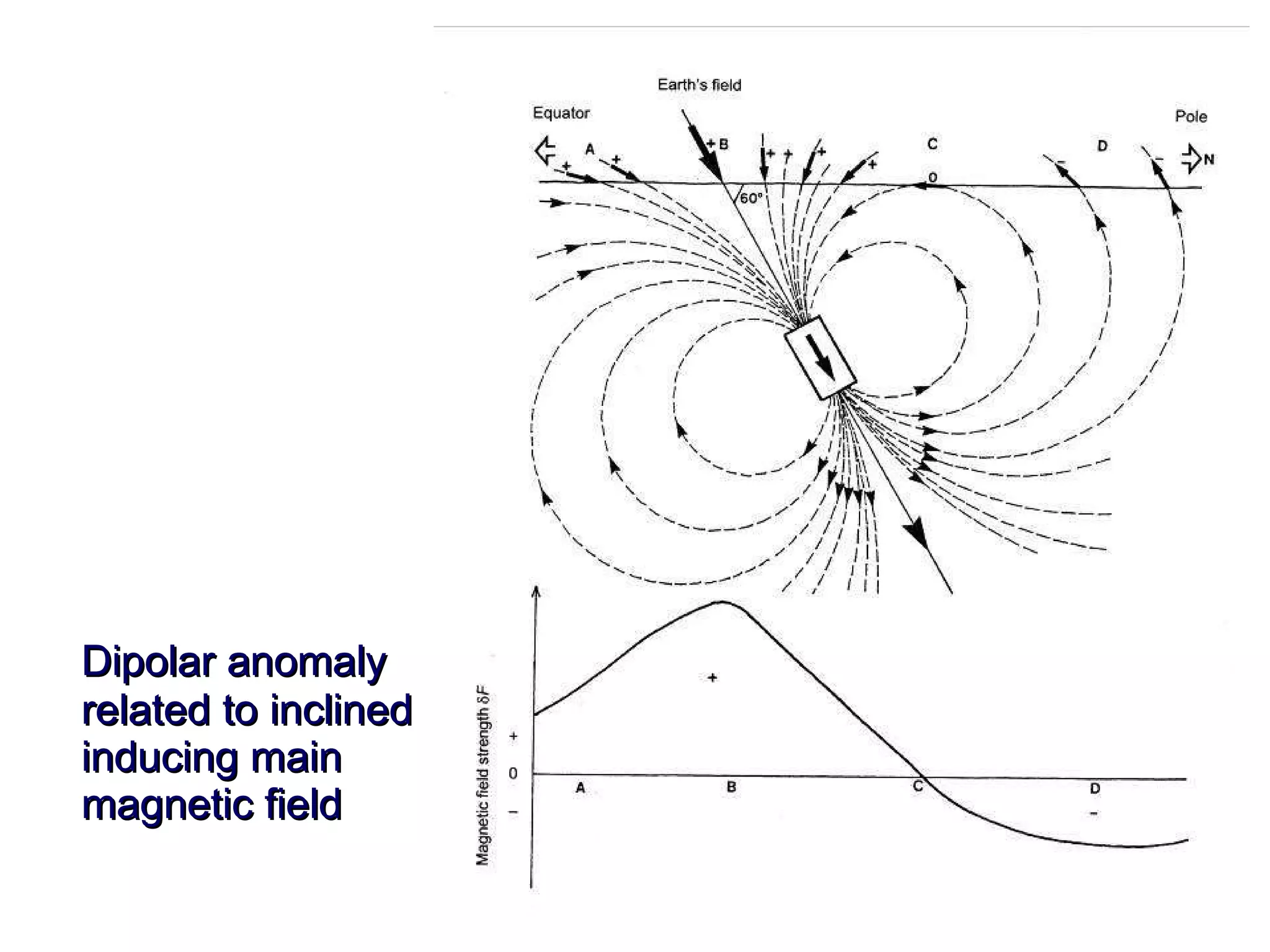
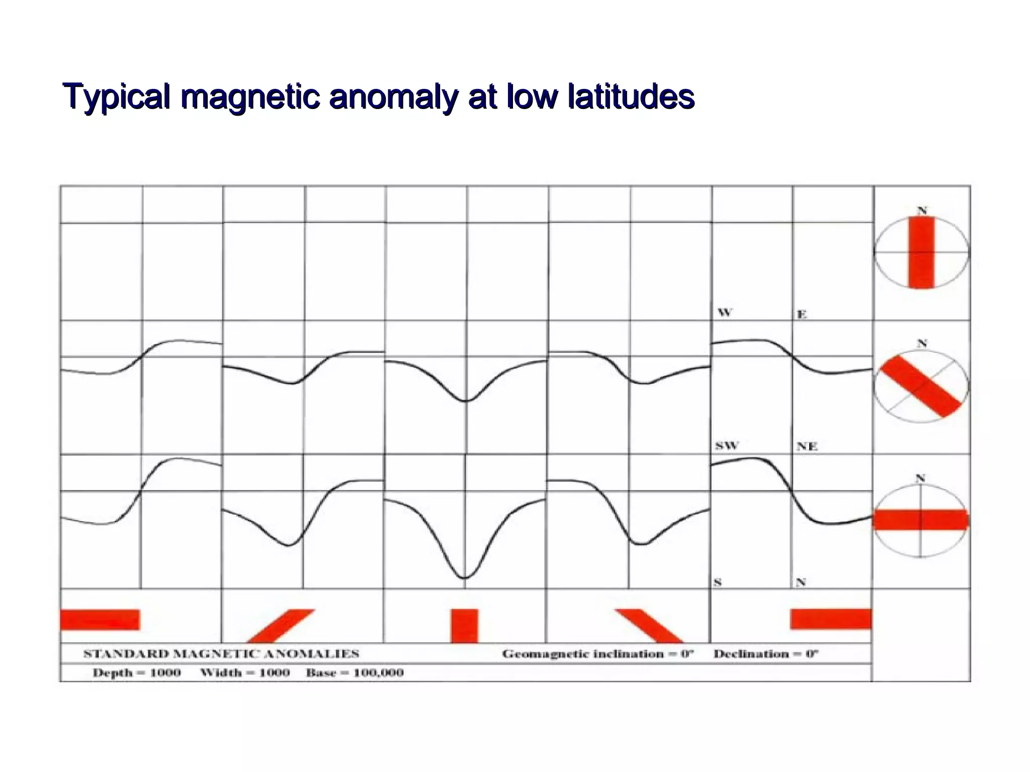
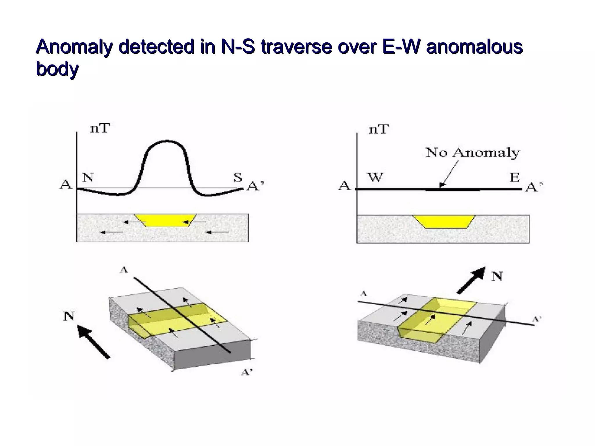
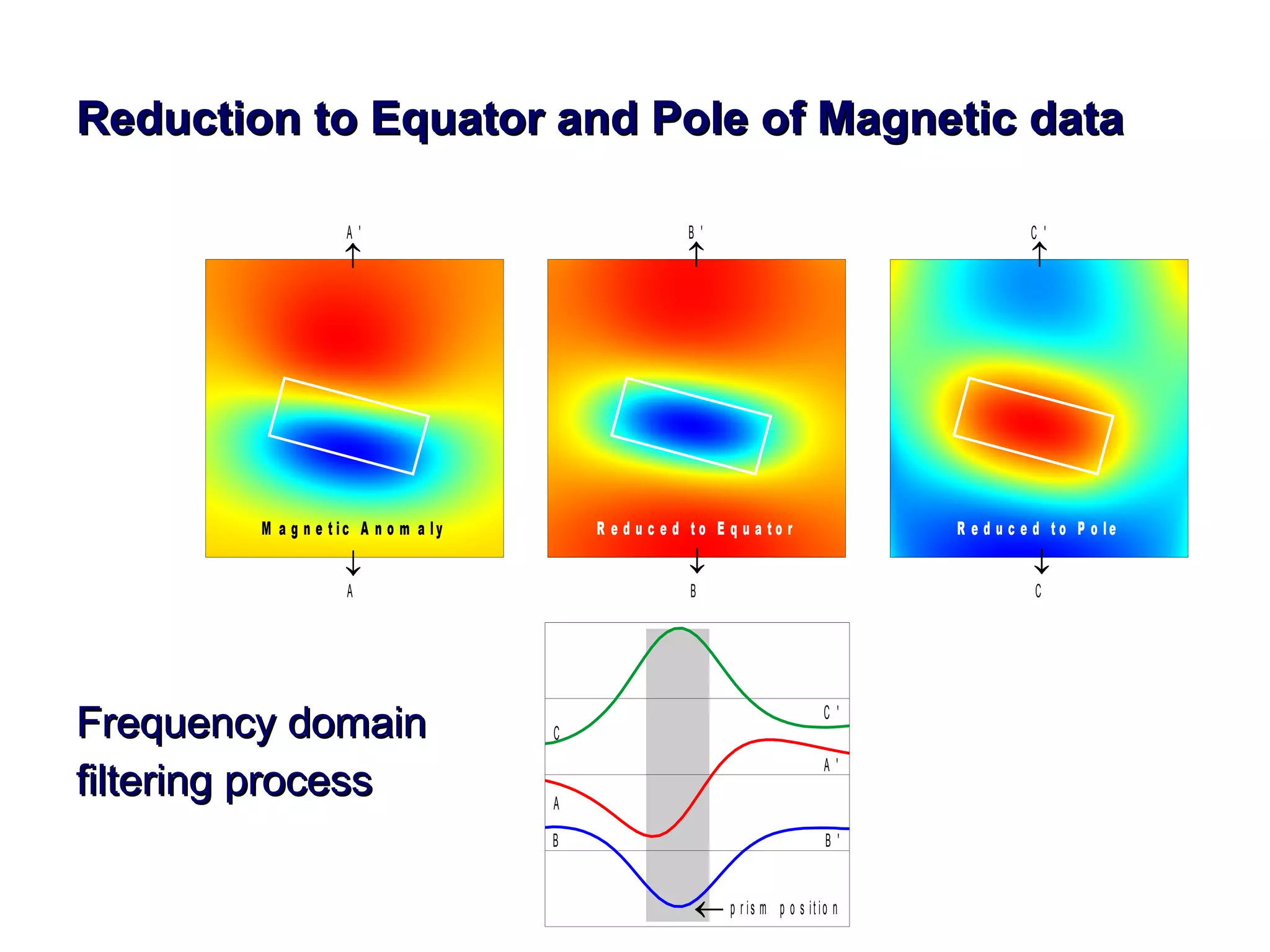
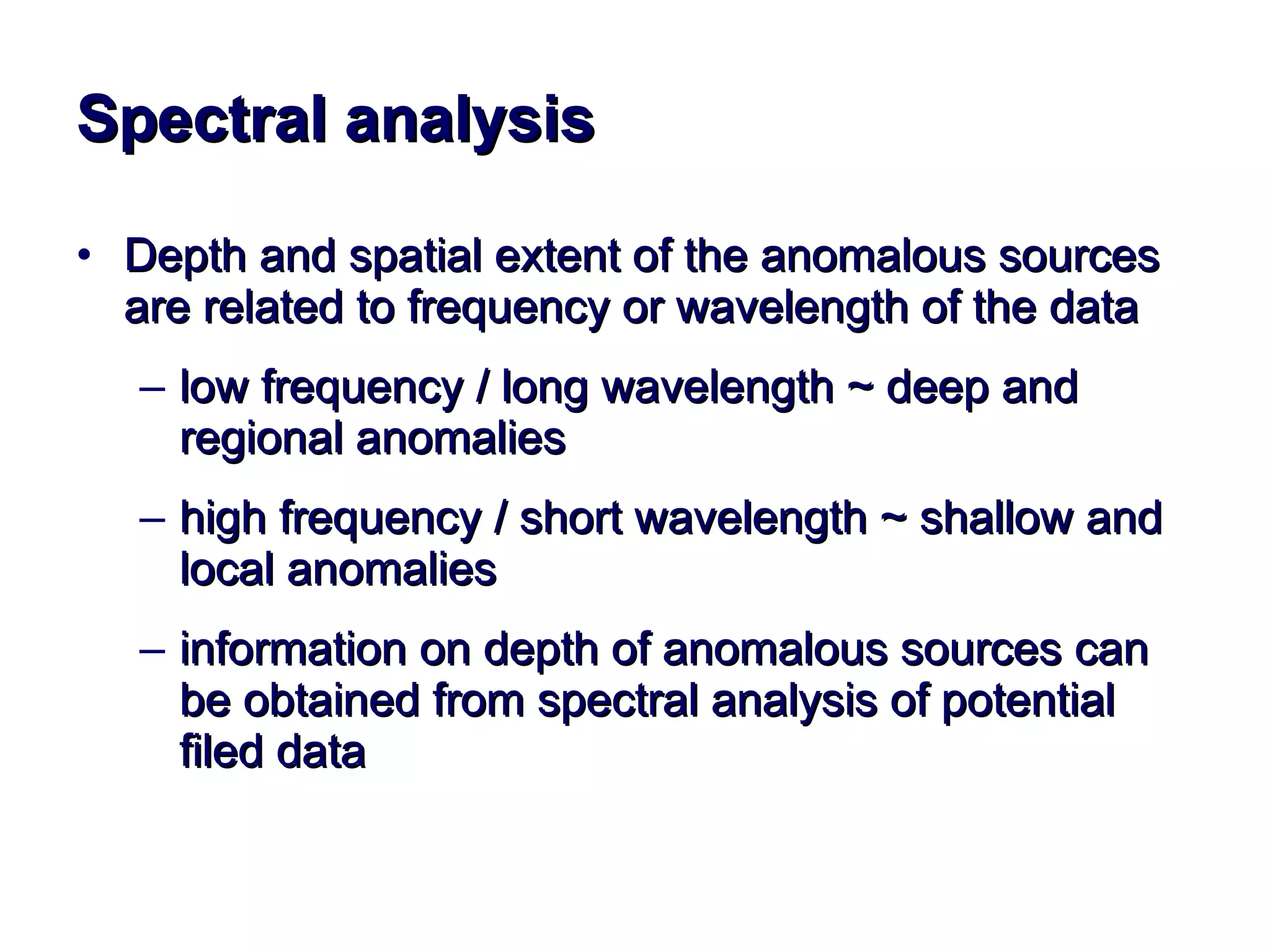
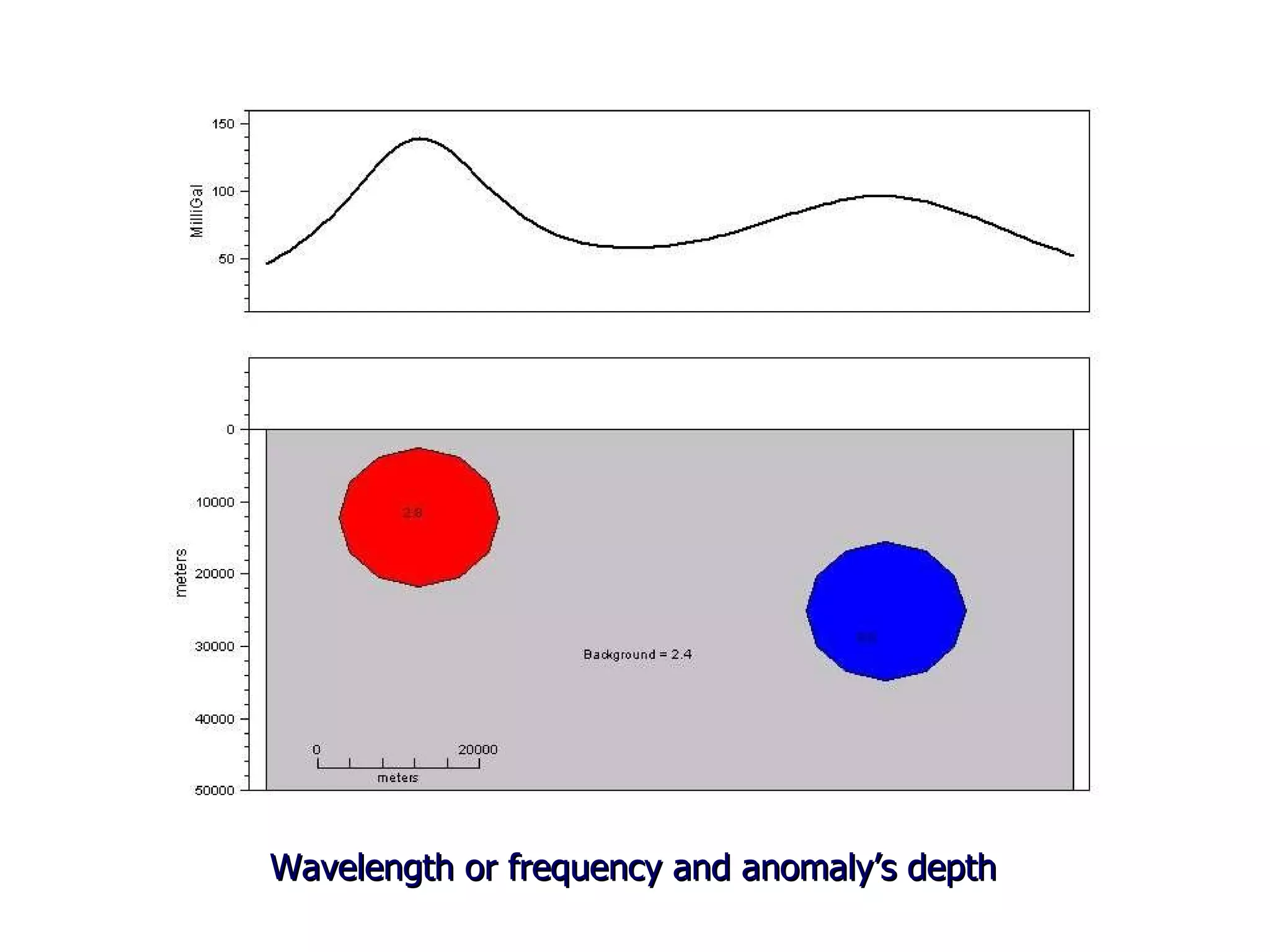
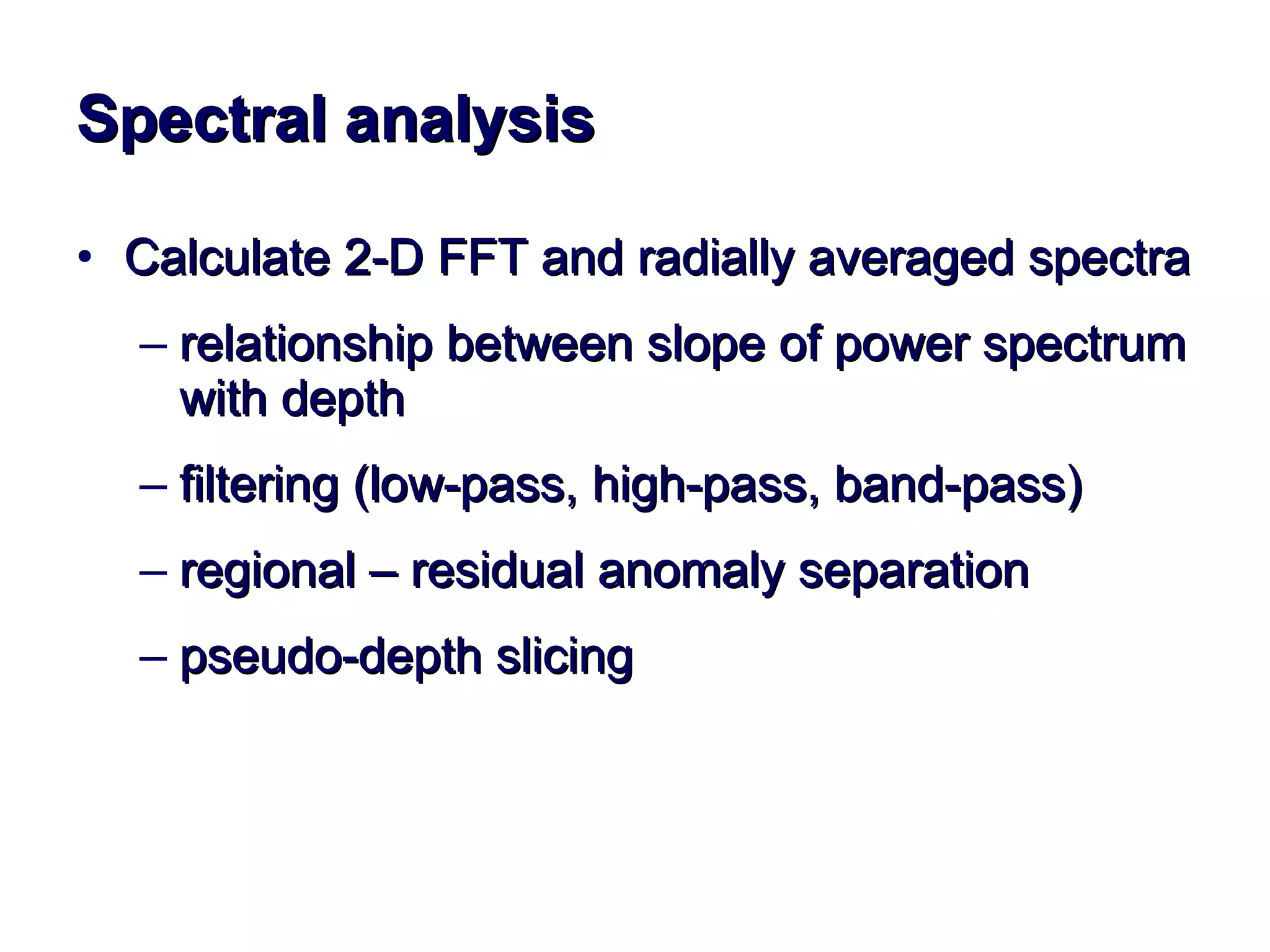
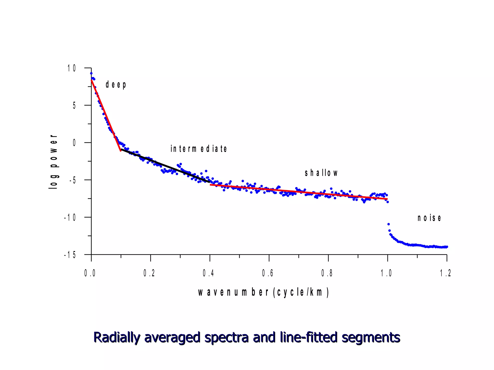
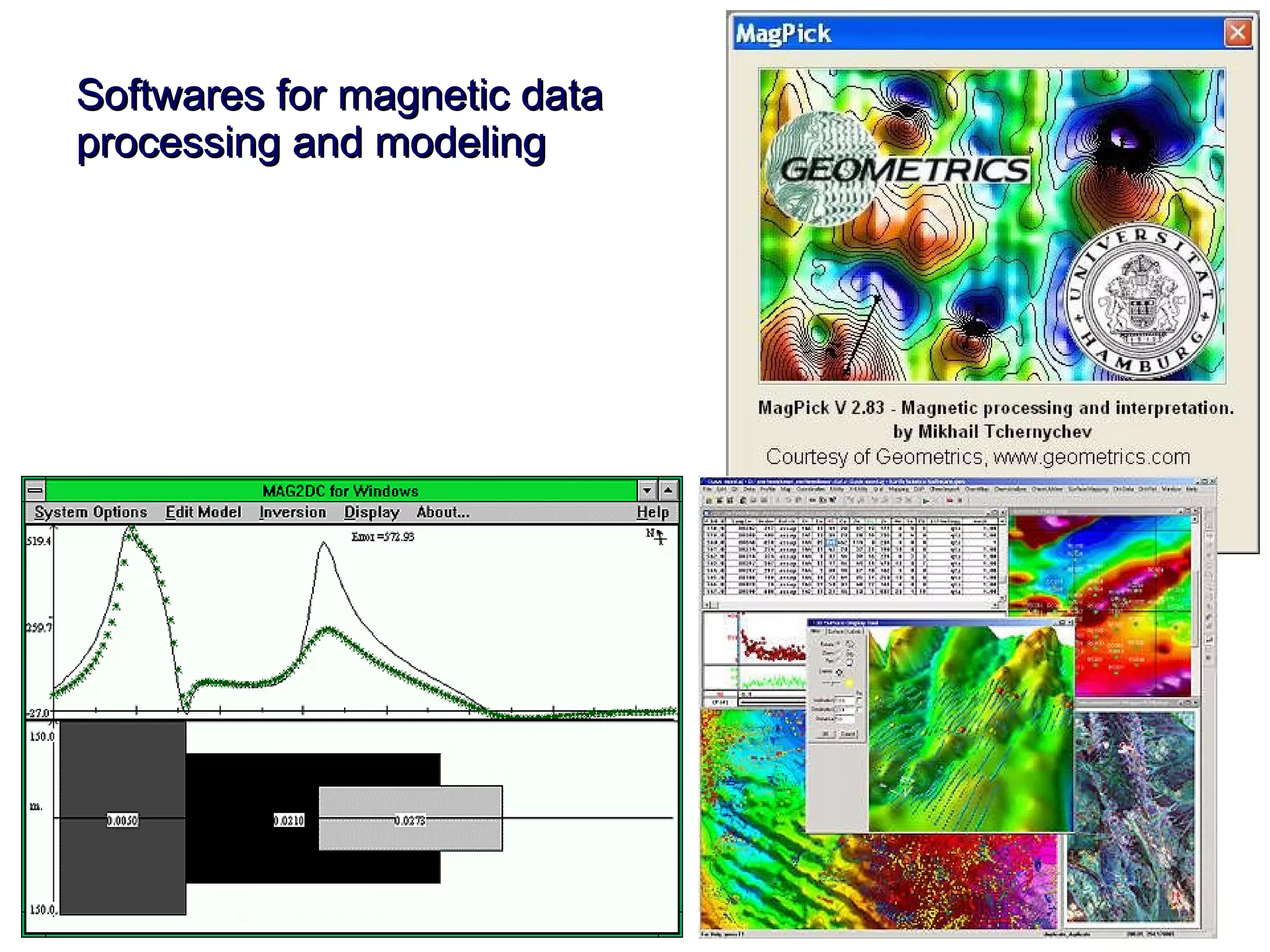
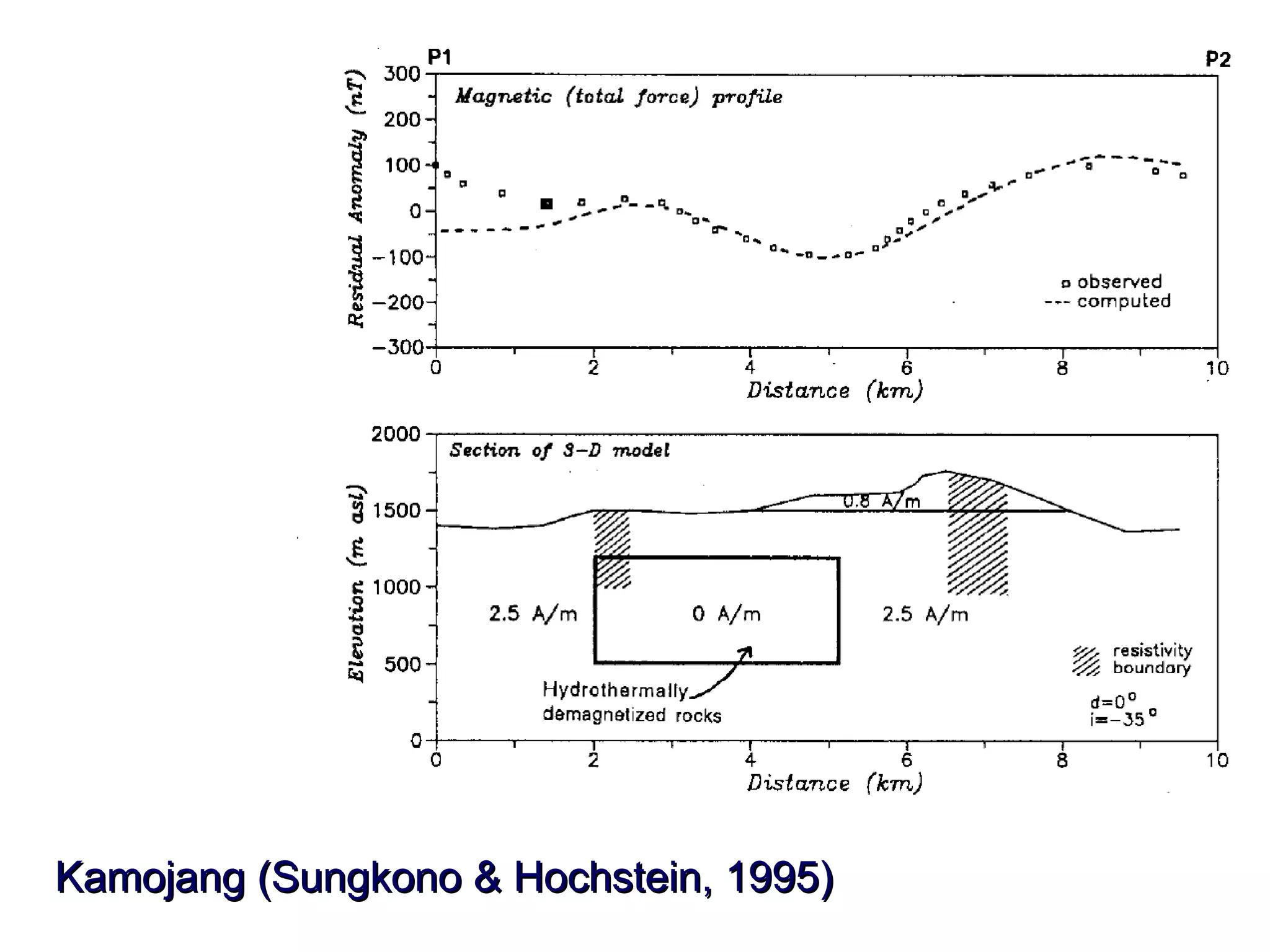
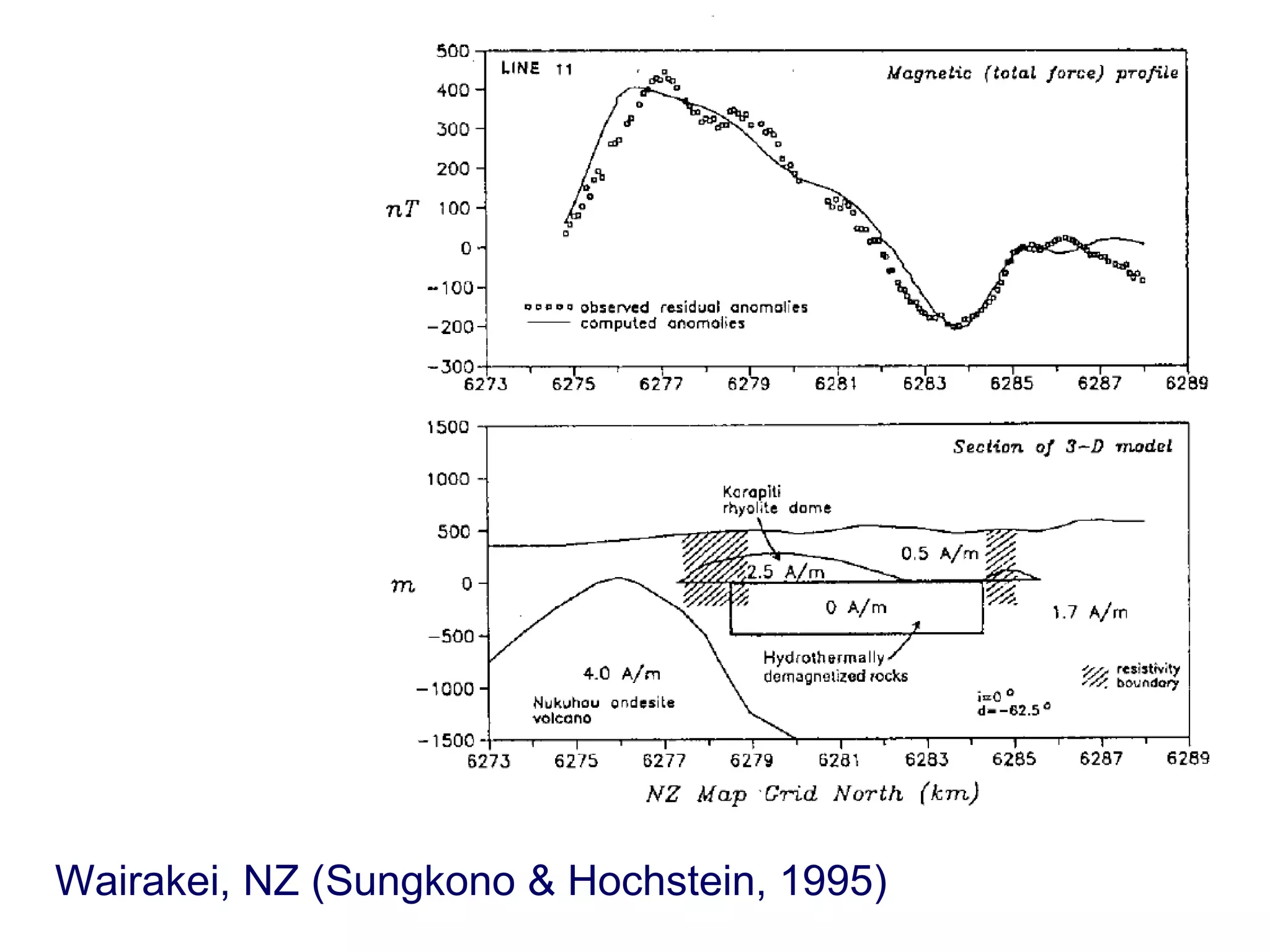
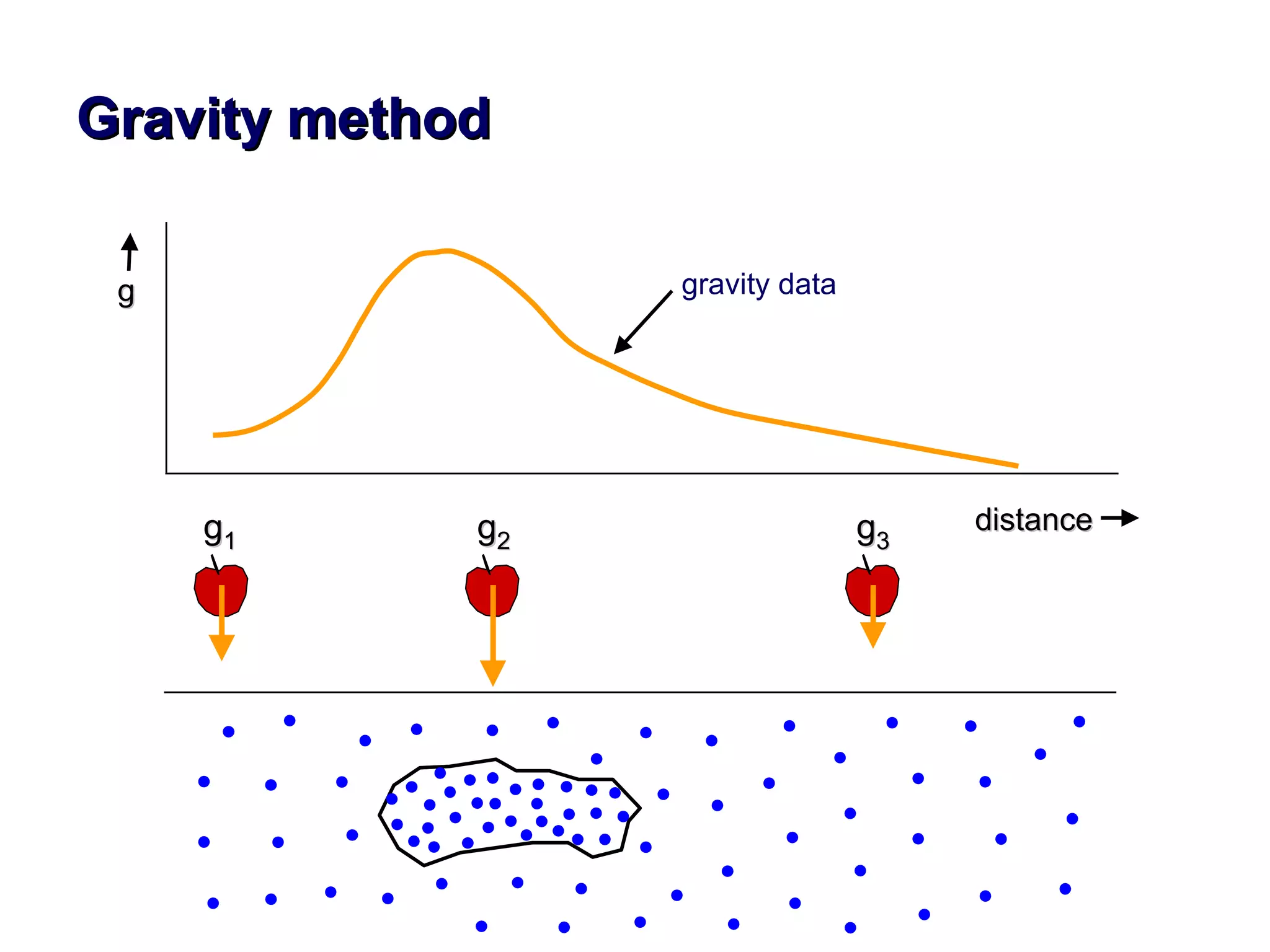
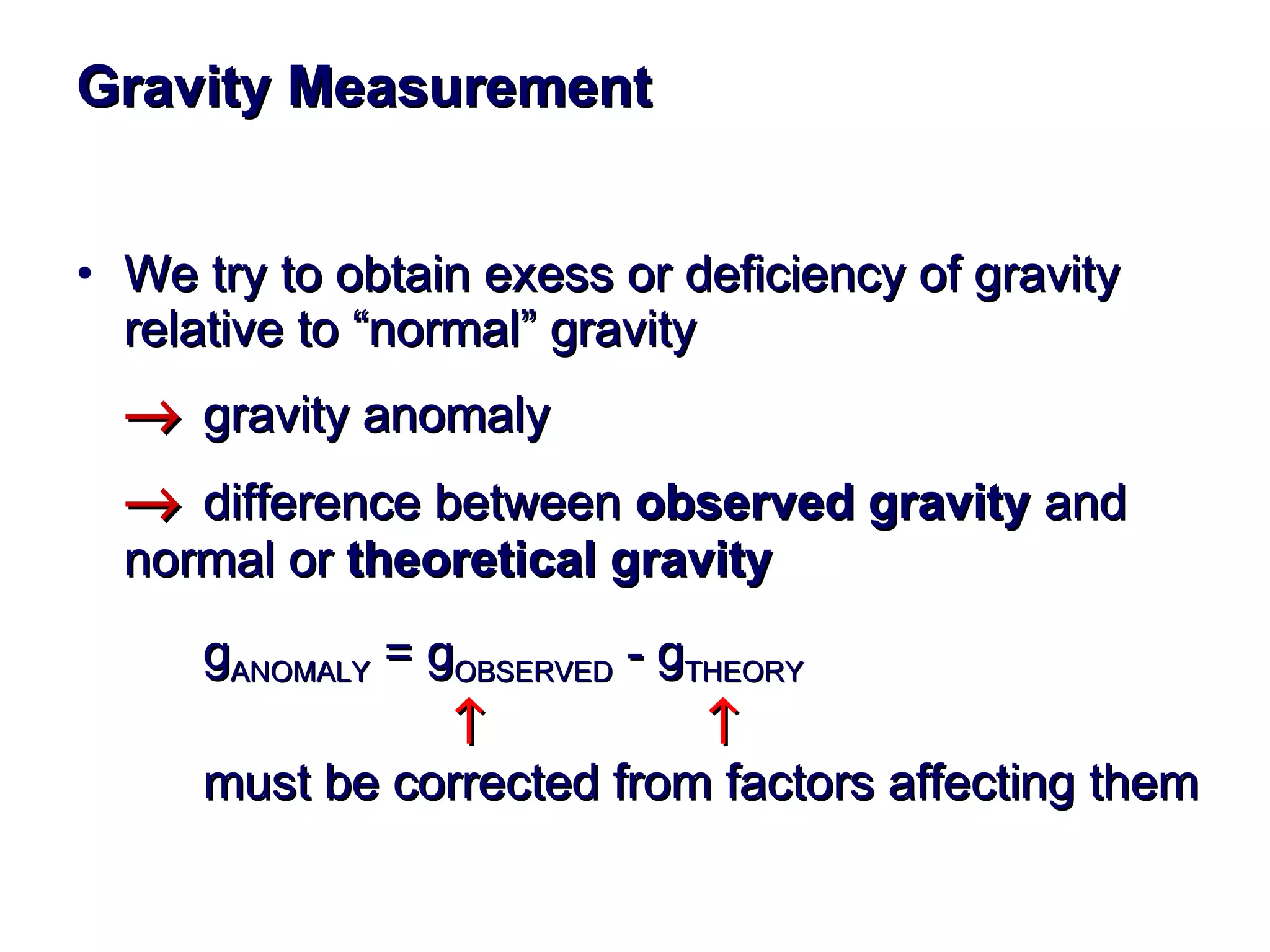
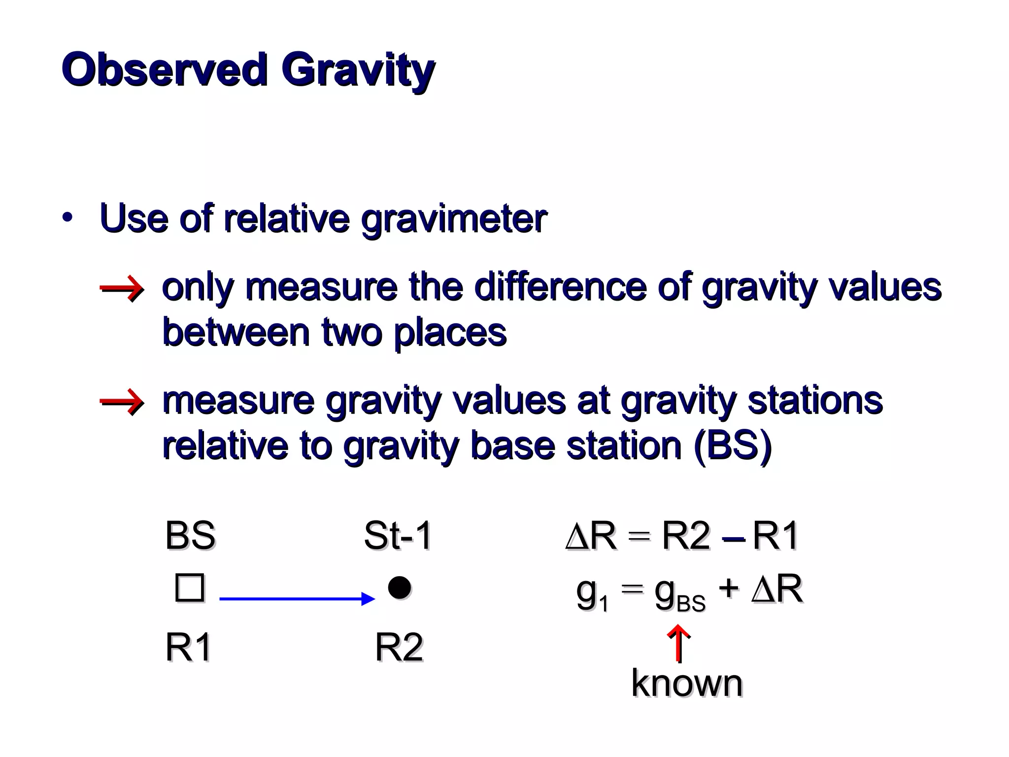
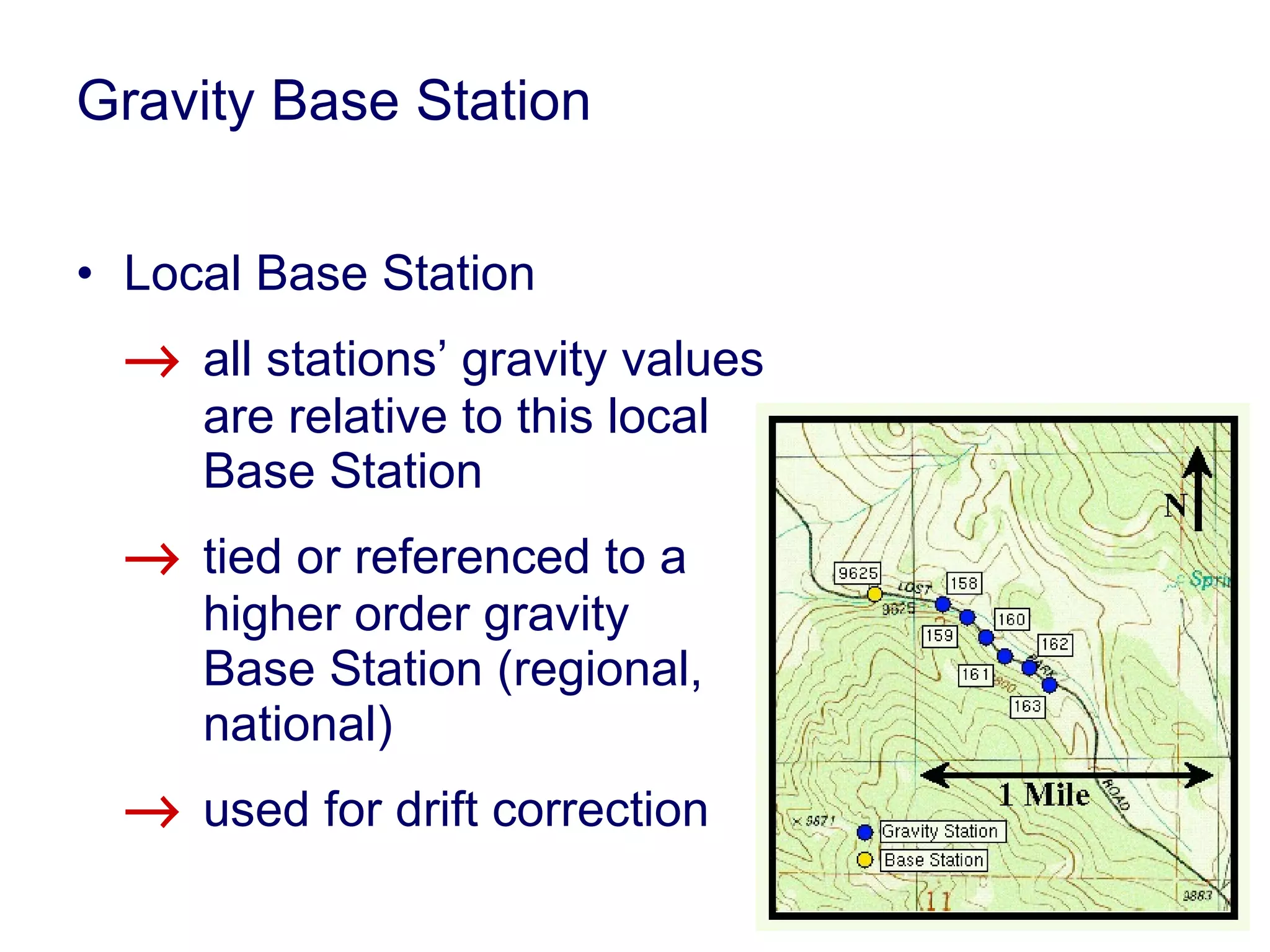
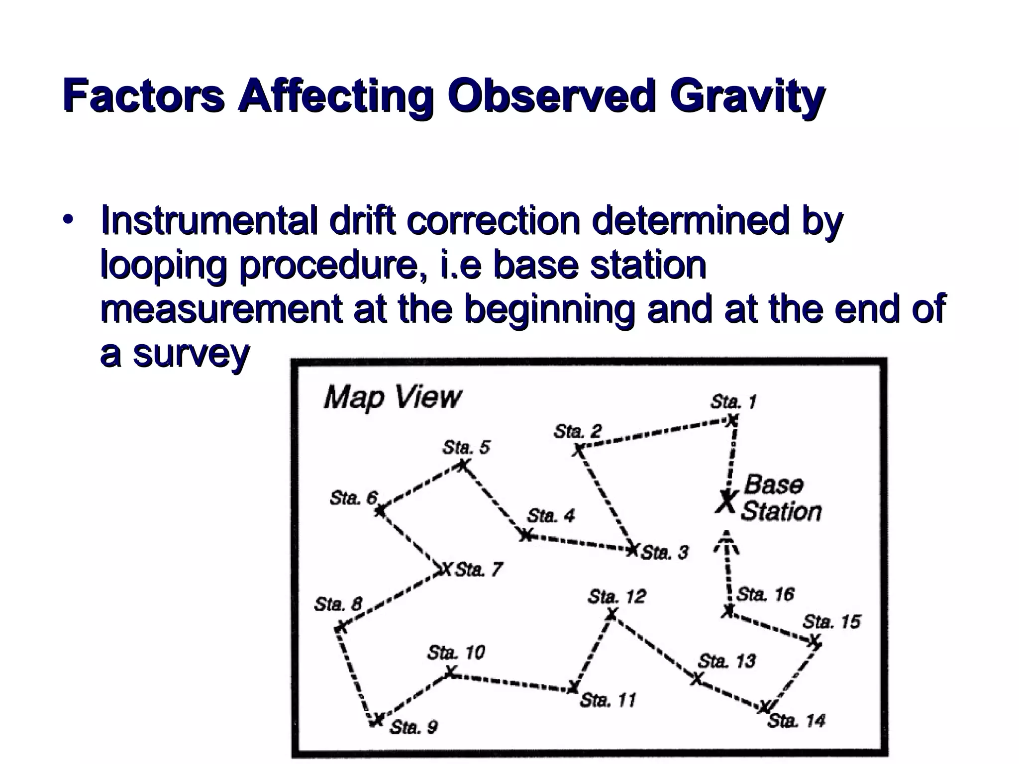
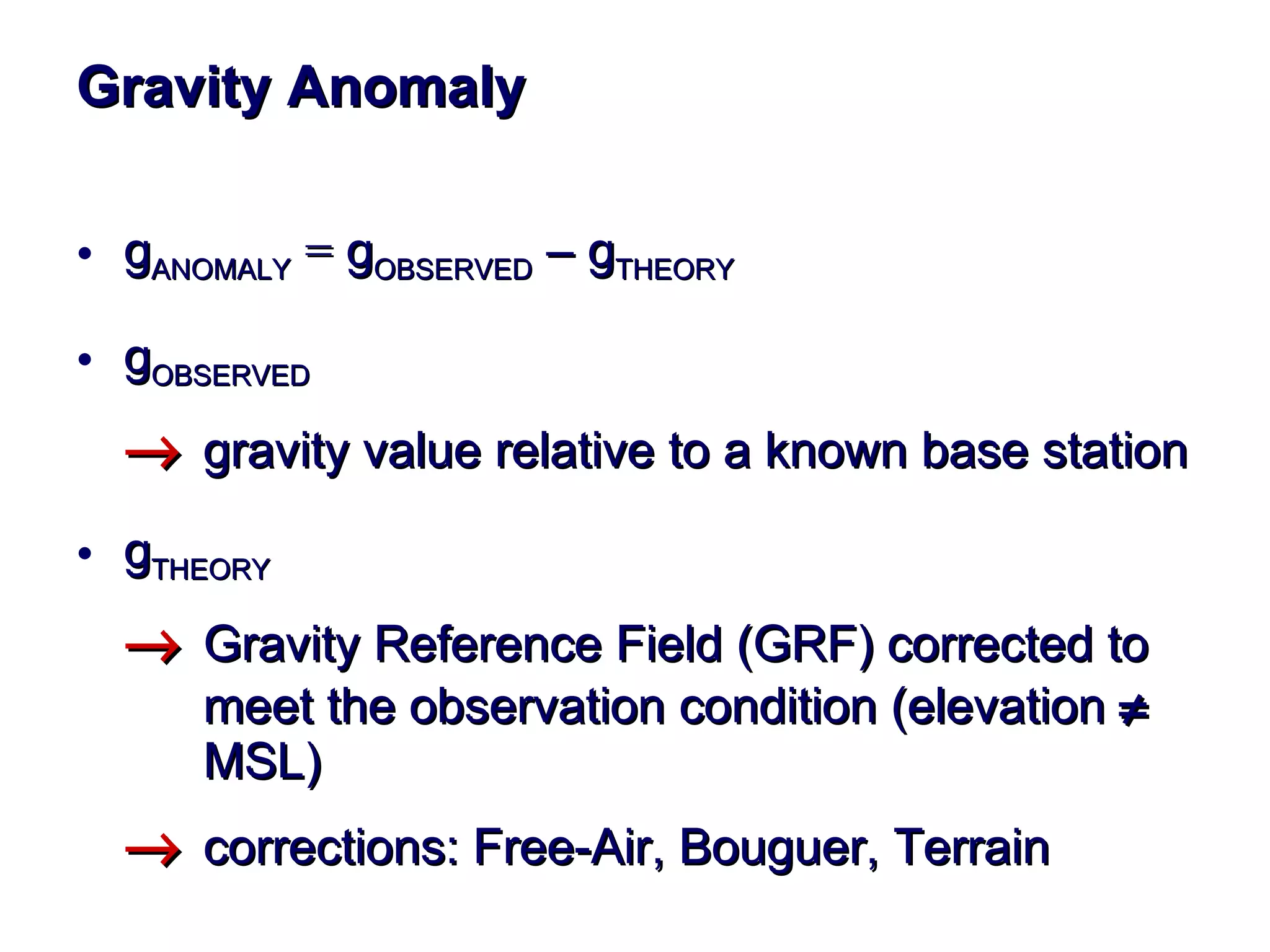
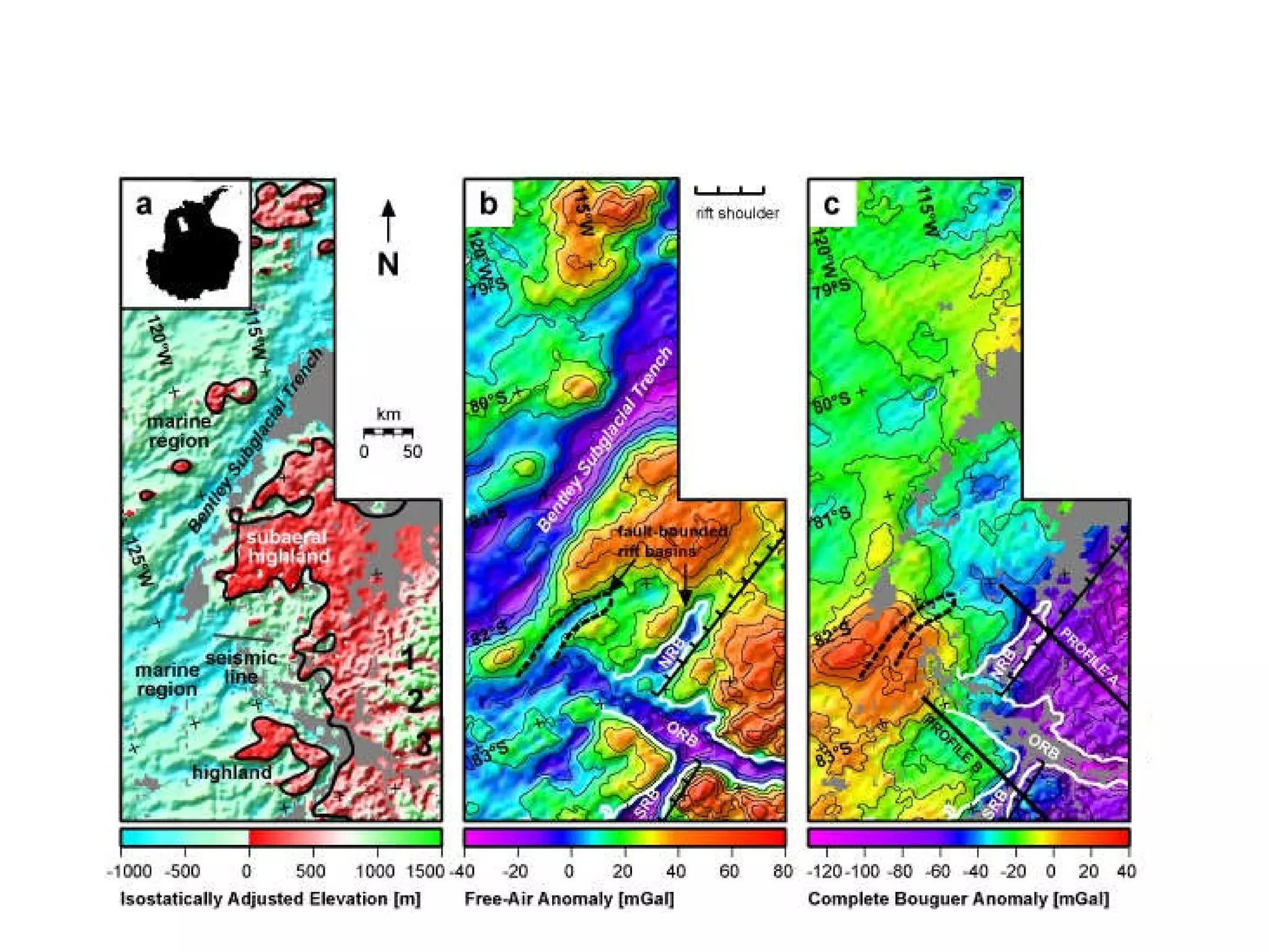
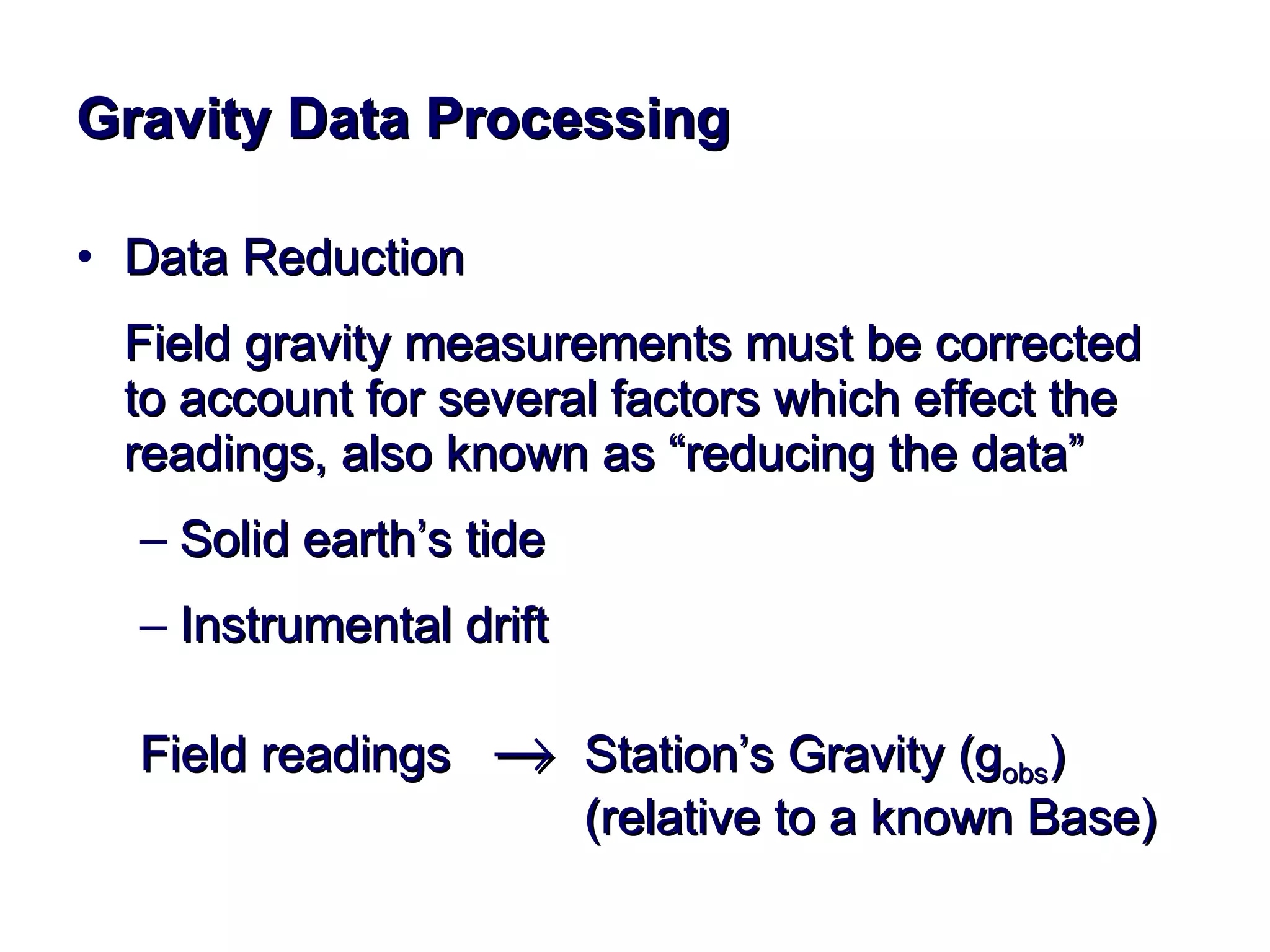
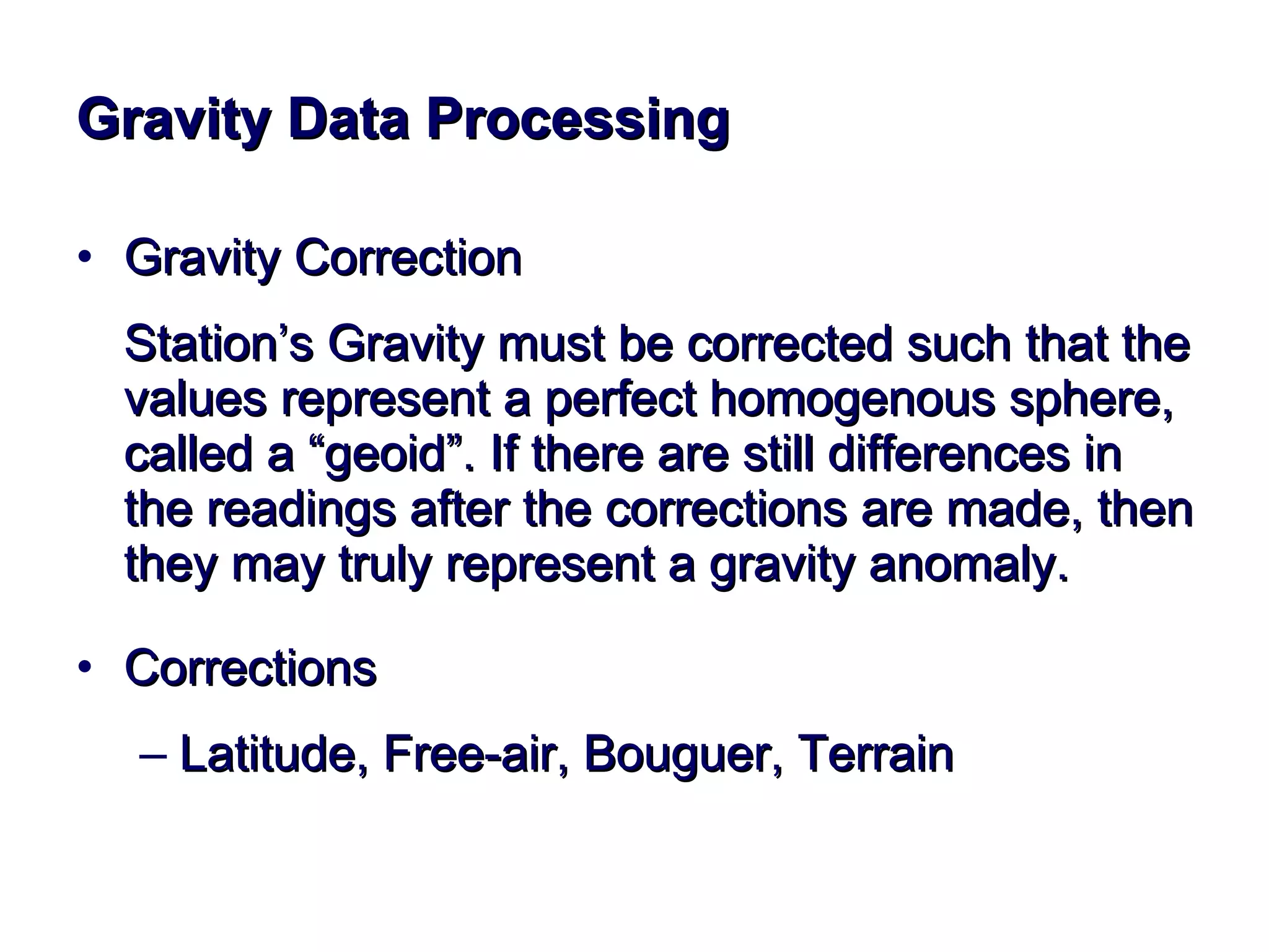
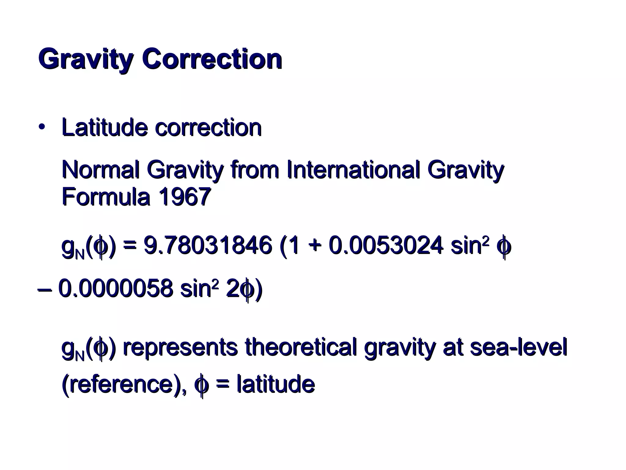
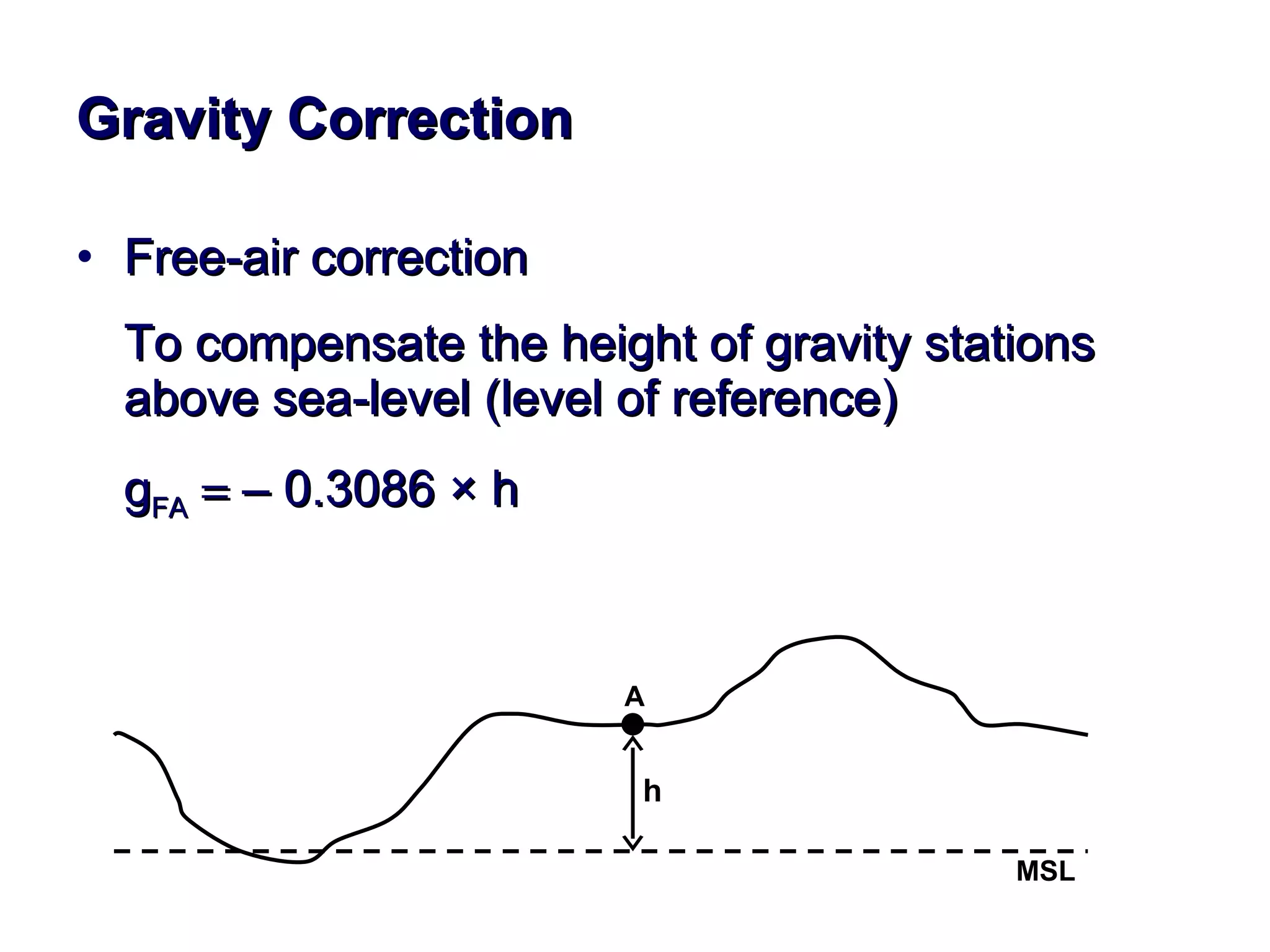
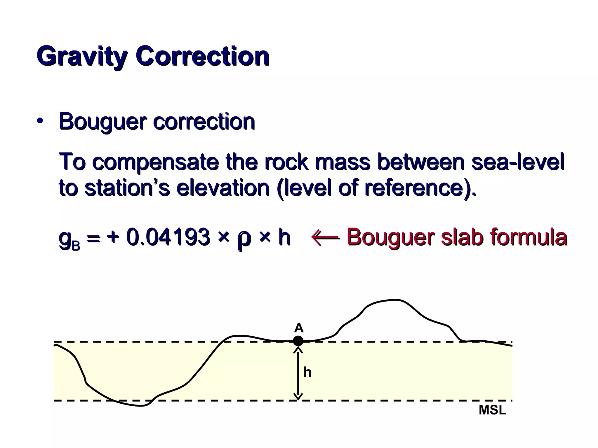
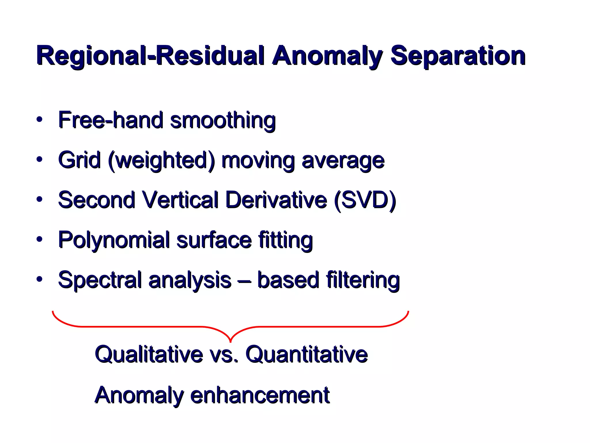
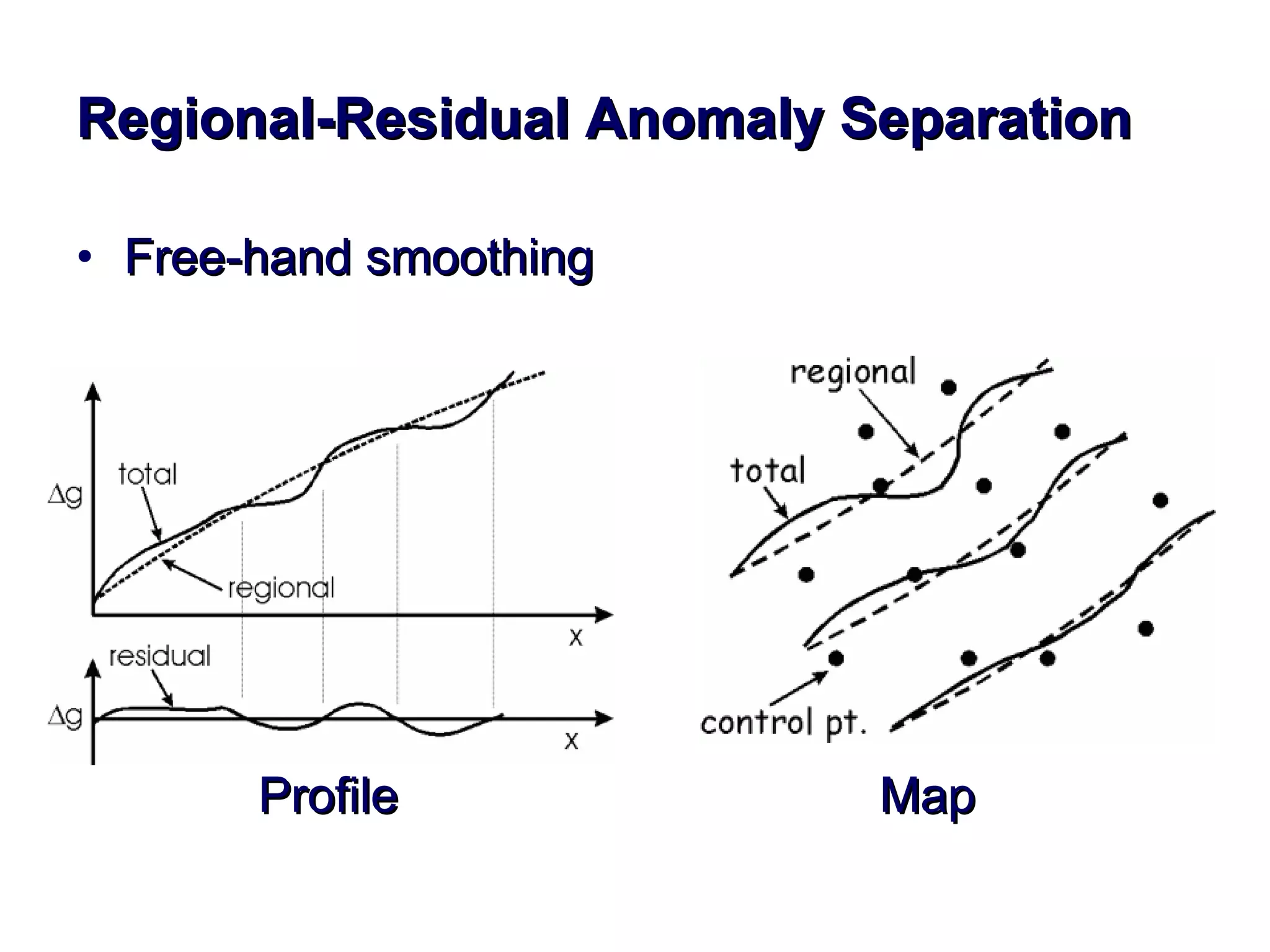
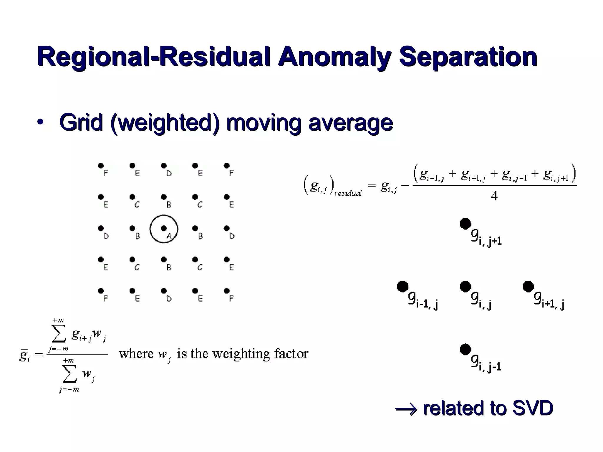
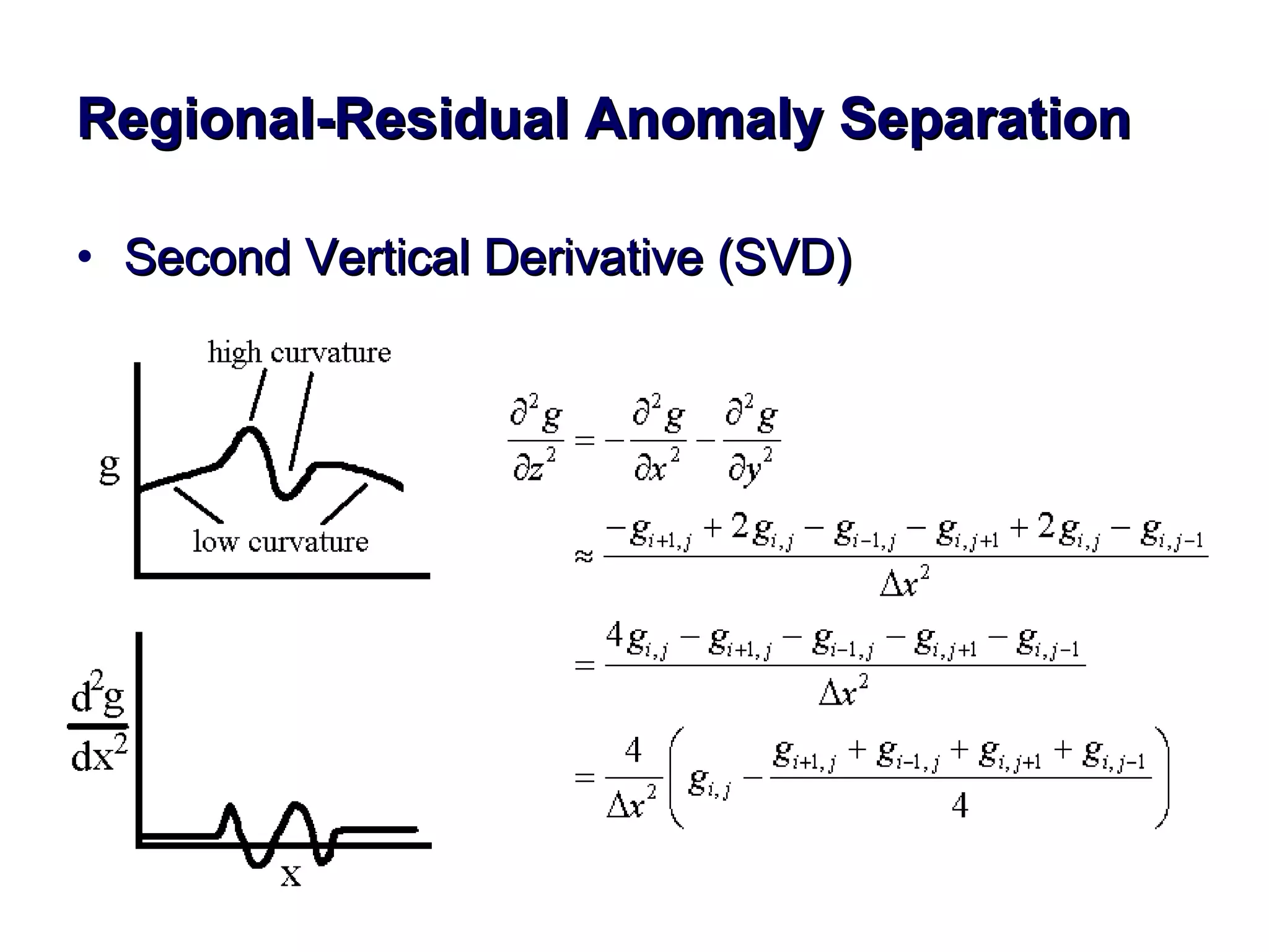
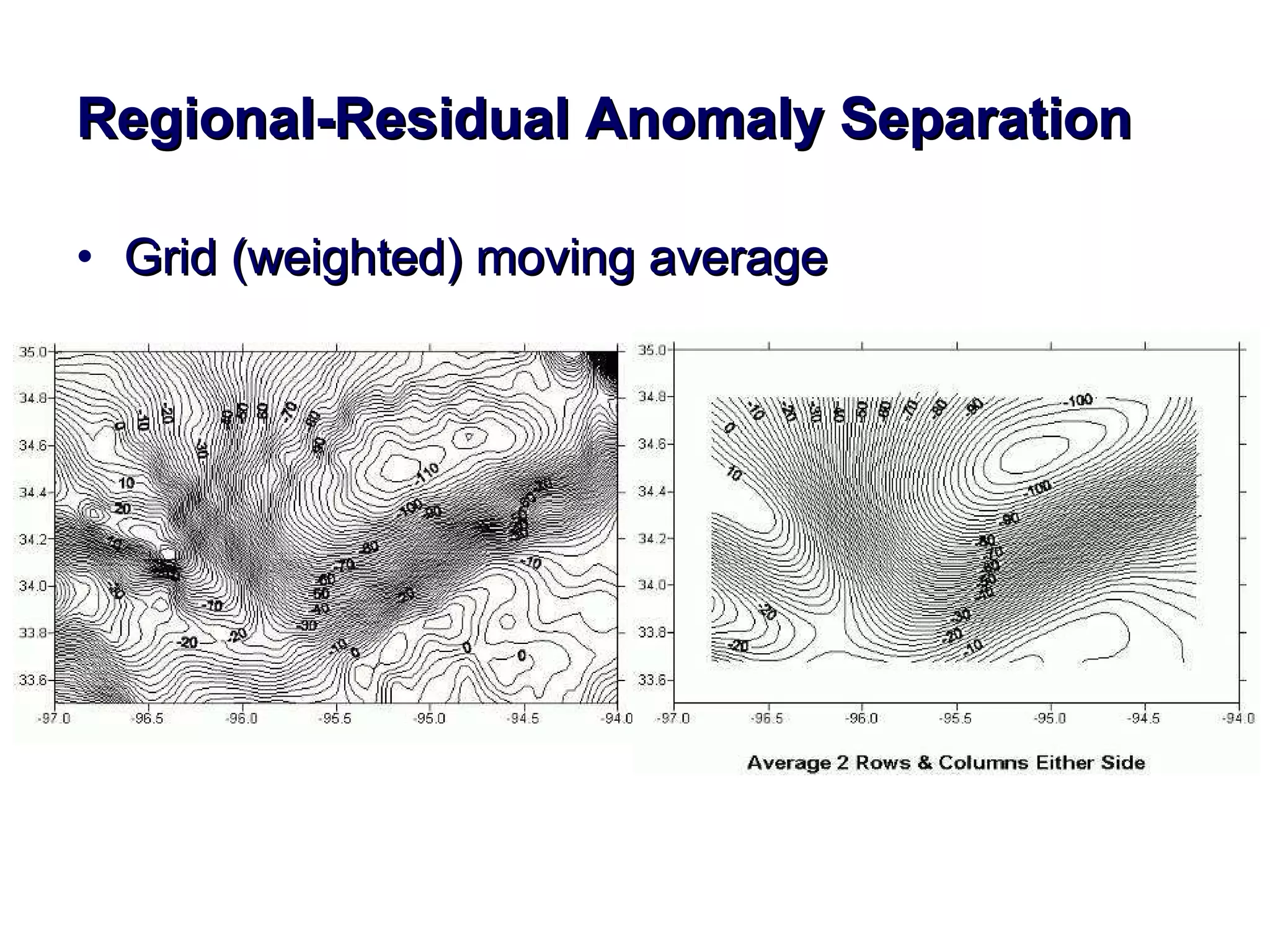
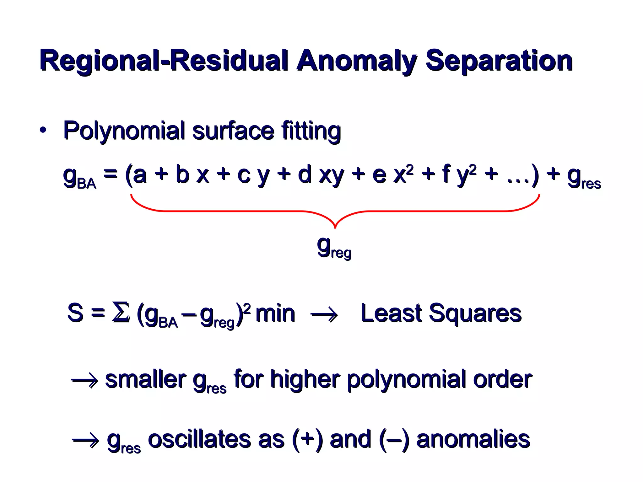
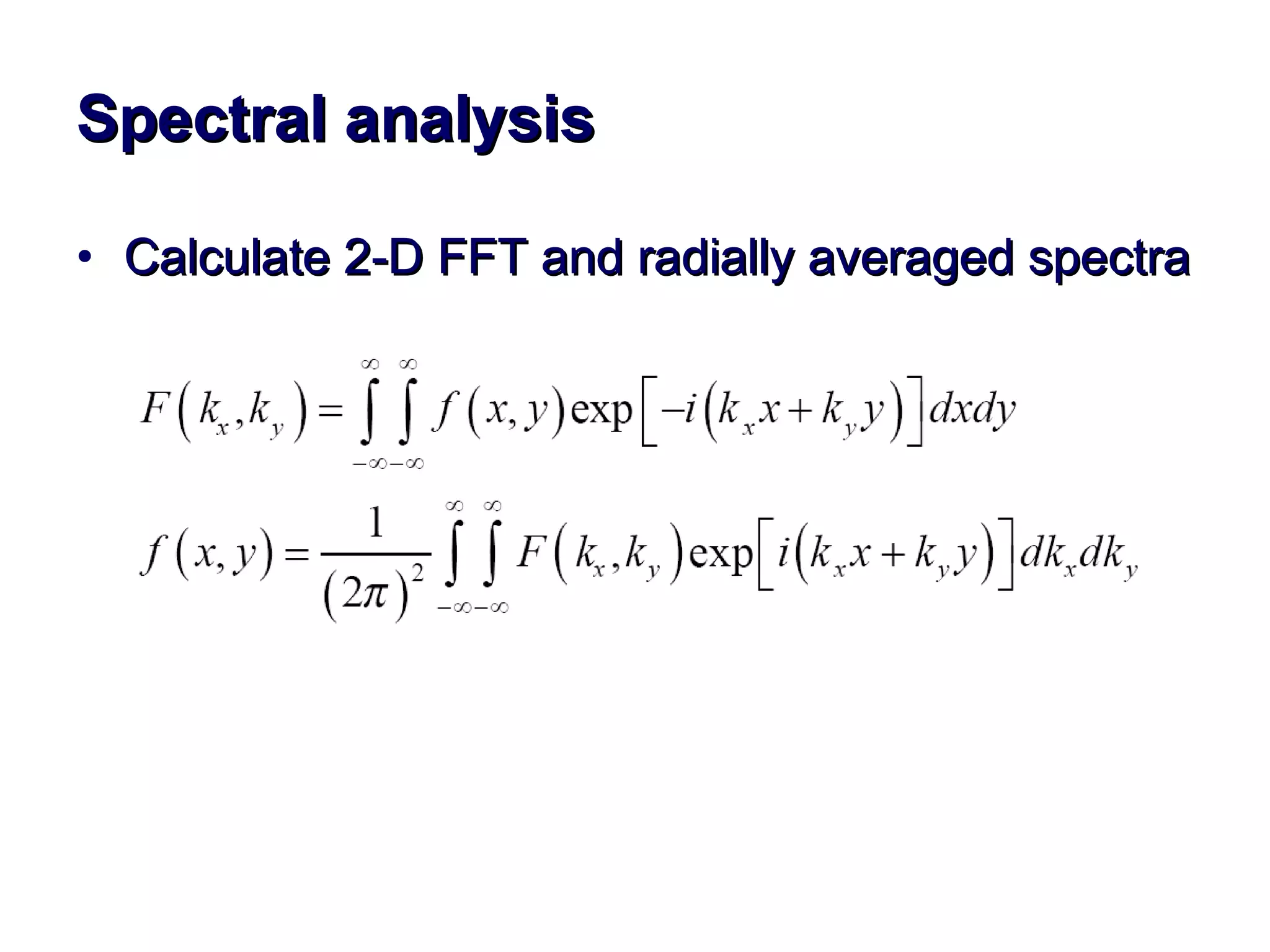
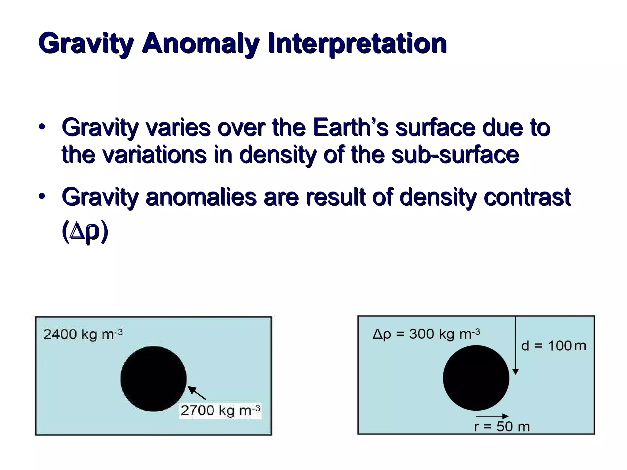
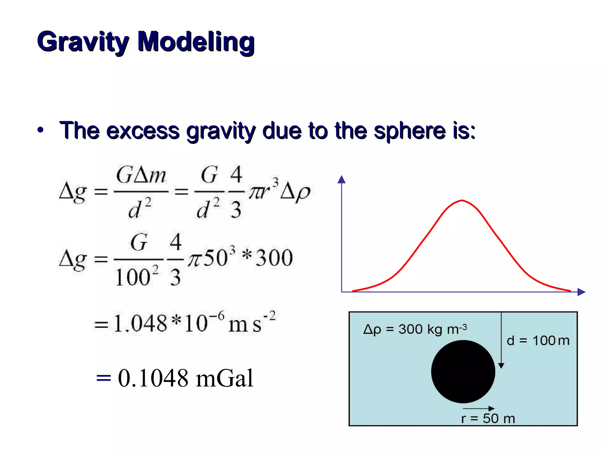
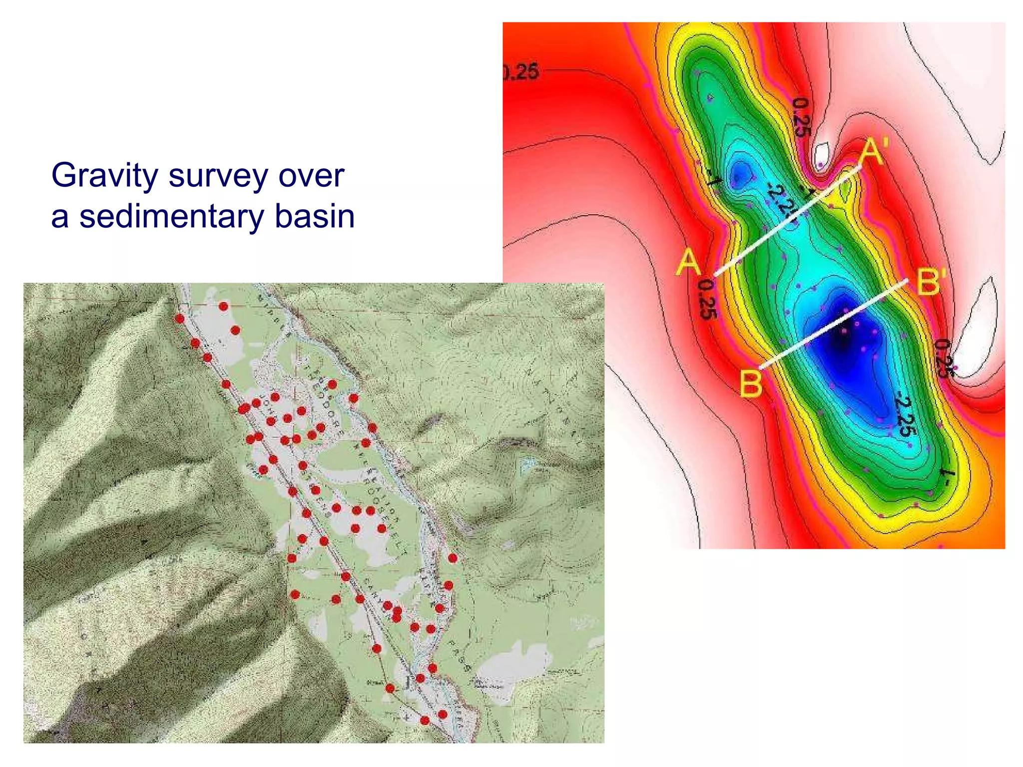
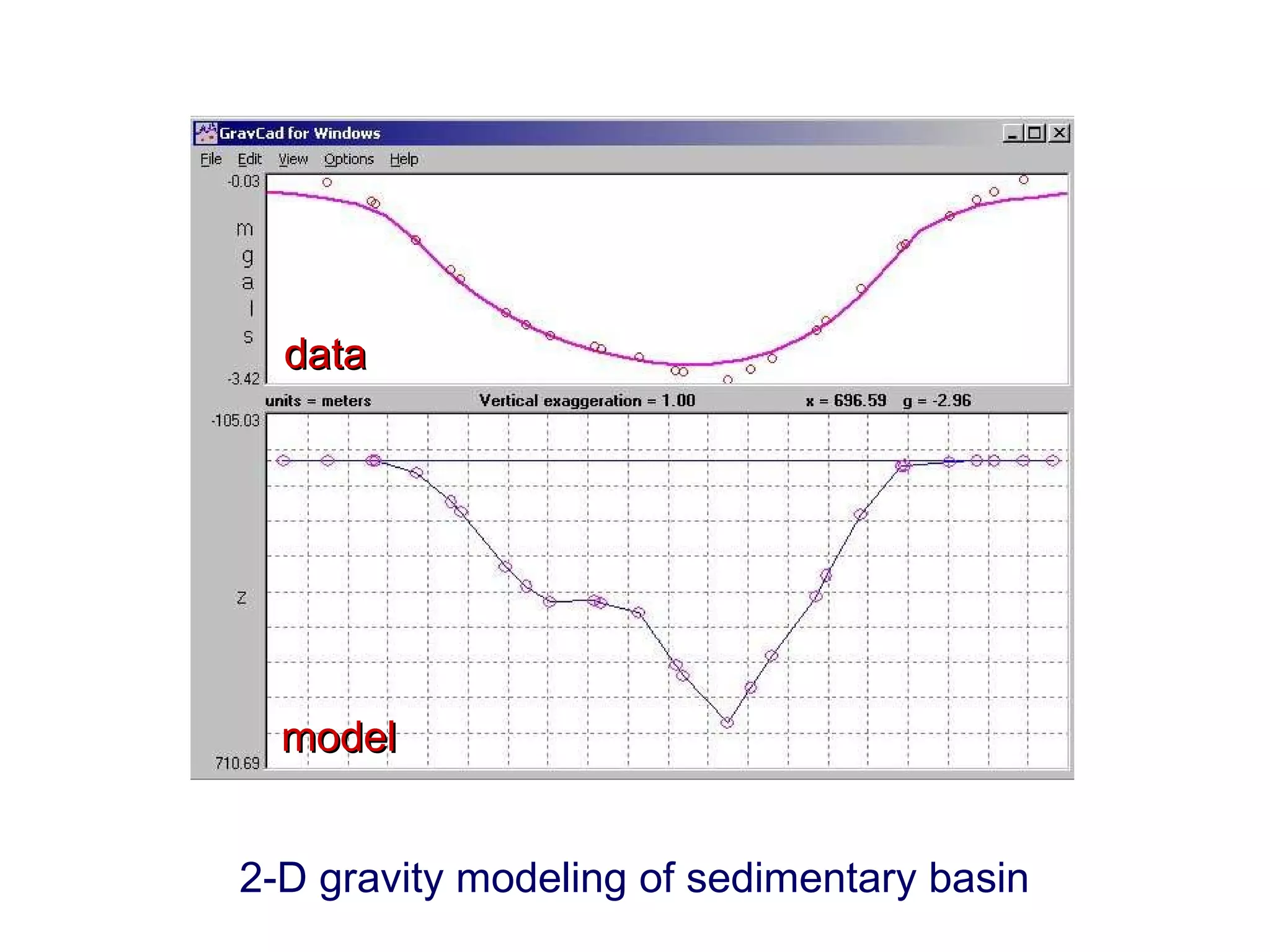
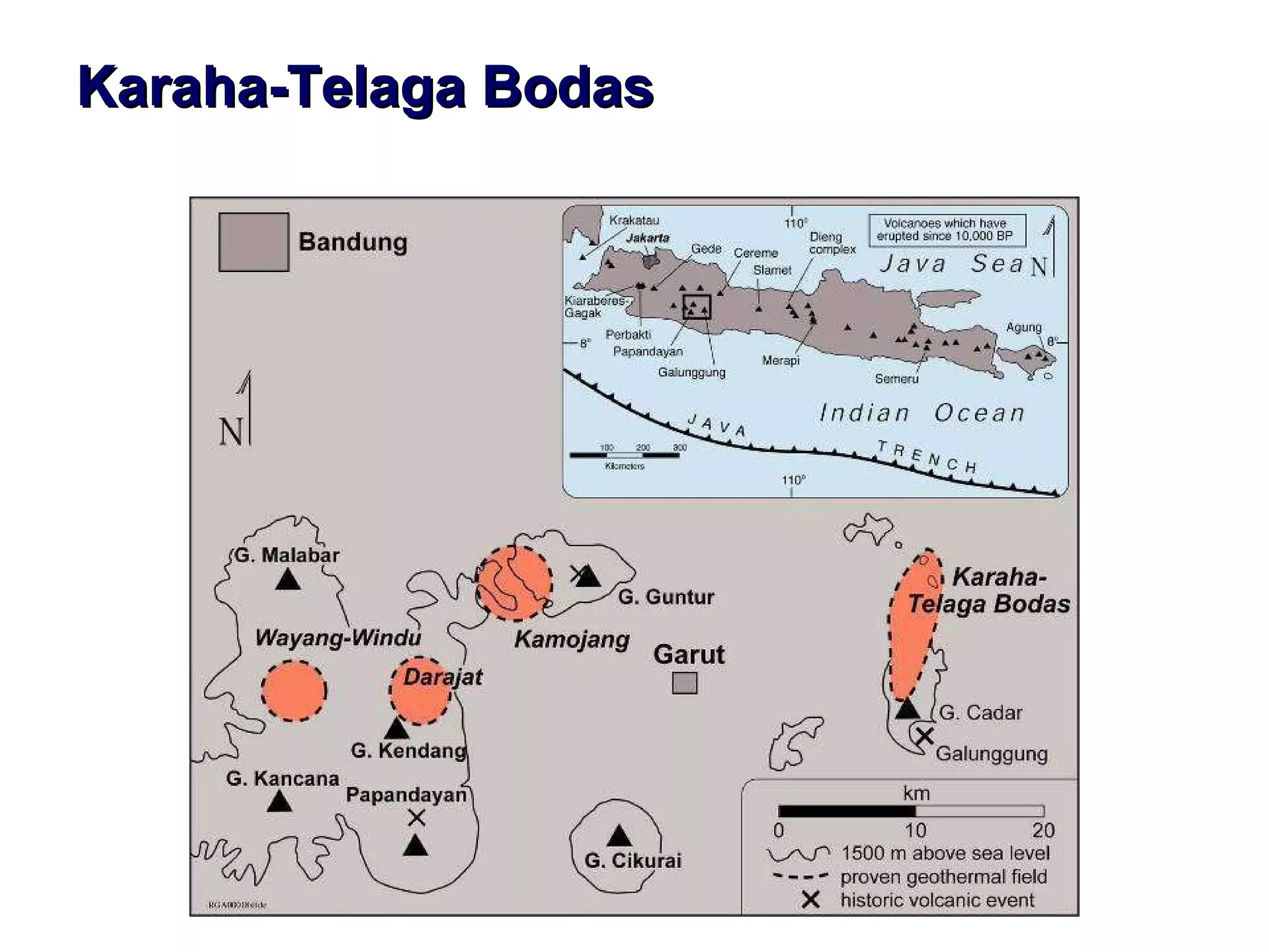
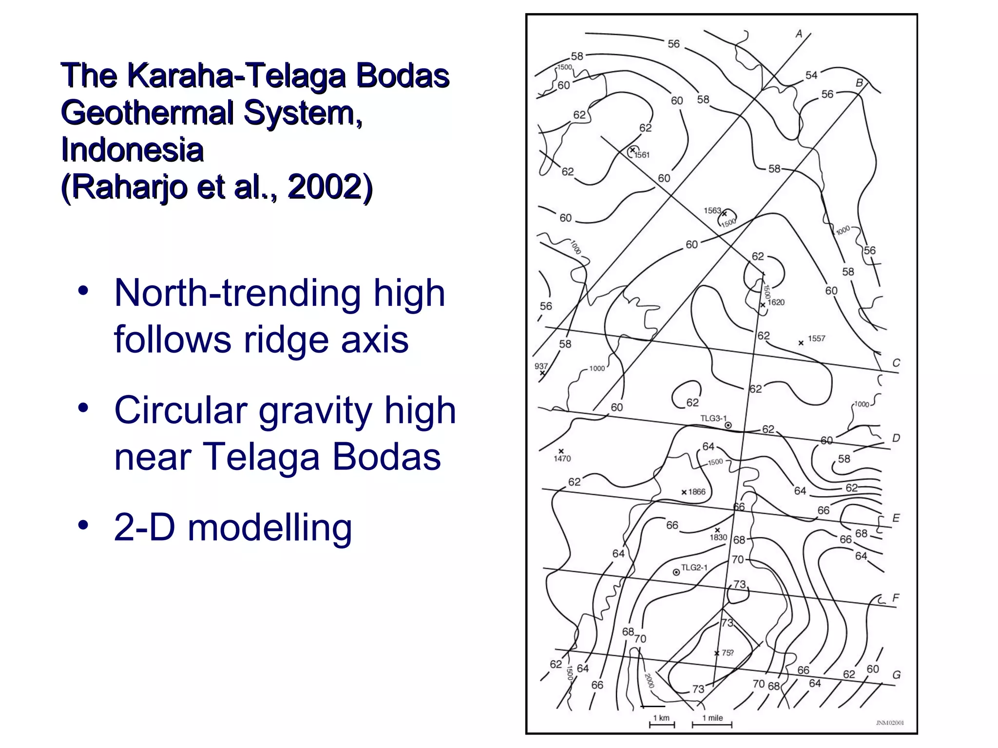
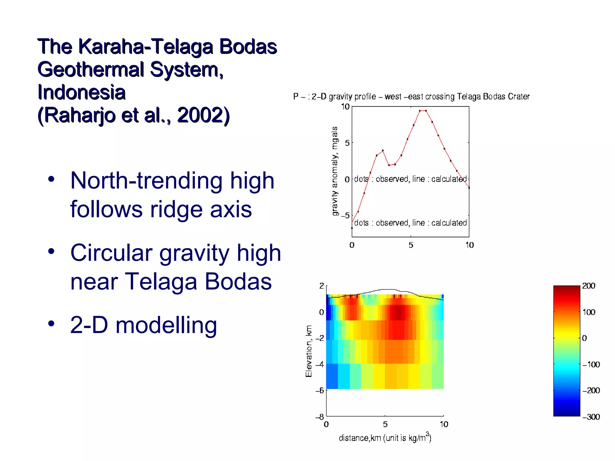
This document discusses magnetic and gravity methods for geothermal exploration. It provides an overview of how magnetic and gravity surveys are conducted, including the equipment used and data processing techniques. It also describes how potential field data can be used to infer subsurface structures and aid in geological interpretation and 3D modeling of geothermal prospects.

1. Magnetic and Gravity Methods for Geothermal Exploration Dr. Hendra Grandis Geophysics - ITB

2. Ql : existence of deep structure, i.e. intrusive body or caldera structures Qt : geometry of those above (the upper structure must be closely defined) high or low anomaly gravity (covers low and high magnetic areas) Ql : ascending thermal fluid (and / or descending cold water) Qt : ? high or low anomaly self-potential (across high and low resistivity areas) Ql : can be associated with thermal fluids upflow and outflow zones Qt : shallow resistivity structure low anomaly Schlumberger resistivity mapping and sounding (concentrated in the area between broad magnetic low and high) Ql : can be associated with thermally altered zones Qt : geometry (?) low anomaly Aero- or ground magnetic (covers a large area) interpretation expected anomaly method and survey procedure

3. Probable sequence of geophysical exploration methods used to investigate young volcanic geothermal prospect (revised from Sudarman, 1983) Ql : permeable zones Qt : ? high anomaly micro-seismics (M< 3) Ql : can be associated with thermal fluids upflow and outflow zones Qt : deeper resistivity structure low anomaly Magnetotelluric sounding Ql : uprising or horisontal thermal fluid movement, if depth to resevoir is relatively shallow Qt : defined the upper structure high anomaly Thermal gradient and anomalous temperature (to figure out the cause of low resistivity layer) interpretation expected anomaly method and survey procedure

4. Magnetic Method Covers large area as regional reconnaissance (aero-mag, + remote sensing) More local coverage (ground-mag) to search for demagnetized bodies associated with thermally altered zones Precaution for dipolar nature of magnetic anomalies Advanced processing for anomaly enhancement and modeling

5. Aero-magnetic Survey

6. aero-magnetic data and interpretation

7. Ground-magnetic Survey

8. Vectors of the Earth’s magnetic field

9. Dipolar anomaly related to inclined inducing main magnetic field

10. Typical magnetic anomaly at low latitudes

11. Anomaly detected in N-S traverse over E-W anomalous body

12. Reduction to Equator and Pole of Magnetic data Frequency domain filtering process

13. Spectral analysis Depth and spatial extent of the anomalous sources are related to frequency or wavelength of the data low frequency / long wavelength ~ deep and regional anomalies high frequency / short wavelength ~ shallow and local anomalies information on depth of anomalous sources can be obtained from spectral analysis of potential filed data

14. Wavelength or frequency and anomaly’s depth

15. Spectral analysis Calculate 2-D FFT and radially averaged spectra relationship between slope of power spectrum with depth filtering (low-pass, high-pass, band-pass) regional – residual anomaly separation pseudo-depth slicing

16. Radially averaged spectra and line-fitted segments

17. Softwares for magnetic data processing and modeling

18. Kamojang (Sungkono & Hochstein, 1995)

19. Wairakei, NZ (Sungkono & Hochstein, 1995)

20. Gravity method g 1 g 2 g 3 distance g gravity data

21. Gravity Measurement We try to obtain exess or deficiency of gravity relative to “normal” gravity  gravity anomaly  difference between observed gravity and normal or theoretical gravity g ANOMALY = g OBSERVED - g THEORY   must be corrected from factors affecting them

22. Observed Gravity Use of relative gravimeter  only measure the difference of gravity values between two places  measure gravity values at gravity stations relative to gravity base station (BS) BS St-1  R = R2 – R1   g 1 = g BS +  R R1 R2  known

23. Gravity Base Station Local Base Station  all stations’ gravity values are relative to this local Base Station  tied or referenced to a higher order gravity Base Station (regional, national)  used for drift correction

25. Factors Affecting Observed Gravity Instrumental drift correction determined by looping procedure, i.e base station measurement at the beginning and at the end of a survey

26. Gravity Anomaly g ANOMALY = g OBSERVED – g THEORY g OBSERVED  gravity value relative to a known base station g THEORY  Gravity Reference Field (GRF) corrected to meet the observation condition ( elevation  MSL )  corrections: Free-Air, Bouguer, Terrain

28. Gravity Data Processing Data Reduction Field gravity measurements must be corrected to account for several factors which effect the readings, also known as “reducing the data” Solid earth’s tide Instrumental drift Field readings  Station’s Gravity (g obs ) (relative to a known Base)

29. G r a v i t y D a t a P r o c e s s i n g Gravity Correction Station’s Gravity must be corrected such that the values represent a perfect homogenous sphere, called a “geoid”. If there are still differences in the readings after the corrections are made, then they may truly represent a gravity anomaly. Corrections Latitude, Free-air, Bouguer, Terrain

30. Gravity Correction Latitude correction Normal Gravity from International Gravity Formula 1967 g N (  ) = 9.78031846 (1 + 0.0053024 sin 2    – 0.0000058 sin 2 2  ) g N (  ) represents theoretical gravity at sea-level (reference),  = latitude

31. Gravity Correction Free-air correction To compensate the height of gravity stations above sea-level (level of reference) g FA  – 0.3086 × h A MSL h

32. Gravity Correction Bouguer correction To compensate the rock mass between sea-level to station’s elevation (level of reference). g B  + 0.04193 ×  × h  Bouguer slab formula A MSL h

33. Gravity Correction Terrain correction To compensate the topography: existence of rock mass of hills (M1) and the inexistence of rock-mass in valleys (M2) g TC are obtained from table or calculated A M1 M2 MSL

34. Gravity Correction Terrain correction M1 will decrease gravity value at A (negative vertical attraction), Bouguer correction considers that there is M2 so mass attraction equivalent to M2 must be extracted from values at A A M1 M2 MSL

35. Bouguer Anomaly Gravity corrections are applied to g N (  ), i.e. theoretical gravity at reference-level, to obtain theoretical gravity values at measurement stations g theor  g N (  ) – g FA + g B – g TC Bouguer Anomaly is the difference between observed Gravity and theoretical gravity g BA  g obs – g theor  g obs – g N (  ) + g FA – g B + g TC

36. Bouguer Anomaly Gravity corrections do not bring (reduce) gravity values from stations’ elevation to the reference / sea-level Bouguer anomalies are values at stations’ elevation (A), not values at reference / sea- level A MSL h

37. Regional-Residual Anomaly Separation Free-hand smoothing Grid (weighted) moving average Second Vertical Derivative (SVD) Polynomial surface fitting Spectral analysis – based filtering Qualitative vs. Quantitative Anomaly enhancement

38. Regional-Residual Anomaly Separation Free-hand smoothing Profile Map

39. Regional-Residual Anomaly Separation Grid (weighted) moving average  related to SVD

40. Regional-Residual Anomaly Separation Second Vertical Derivative (SVD)

41. Regional-Residual Anomaly Separation Grid (weighted) moving average

42. Regional-Residual Anomaly Separation Polynomial surface fitting g BA = (a + b x + c y + d xy + e x 2 + f y 2 + …) + g res g reg S =  (g BA – g reg ) 2 min  Least Squares  smaller g res for higher polynomial order  g res oscillates as (+) and (–) anomalies

43. Spectral analysis Calculate 2-D FFT and radially averaged spectra

44. Radially averaged spectra and line-fitted segments

45. Gravity Anomaly Interpretation Gravity varies over the Earth’s surface due to the variations in density of the sub-surface Gravity anomalies are result of density contrast (   )

46. Gravity Modeling The excess gravity due to the sphere is: = 0.1048 mGal

47. Gravity survey over a sedimentary basin

48. 2-D gravity modeling of sedimentary basin data model

49. Karaha-Telaga Bodas

50. The Karaha-Telaga Bodas Geothermal System, Indonesia (Raharjo et al., 2002) North-trending high follows ridge axis Circular gravity high near Telaga Bodas 2-D modelling

51. The Karaha-Telaga Bodas Geothermal System, Indonesia (Raharjo et al., 2002) North-trending high follows ridge axis Circular gravity high near Telaga Bodas 2-D modelling