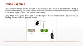
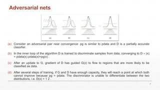
Download to read offline
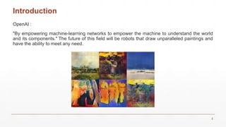
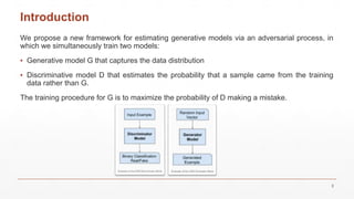
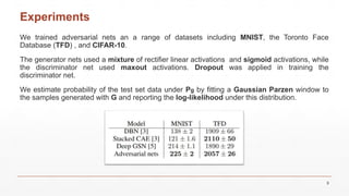
This document introduces Generative Adversarial Networks (GANs), which consist of a generative model that captures data distribution and a discriminative model that distinguishes real data from generated data. It discusses the training process and comparisons with adversarial examples, while highlighting the advantages and disadvantages of the GAN framework. The document also describes experiments conducted on datasets such as MNIST and CIFAR-10, illustrating the generator's ability to create realistic images over time.


![[Paper] GIRAFFE: Representing Scenes as Compositional Generative Neural Featu...](https://cdn.slidesharecdn.com/ss_thumbnails/papergirafferepresentingscenesascompositionalgenerativeneuralfeaturefields-210823043723-thumbnail.jpg?width=640&height=640&fit=bounds)