This document discusses generative adversarial networks (GANs) for generating synthetic images that are indistinguishable from real images. It introduces GANs, explaining how they involve two neural networks - a generator that produces synthetic images and a discriminator that evaluates them as real or fake. The networks are trained in an adversarial process, with the generator trying to fool the discriminator and the discriminator trying to distinguish real from fake images. The document outlines the GAN training process and theoretical guarantees, provides experimental results on image datasets, and discusses advantages, disadvantages and potential future applications of GANs.

1. YANJUN WU
Network Science Lab
Dept. of Artificial Intelligence
The Catholic University of Korea
E-mail:wuyanjun@catholic.ac.kr

2. 1
1. Introduction
evolve predator
Eaten
Not eaten
We know that there are many kinds of butterflies, and one of them is like a dead leaf.
In order not to be eaten by predators, it slowly evolved to look like a dead leaf. Finally,
it becomes difficult for predators to distinguish between a fallen leaf and a butterfly.

3. 2
1. Introduction
z
G
G(z)
X
D
D(X):The probability that the discriminator considers x is a true image.
D(G(z)):The probability that the discriminator considers the fake image to be a true image.
The fake image is trained hard to make the discriminator think it is the real image.
The final goal is that the discriminator will not be able to distinguish between true and false images
generated by the generator.
D(X)
D(G(z))

4. 3
2. Adversarial nets
Understanding the Loss Function
Ex∼pdata ​(x)​：x is a sample from the real data distribution P .
Ez∼pz​(z)​： z is the sample that generates the data distribution Z.
When the image satisfies the true image distribution we use
When the image satisfies the false image distribution we use
D is trying to figure out how to increase the value of V.
G is trying to figure out how to decrease the value of V.
They are fighting against each other.

5. 4
2. Adversarial nets
1) Fixed G training D
The purpose of training D is to hope that V is as big as possible.
Real data wants to be predicted as 1 and generated data wants to be predicted as 0.
We first train the discriminator (D), and we want the discriminator to think that the
probability that the true image is the true image is as high as possible. So expect D
(x) to be close to 1. We want the discriminator to think that the probability that the
false image is the true image is as small as possible. So expect D(G(z)) to be close
to 0.
After this step we get D, so D(X) is fixed

6. 5
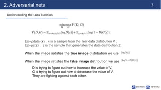
2. Adversarial nets
2) Fixed D, Training G
It is hoping that the value of V is as small as possible so that D cannot distinguish
between true and false data.
Because we have trained D, it is D constant, so it can be just ignored unaffected.
It is expected that the discriminator thinks that the probability that the false image is
the true image is as large as possible. So expect D(G(z)) to be close to 1. So expect
log[1-D(G(z))] to be close to 0.

7. 6
2. Adversarial nets
Train the discriminator k times, at which point t
he generator fixes
1. sample m noises to generate m false images
G(z)
2. sample m true images
3. update the discriminator weights from the loss
function and gradient (train the binary classific
ation loss function with the fake and true imag
es)
Train the generator once, when the discriminat
or is fixed
1. sample m noises to generate m fake images
2. update generator weights from loss function
and gradient

8. 7
2. Adversarial nets
Z is noise, a uniformly distributed random number
Blue line: Probability that the discriminator predicts x to be the real image
Green line: generator produces image distribution Pz
Black line: probability of real image distribution Px
real image space
fake image
Noise space (uniformly distributed random numbers)
Generator(G)
Training discriminator D The training generator G Training n times
Real image distribution Px
=
Generated image distribution Pz
D(x)
The discriminator is
completely unable to
distinguish between
the two distributions
D（x）= 0.5
Global Optimality of
Pz = px

9. 8
3. Theoretical Results
Given any generator G, train the discriminator D and maximize V
G fixed, the optimal discriminator D

10. 9
3. Theoretical Results
We already know the best performance of D. The case in which G wants to get
the best solution in this case is that
The global minimum of the virtual training criterion C(G) is achieved if and only
if . At that point, C(G) achieves the value − log 4

11. 10
4. Experiments
Different standard models are used to generate the images and
higher scores show that the generated data is more realistic.
We can see that it scores high on MINST dataset. But the score
is not the highest on TFD dataset. But it is another method with
unlimited potential.

12. 11
5. Experiments
The image in the yellow box is the generated image and we can notice that
it is the generated image it creates itself.
original sample
This row represents the training samples that are closest to the generated image

13. 12
5. Advantages and disadvantages
Advantages:
1.Does not require Markov chains, uses only backward propagation to obtain gradients,
does not require inference during learning, and can combine more than one function into
the model.
2.The generator network is not updated directly using data examples, but only using the
gradient of the discriminator.
3.Data distributions using GANs can be sharp (e.g., Gaussian), but distributions using
Markov chain data must be smooth.
Disadvantage:
1.We don't know what the sample distribution of the original data looks like and can’t
express it in a formula.
2.And the discriminator must be trained in the same time as the generator (in particular,
you can't train G too much without updating D)

14. 13
6. Conclusions and future work
1. conditional GAN. tell it to generate the class that generates the picture.
2. introduce an auxiliary network input a picture and predict the noise.
3. image fill (remove objects from specified area and fill with other)
Super resolution (blurred image to generate high definition image)
4. for semi-supervised learning to improve the case of few labels
5. improve the loss function to speed up training

15. 14
5. Question
Q&A