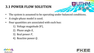
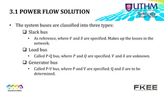
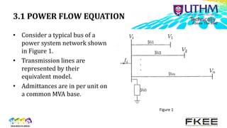
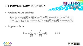
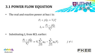
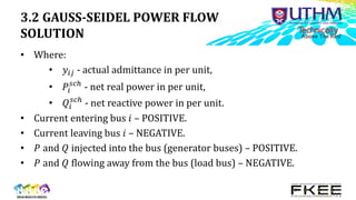
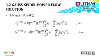
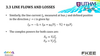
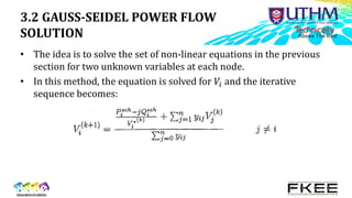
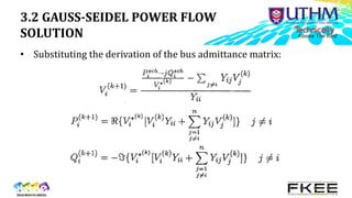
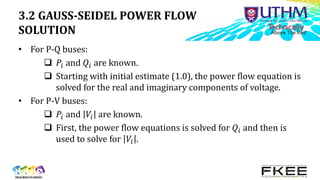
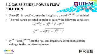
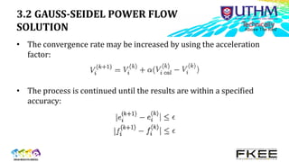
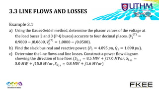
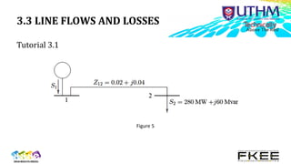
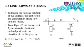
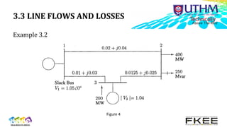
The document describes power flow analysis and the Gauss-Seidel method for solving power flows. It discusses: 1) Power flow equations relating voltage, current, real and reactive power at each bus. 2) The Gauss-Seidel method iteratively solves these nonlinear equations to determine voltage phasors and power flows. 3) Line flows and losses are then calculated using the bus voltages and currents based on admittance matrices. 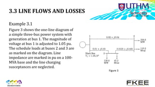Examples and tutorials demonstrate applying the method to simple systems.

1. BEF43303
POWER SYSTEM ANALYSIS AND
PROTECTION
POWER FLOW ANALYSIS
WEEK 3

2. 3.0 CONTENTS
3.1 Power flow solution
3.2 Gauss-Seidel power flow solution
3.3 Line flows and losses

3. 3.1 POWER FLOW SOLUTION
• The system is assumed to be operating under balanced conditions.
• A single-phase model is used.
• Four quantities are associated with each bus:
1) Voltage magnitude 𝑉 ,
2) Phase angle 𝛿,
3) Real power 𝑃,
4) Reactive power 𝑄.

4. 3.1 POWER FLOW SOLUTION
• The system buses are classified into three types:
 Slack bus
• As reference, where 𝑉 and 𝛿 are specified. Makes up the losses in the
network.
 Load bus
• Called P-Q bus, where 𝑃 and 𝑄 are specified. 𝑉 and 𝛿 are unknown.
 Generator bus
• Called P-V bus, where P and V are specified. Q and 𝛿 are to be
determined.

5. 3.1 POWER FLOW EQUATION
• Consider a typical bus of a
power system network shown
in Figure 1.
• Transmission lines are
represented by their
equivalent model.
• Admittances are in per unit on
a common MVA base.
Figure 1

6. 3.1 POWER FLOW EQUATION
• Applying KCL to this bus:
• In general form:

7. 3.1 POWER FLOW EQUATION
• The real and reactive power at bus 𝑖 is:
• Substituting 𝐼𝑖 from KCL earlier:

8. 3.2 GAUSS-SEIDEL POWER FLOW
SOLUTION
• The idea is to solve the set of non-linear equations in the previous
section for two unknown variables at each node.
• In this method, the equation is solved for 𝑉𝑖 and the iterative
sequence becomes:

9. 3.2 GAUSS-SEIDEL POWER FLOW
SOLUTION
• Where:
• 𝑦𝑖𝑗 - actual admittance in per unit,
• 𝑃𝑖
𝑠𝑐ℎ
- net real power in per unit,
• 𝑄𝑖
𝑠𝑐ℎ
- net reactive power in per unit.
• Current entering bus 𝑖 – POSITIVE.
• Current leaving bus 𝑖 – NEGATIVE.
• 𝑃 and 𝑄 injected into the bus (generator buses) – POSITIVE.
• 𝑃 and 𝑄 flowing away from the bus (load bus) – NEGATIVE.

10. 3.2 GAUSS-SEIDEL POWER FLOW
SOLUTION
• Solving for 𝑃𝑖 and 𝑄𝑖:

11. 3.2 GAUSS-SEIDEL POWER FLOW
SOLUTION
• Substituting the derivation of the bus admittance matrix:

12. 3.2 GAUSS-SEIDEL POWER FLOW
SOLUTION
• For P-Q buses:
 𝑃𝑖 and 𝑄𝑖 are known.
 Starting with initial estimate (1.0), the power flow equation is
solved for the real and imaginary components of voltage.
• For P-V buses:
 𝑃𝑖 and 𝑉𝑖 are known.
 First, the power flow equations is solved for 𝑄𝑖 and then is
used to solve for 𝑉𝑖 .

13. 3.2 GAUSS-SEIDEL POWER FLOW
SOLUTION
• Since 𝑉𝑖 is specified, only the imaginary part of 𝑉
𝑖
(𝑘+1)
is retained.
• The real part is selected in order to satisfy the following condition:
• 𝑒𝑖
(𝑘+1)
and 𝑓𝑖
(𝑘+1)
are the real and imaginary components of the
voltage in the iterative sequence.

14. 3.2 GAUSS-SEIDEL POWER FLOW
SOLUTION
• The convergence rate may be increased by using the acceleration
factor:
• The process is continued until the results are within a specified
accuracy:

15. 3.2 GAUSS-SEIDEL POWER FLOW
SOLUTION
• A voltage accuracy in the range of 0.00001 and 0.00005 pu is
satisfactory.
• In practice, the power mismatch is used as the stopping criteria.
• A typical power mismatch accuracy is 0.001 pu.

16. 3.3 LINE FLOWS AND LOSSES
• Following the iterative solution
of bus voltages, the next step is
the computation of line flow
and line losses.
• From Figure 2, the line current
𝐼𝑖𝑗, measured at bus 𝑖 and
defined positive in the
direction of 𝑖 → 𝑗 is given by:
Figure 2

17. 3.3 LINE FLOWS AND LOSSES
• Similarly, the line current 𝐼𝑗𝑖 measured at bus 𝑗 and defined positive
in the direction 𝑗 → 𝑖 is given by:
• The complex powers for both cases are:

18. 3.3 LINE FLOWS AND LOSSES
• The power loss in line 𝑖 − 𝑗 is the algebraic sum of the power flows
given as follows:

19. 3.3 LINE FLOWS AND LOSSES
Example 3.1
Figure 3 shows the one-line diagram of
a simple three-bus power system with
generation at bus 1. The magnitude of
voltage at bus 1 is adjusted to 1.05 pu.
The schedule loads at buses 2 and 3 are
as marked on the diagram. Line
impedance are marked in pu on a 100-
MVA base and the line charging
susceptances are neglected.
Figure 3

20. 3.3 LINE FLOWS AND LOSSES
Example 3.1
a) Using the Gauss-Seidel method, determine the phasor values of the voltage at
the load buses 2 and 3 (P-Q buses) accurate to four decimal places. (𝑉
2
(7)
=
0.9800 − 𝑗0.0600, 𝑉
3
(7)
= 1.0000 − 𝑗0.0500).
b) Find the slack bus real and reactive power. (𝑃1 = 4.095 𝑝𝑢, 𝑄1 = 1.890 𝑝𝑢).
c) Determine the line flows and line losses. Construct a power flow diagram
showing the direction of line flow. (𝑆𝐿12
= 8.5 𝑀𝑊 + 𝑗17.0 𝑀𝑉𝑎𝑟, 𝑆𝐿13
=
5.0 𝑀𝑊 + 𝑗15.0 𝑀𝑉𝑎𝑟, 𝑆𝐿23
= 0.8 𝑀𝑊 + 𝑗1.6 𝑀𝑉𝑎𝑟)

21. 3.3 LINE FLOWS AND LOSSES
Example 3.2
Figure 4 shows the one-line diagram of a simple three-bus power system with
generators at bus 1 and 3. The magnitude of voltage at bus 1 is adjusted to 1.05 pu.
Voltage magnitude at bus 3 is fixed at 1.04 pu with real power generation of 200
MW. A load consisting of 400 MW and 250 MVar is taken from bus 2. Line
impedance are marked in per unit on a 100 MVA base, and the line charging
susceptances are neglected. Obtain the power flow solution by the Gauss-Seidel
method including line flows and line losses. (𝑉2 = 0.97168∠ −2.6948°
pu, 𝑆3 =
2.0 + 𝑗1.4617 pu, 𝑉3 = 1.04∠ −0.498° pu, 𝑆1 = 2.1842 + 𝑗1.4085 pu, 𝑆𝐿12
= 8.39 +
𝑗16.79 MVA, 𝑆𝐿13
= 0.18 + 𝑗0.548 MVA, 𝑆𝐿23
= 9.85 + 𝑗19.69 MVA).

22. 3.3 LINE FLOWS AND LOSSES
Example 3.2
Figure 4

23. 3.3 LINE FLOWS AND LOSSES
Example 3.2
Figure 4 shows the one-line diagram of a simple three-bus power system with
generators at bus 1 and 3. The magnitude of voltage at bus 1 is adjusted to 1.05 pu.
Voltage magnitude at bus 3 is fixed at 1.04 pu with real power generation of 200
MW. A load consisting of 400 MW and 250 MVar is taken from bus 2. Line
impedance are marked in per unit on a 100 MVA base, and the line charging
susceptances are neglected. Obtain the power flow solution by the Gauss-Seidel
method including line flows and line losses. (𝑉2 = 0.97168∠ −2.6948°
pu, 𝑆3 =
2.0 + 𝑗1.4617 pu, 𝑉3 = 1.04∠ −0.498° pu, 𝑆1 = 2.1842 + 𝑗1.4085 pu, 𝑆𝐿12
= 8.39 +
𝑗16.79 MVA, 𝑆𝐿13
= 0.18 + 𝑗0.548 MVA, 𝑆𝐿23
= 9.85 + 𝑗19.69 MVA).

24. 3.3 LINE FLOWS AND LOSSES
Example 3.2
Figure 4

25. 3.3 LINE FLOWS AND LOSSES
Tutorial 3.1
In the power system network shown in Figure 5, bus 1 is a slack bus with 𝑉1 =
1.06∠0°pu and bus 2 is a load bus with 𝑆2 = 280 + 𝑗60 MVA. The line impedance
on a base of 100 MVA is 0.02 + 𝑗0.04 pu.
a) Using Gauss-Seidel method, determine 𝑉2. Use an initial estimate of 𝑉
2
(0)
=
1.0 + 𝑗0.0 and perform four iterations. (0.90 − 𝑗0.10 pu).
b) If after several iterations voltage at bus 2 converges to 𝑉2 = 0.90 − 𝑗0.10 pu
determine 𝑆1 and the real and reactive power loss in the line. (20 + 𝑗40 MVA).

26. 3.3 LINE FLOWS AND LOSSES
Tutorial 3.1
Figure 5

27. 3.3 LINE FLOWS AND LOSSES
Tutorial 3.2
Figure 6 shows the one-line diagram of a simple three-bus power system with generation at bus 1.
The voltage at bus 1 is 𝑉1 = 1.06∠0°pu. The scheduled loads on buses 2 and 3 are marked on the
diagram. Line impedances are marked in pu on a 100 MVA base. For the purpose of hand
calculations, line resistances and line charging susceptances are neglected.
a) Using Gauss-Seidel method and initial estimates of 𝑉
2
(0)
= 1.0 + 𝑗0.0 and 𝑉
3
(0)
= 1.0 + 𝑗0.0,
determine 𝑉2 and 𝑉3. Perform two iterations. (0.9089 − 𝑗0.0974 pu, 0.9522 − 𝑗0.0493)
b) If after several iterations the bus voltages converge to:
𝑉2 = 0.90 − 𝑗0.10 pu
𝑉3 = 0.95 − 𝑗0.05 pu
determine the line flows and line losses and the slack bus real and reactive power. (7.0 − 𝑗7.0,
𝑗60, 𝑗40, 𝑗10).

28. 3.3 LINE FLOWS AND LOSSES
Tutorial 3.2
Figure 6

29. 3.3 LINE FLOWS AND LOSSES
Tutorial 3.3
Figure 7 shows the one-line diagram of a simple three-bus power system with generation at buses 1 and 3. The
voltage at bus 1 is 𝑉1 = 1.025∠0°pu. Voltage magnitude at bus 3 is fixed at 1.03 pu with a real power
generation of 300 MW. A load consisting of 400 MW and 200 MVar is taken from bus 2. Line impedances are
marked in per unit on a 100 MVA base. For the purpose of hand calculations,
line resistances and line charging susceptances are neglected.
a) Using Gauss-Seidel method and initial estimates of 𝑉
2
(0)
= 1.0 + 𝑗0.0 and 𝑉
3
(0)
= 1.03 + 𝑗0.0 and keeping
𝑉3 = 1.03 pu, determine the phasor values of 𝑉2 and 𝑉3. Perform two iterations. (1.0001 − 𝑗0.0409 pu,
1.3671 pu, 1.0298 + 𝑗0.0216 pu).
b) If after several iterations the bus voltages converge to:
𝑉2 = 1.000571 − 𝑗0.0366898 pu
𝑉3 = 1.029706 + j0.0246 pu
determine the line flows and line losses and the slack bus real and reactive power. (100 + 𝑗90.51 MVA,
𝑗7.77 MVA, 𝑗1.25 MVA, 𝑗18.42 MVA).

30. 3.3 LINE FLOWS AND LOSSES
Tutorial 3.3
Figure 7