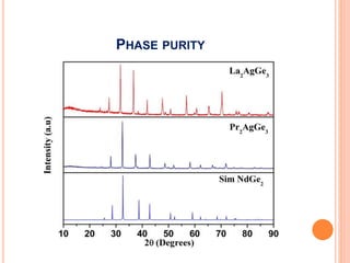
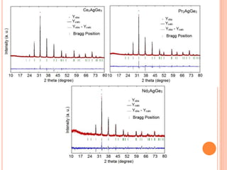
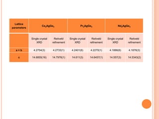
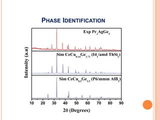
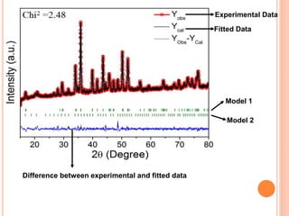
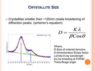
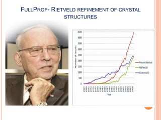
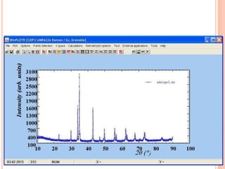
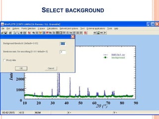
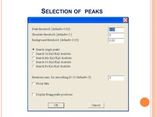
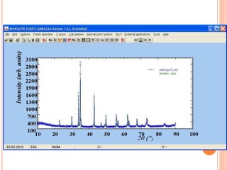
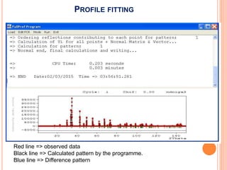
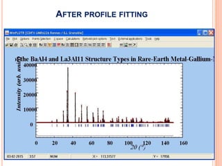
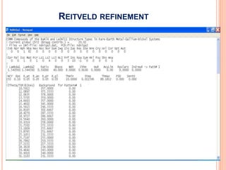
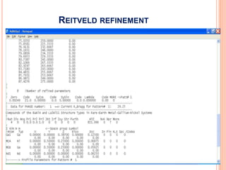
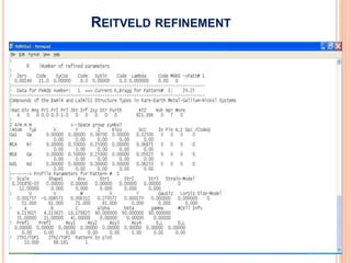
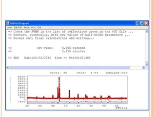
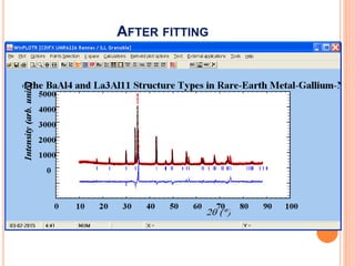
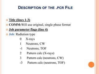
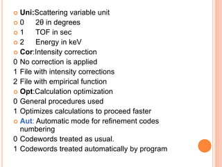
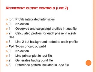
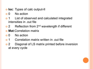
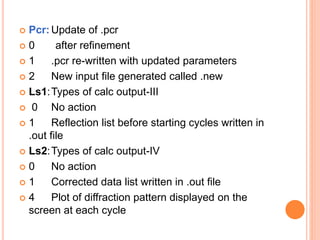
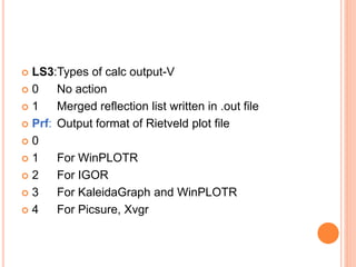
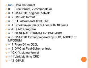
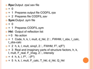
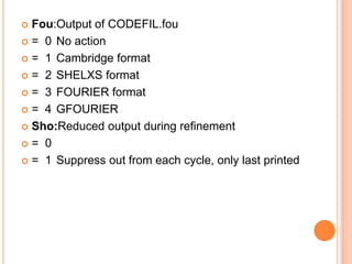
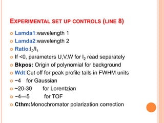
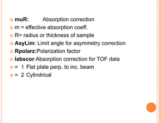
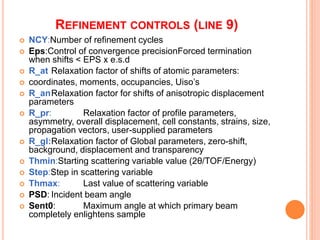
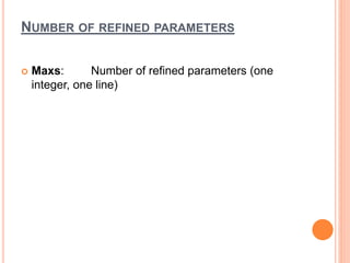
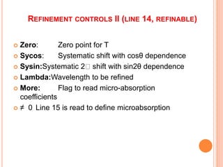
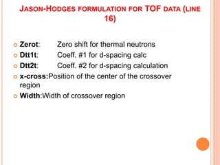
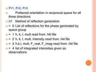
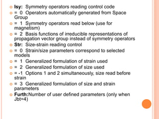
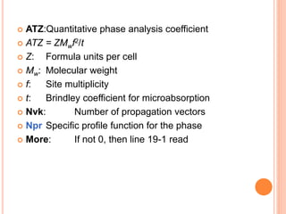
The document discusses the use of Rietveld refinement for analyzing powder X-ray diffraction data. Rietveld refinement allows for the determination of phase purity, identification of crystal structures, refinement of structural parameters, quantitative phase analysis, and calculation of properties like lattice parameters, atomic positions, thermal vibrations, grain size, and magnetic moments. The document provides examples of Rietveld refinement output and parameters that can be refined.

1. PXRD AND RIETVELD REFINEMENT
By Saurav Chandra Sarma and Dundappa Mumbaraddi
Solid State and Inorganic Chemistry Lab, NCU,
JNCASR

2. What Rietveld can do..???
• Analysis of the whole diffraction pattern.
• Phase purity and identification.
• Refinement of the structure parameters from diffraction data.
• Quantitative phase analysis.
• Lattice parameters.
• Atomic positions and Occupancies.
• Isotropic and anisotropic thermal vibrations.
• Grain size and micro-strain calculation.
• Magnetic moments (Neutron diffraction).

3. PHASE PURITY

5. Lattice
parameters
Ce2AgGe3 Pr2AgGe3 Nd2AgGe3
Single crystal
XRD
Reitveld
refinement
Single crystal
XRD
Reitveld
refinement
Single crystal
XRD
Reitveld
refinement
a = b 4.2754(3) 4.2733(1) 4.2401(6) 4.2270(1) 4.1886(6) 4.1876(3)
c 14.6855(16) 14.7976(1) 14.611(3) 14.6457(1) 14.557(3) 14.5343(2)

6. PHASE IDENTIFICATION

7. What Rietveld can do..???
• Analysis of the whole diffraction pattern.
• Phase purity and identification.
• Refinement of the structure parameters from diffraction data.
• Quantitative phase analysis.
• Lattice parameters.
• Atomic positions and Occupancies.
• Isotropic and anisotropic thermal vibrations.
• Grain size and micro-strain calculation.
• Magnetic moments (Neutron diffraction).

8. QUANTITATIVE PHASE ANALYSIS
 With high quality data, you can determine how much of
each phase is present
 The ratio of peak intensities varies linearly as a function
of weight fractions for any two phases in a mixture.

9. Experimental Data
Fitted Data
Model 1
Model 2
Difference between experimental and fitted data

10. CRYSTALLITE SIZE
 Crystallites smaller than ~120nm create broadening of
diffraction peaks. (scherrer’s equation)
Where,
D-Size of ordered domains
K-dimentionless Shape factor
Lamda-X-ray wavelength
β-Line broading at FWHM
Theta-Brage angle

11. MICROSTRAIN
Ref:A. Khorsand Zak et al. / Solid State Sciences 13 (2011) 251-256
Microstrain may also create peak broadening (analyzing the peak
widths over a long range of 2theta using a Williamson-Hull plot can let
you separate microstrain and crystallite size)

12. PREFERRED ORIENTATION (TEXTURE)
 Preferred orientation of crystallites can create a systematic
variation in diffraction peak intensities.
DOI: 10.1038/srep03679

13. PREFERRED
CRYSTALLOGRAPHIC ORIENTATION

14. AVAILABLE FREE SOFTWARE
 GSAS- Rietveld refinement of crystal structures
 FullProf- Rietveld refinement of crystal structures
 Rietan- Rietveld refinement of crystal structures
 PowderCell- crystal visualization and simulated
diffraction patterns
 JCryst- stereograms
 PANalytical HighScore Plus

15. FULLPROF- RIETVELD REFINEMENT OF CRYSTAL
STRUCTURES

16. REITVELD REFINEMENT USING FULLPROF
SOFTWARE
Necessary files:
 High quality PXRD pattern
.dat file
.xy file
.raw file
 Structural model
.cif (from database)

17. Step 1:Create a new folder and paste the .dat and .cif files in that
folder
Step2:In the FullProf window click on ‘WinPlotr’ option.

18. OPEN WINPLOTR

19. SELECT DATA FILE

21. SELECT BACKGROUND

22. SELECTION OF PEAKS

24. OPEN EDITOR OF PCR FILE
Click on <Ed PCR> followed by cif PCR.

25. Click on <X ray> , <Default Values>, write the
space group with proper spacing

26. PROFILE FITTING BY USING PCR FILE

28. PROFILE FITTING
Red line => observed data
Black line => Calculated pattern by the programme.
Blue line => Difference pattern

29. AFTER PROFILE FITTING

30. REITVELD REFINEMENT

31. REITVELD REFINEMENT

32. REITVELD REFINEMENT

34. AFTER FITTING

35. DESCRIPTION OF THE .PCR FILE
 Title (lines 1-3)
 COMM:Will use original, single phase format
 Job parameter flags (line 4)
 Job: Radiation type
0 X-rays
1 Neutrons, CW
-1 Neutrons, TOF
2 Pattern calc (X-rays)
3 Pattern calc (neutrons, CW)
-3 Pattern calc (neutrons, TOF)

36.  Npr: Default profile shape
0 Gaussian
1 Cauchy (Lorentzian)
2 Modified 1 Lorentzian
3 Modified 2 Lorentizian
4 Tripled pseudo-Voigt
5 pseudo-Voigt
6 Pearson VII
7 Thompson-Cox-Hastings
8 Numerical profile
9 TOF conv. pseudo-Voigt
10 TOF, similar to 9
11 Split pseudo-Voigt
12 conv. Pseudo-Voigt
13 TOF Ikeda-Carpenter

37.  Nph:Number of phases
 Nba: Background type
 0 Refine with polynomial
 1 Read from CODFIL.bac
 N >1Linear interpolation
 -1 Refine with Debye+polynomial
 -2 Treated iteratively with Fourier filtering
 -3 Read addition 6 additional polynomial coeffs.
 Nex:Number of regions to exclude
 Nsc:Number of user defined scattering factors
 Nor:Preferred orientation function type
 0 Function No. 1
 1 Function No. 2

38.  Dum:Control of divergence
 1 If some phases are treated in Profile Matching,
convergence criterion with stand. dev. not applied
 2 Program stopped for local divergence: chi2(i-
cycle+1)>chi2(i-cycle)
 3 Reflections near excluded regions excluded from
Bragg R-factor
 Iwg:Refinement weighting scheme
 0 Standard least squares
 1 Maximum likelihood
 2 Unit weights
 Ilo: Lorentz and polarization corrections
 0 Standard Debye-Scherrer or Bragg Brentano
 1 Flat plate PSD geometry
 -1 Lorentz-polarization correction not performed
 2 Transmission geometry
 3 Special polarization correction

39.  Ias: Reflections reordering
 0 Reordering performed only at first cycle
 1 Reordering at each cycle
 Res: Resolution function
 0 Not given
 1—4 For CW data, profile is Voigt function and different
functions available
 Ste: Number of data points reduction factor
 1,2..N If Ste>1, number of data points and therefore step
size reduced by factor Ste
 Nre: Number of constrained parameters
 Cry: Single crystal job
 0 Only integrated intensity given, no profile parameters
 1 Refinement with single crystal data or int. intensities
 2 Montecarlo search for starting configuration, no least
squares
 3 Simulated annealing optimization method

40.  Uni:Scattering variable unit
 0 2θ in degrees
 1 TOF in sec
 2 Energy in keV
 Cor:Intensity correction
0 No correction is applied
1 File with intensity corrections
2 File with empirical function
 Opt:Calculation optimization
0 General procedures used
1 Optimizes calculations to proceed faster
 Aut: Automatic mode for refinement codes
numbering
0 Codewords treated as usual.
1 Codewords treated automatically by program

41. REFINEMENT OUTPUT CONTROLS (LINE 7)
 Ipr: Profile integrated intensities
 0 No action
 1 Observed and calculated profiles in .out file
 2 Calculated profiles for each phase in n.sub
files
 3 Like 2 but background added to each profile
 Ppl: Types of calc output-I
 0 No action
 1 Line printer plot in .out file
 2 Generates background file
 3 Difference pattern included in .bac file

42.  Ioc: Types of calc output-II
 0 No action
 1 List of observed and calculated integrated
intensities in .out file
 2 Reflection from 2nd wavelength if different
 Mat:Correlation matrix
 0 No action
 1 Correlation matrix written in .out file
 2 Diagonal of LS matrix printed before inversion
at every cycle

43.  Pcr: Update of .pcr
 0 after refinement
 1 .pcr re-written with updated parameters
 2 New input file generated called .new
 Ls1:Types of calc output-III
 0 No action
 1 Reflection list before starting cycles written in
.out file
 Ls2:Types of calc output-IV
 0 No action
 1 Corrected data list written in .out file
 4 Plot of diffraction pattern displayed on the
screen at each cycle

44.  LS3:Types of calc output-V
 0 No action
 1 Merged reflection list written in .out file
 Prf: Output format of Rietveld plot file
 0
 1 For WinPLOTR
 2 For IGOR
 3 For KaleidaGraph and WinPLOTR
 4 For Picsure, Xvgr

45.  Ins: Data file format
 0 Free format, 7 comments ok
 = 1 D1A/D2B, original Rietveld
 = 2 D1B old format
 = 3 ILL instruments D1B, D20
 = 4 Brookhaven, pairs of lines with 10 items
 = -4 DBWS program
 = 5 GENERAL FORMAT for TWO AXIS
 = 6 D1A/D2B format prepared by SUM, ADDET or
MPDSUM
 = 7 From D4 or D20L
 = 8 DMC at Paul-Scherrer Inst.
 = 10X, Y, sigma format
 = 11 Variable time XRD
 = 12 GSAS

46.  Rpa:Output .rpa/.sav file
 = 0
 = 1 Prepares output file CODFIL.rpa
 = 2 Prepares file CODFIL.sav
 Sym:Output .sym file
 = 0
 = 1 Prepares CODFIL.sym
 Hkl: Output of reflection list
 = 0 No action
 = 1 Code, h, k, l, mult, d_hkl, 2 , FWHM, I_obs, I_calc,
I_obs-calc
 = 2 h, k, l, mult, sinq/l, 2 , FWHM, F2, s(F2)
 = 3 Real and imaginary parts of structure factors, h, k,
l, mult, F_real, F_imag, 2 , intensity
 = 4 h, k, l, F2, (F2)
 = 5 h, k, l, mult, F_calc, T_hkl, d_hkl, Q_hkl

47.  Fou:Output of CODEFIL.fou
 = 0 No action
 = 1 Cambridge format
 = 2 SHELXS format
 = 3 FOURIER format
 = 4 GFOURIER
 Sho:Reduced output during refinement
 = 0
 = 1 Suppress out from each cycle, only last printed

48. EXPERIMENTAL SET UP CONTROLS (LINE 8)
 Lamda1:wavelength 1
 Lamda2:wavelength 2
 Ratio:I2/I1
 If <0, parameters U,V,W for l2 read separately
 Bkpos: Origin of polynomial for background
 Wdt:Cut off for peak profile tails in FWHM units
 ~4 for Gaussian
 ~20-30 for Lorentzian
 ~4—5 for TOF
 Cthm:Monochromator polarization correction

49.  muR: Absorption correction
 m = effective absorption coeff.
 R= radius or thickness of sample
 AsyLim: Limit angle for asymmetry correction
 Rpolarz:Polarization factor
 Iabscor:Absorption correction for TOF data
 = 1 Flat plate perp. to inc. beam
 = 2 Cylindrical

50. REFINEMENT CONTROLS (LINE 9)
 NCY:Number of refinement cycles
 Eps:Control of convergence precisionForced termination
when shifts < EPS x e.s.d
 R_at Relaxation factor of shifts of atomic parameters:
 coordinates, moments, occupancies, Uiso’s
 R_anRelaxation factor for shifts of anisotropic displacement
parameters
 R_pr: Relaxation factor of profile parameters,
asymmetry, overall displacement, cell constants, strains, size,
propagation vectors, user-supplied parameters
 R_gl:Relaxation factor of Global parameters, zero-shift,
background, displacement and transparency
 Thmin:Starting scattering variable value (2θ/TOF/Energy)
 Step:Step in scattering variable
 Thmax: Last value of scattering variable
 PSD: Incident beam angle
 Sent0: Maximum angle at which primary beam
completely enlightens sample

51. NUMBER OF REFINED PARAMETERS
 Maxs: Number of refined parameters (one
integer, one line)

52. REFINEMENT CONTROLS II (LINE 14, REFINABLE)
 Zero: Zero point for T
 Sycos: Systematic shift with cosθ dependence
 Sysin:Systematic 2 shift with sin2θ dependence
 Lambda:Wavelength to be refined
 More: Flag to read micro-absorption
coefficients
 ≠ 0 Line 15 is read to define microabsorption

53. JASON-HODGES FORMULATION FOR TOF DATA (LINE
16)
 Zerot: Zero shift for thermal neutrons
 Dtt1t: Coeff. #1 for d-spacing calc
 Dtt2t: Coeff. #2 for d-spacing calculation
 x-cross:Position of the center of the crossover
region
 Width:Width of crossover region

54. REFINEMENT PARAMETERS FOR EACH PHASE (LINE
19)
 Nat: Number of atoms in asymmetric unit
 Dis: Number of distance constraints
 Mom:Number of angle constraints or number of magnetic
moment constraints
 Jbt: Structure factor model and refinement method
 = 0 Rietveld Method
 = 1 Rietveld Method but purely magnetic phases
 = -1 Like 1 but with extra parameters in spherical coordinates
 = 2 Profile matching mode with constant scale factor
 = -2 Like 2 but modulus instead of intensity given in .hkl file
 = 3 Profile matching with constant relative intensities
 = -3 Like 3 but modulus instead of intensity given in .hkl file
 = 4 Intensities of nuclear reflections are calculated from Rigid
body groups
 = 5 Intensities of magnetic reflections calculated from conical
magnetic structures in real space
 = 10 Phase can contain nuclear and magnetic contributions
 = 15 Phase is treated as commensurate modulated crystal
structure

55.  Pr1, Pr2, Pr3:
 Preferred orientation in reciprocal space for all
three directions
 Irf: Method of reflection generation
 = 0 List of reflections for the phase generated by
space group
 = 1 h, k, l, mult read from .hkl file
 = 2 h, k, l, mult, intensity read from .hkl file
 = 3 h,k,l, mult, F_real, F_imag read from .hkl file
 = 4 list of integrated intensities given as
observations

56.  Isy: Symmetry operators reading control code
 = 0 Operators automatically generated from Space
Group
 = 1 Symmetry operators read below (use for
magnetism)
 = 2 Basis functions of irreducible representations of
propagation vector group instead of symmetry operators
 Str: Size-strain reading control
 = 0 Strain/size parameters correspond to selected
models
 = 1 Generalized formulation of strain used
 = 2 Generalized formulation of size used
 = -1 Options 1 and 2 simultaneously, size read before
strain
 = 3 Generalized formulation of size and strain
parameters
 Furth:Number of user defined parameters (only when
Jbt=4)

57.  ATZ:Quantitative phase analysis coefficient
 ATZ = ZMwf2/t
 Z: Formula units per cell
 Mw: Molecular weight
 f: Site multiplicity
 t: Brindley coefficient for microabsorption
 Nvk: Number of propagation vectors
 Npr Specific profile function for the phase
 More: If not 0, then line 19-1 read

58. ATOMIC PARAMETERS (LINE 25)
 Atom:Atom name
 Typ:Atom type
 X, Y, Z:Coordinates
 Biso:Isotropic B factor
 Occ:Occupancy
 In/Fin:Ordinal number of first and last symmetry
operator applied to the atom (when users supply own list
of reflections)
 N_t: Atom type
 = 0 Isotropic atom
 = 2 Anisotropic atom
 = 4 Form-factor of atom is calculated
 Spc:Number of chemical species
 (For bond valence calcs.)
 betaij:6 numbers (i,j =1,2) for anisotropic factors (line
25b)

59. PROFILE SHAPE PARAMETERS
 Scale:Scale factor
 Shape 1:Profile shape parameter
 Bov:Overall isotropic B factor
 Str1, Str2, Str3:Strain parameters
 Strain Model:
 U,V,W:Half-width parameters
 X: Lorentzian isotropic strain param.
 Y: Lorentzian isotropic size param.
 GauSiz:Isotropic size parameter of Gaussian character
 LorSiz:Anisotropic Lorentzian contribution of particle
size
 Size-Model:Size model selector

60. DATA RANGE PARAMETERS (LAST LINE)
 2Th1/TOF1:First value for x-axis
 2Th2/TOF2:Last value for x-axis