This document provides an introduction to powder X-ray diffraction instrumentation and analysis. It discusses key concepts such as how X-ray diffraction works using crystal lattice planes as diffraction gratings, and how different types of instruments like rotating anode XRD produce more intense X-rays. It also summarizes how information can be extracted from diffraction patterns, including phase identification, crystallite size, and quantitative analysis. Estimating crystallite size using the Scherrer equation and considerations for separating instrumental and sample broadening effects are also covered.
X-ray photoelectron spectroscopy (XPS) or Electron spectroscopy for chemical analysis (ESCA) is used to investigate the chemistry at the surface of the samples. The basic mechanism behind an XPS instrument is that the photons of a specific energy are used to excite the electronic states of atoms at and just below the surface of the sample.
There are several areas suited to measurement by XPS:
1. Elemental composition
2. Empirical formula determination
3. Chemical state
4. Electronic state
5. Binding energy
6. Layer thickness in the upper portion of surfaces
XPS has many advantages, such as it is is good for identifying all but two elements, identifying the chemical state on surfaces, and is good with quantitative analysis. XPS is capable of detecting the difference in the chemical state between samples. XPS is also able to differentiate between oxidations states of molecules.
XPS has also some limitations, for instance, samples for XPS must be compatible with the ultra high vacuum environment. XPS is limited to measurements of elements having atomic numbers of 3 or greater, making it unable to detect hydrogen or helium. XPS spectra also take a long time to obtain. The use of a monochromator can also reduce the time per experiment.
Its a theoretical content for Pharmacy graduates, post graduates in pharmacy and Doctor of Pharmacy And also M Sc Instrumentation, UG and PG of Ayurveda medical students, MS etc.
Optical band gap measurement by diffuse reflectance spectroscopy (drs)Sajjad Ullah
Introduction to Optical band gap measurement
by electronic spectroscopy and diffuse reflectance spectroscopy (DRS) with comparison of the results obtained suing different equation and measurement techniques.
The role of scattering in extinction of light as it passes through media is briefly discussed.
X ray
Md. Waliullah Wali
Dept. of pharmacy
Southeast University
Outline
XRD
X-ray diffraction (XRD) is an analytical technique looking at X-ray scattering from crystalline materials. Each material produces a unique X-ray "fingerprint" of X-ray intensity versus scattering angle that is characteristic of it's crystalline atomic structure.
X-ray diffraction procedures
apply only to crystalline
Materials.
Principles of XRD
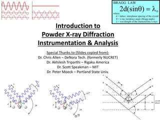
X-ray diffraction is based on constructive interference of monochromatic X-rays and a crystalline sample.
The interaction of the incident rays with the sample produces constructive interference (and a diffracted ray) when conditions satisfy Bragg's Law (nλ=2d sin θ).
XRD Techniques
XRD Techniques
Applications of XRD
Limitations of XRD
XRF
X-Ray Fluorescence is defined as “The emission of characteristic "secondary" (or fluorescent) X-rays from a material that has been excited by bombarding with high-energy X-rays. The phenomenon is widely used for elemental analysis.”
X-ray fluorescence procedures
applied to the material
in any physical state,
solid, liquid and gas.
Principles of XRF
The XRF method depends on fundamental principles that are common to several other instrumental methods involving interactions between electron beams and X-rays with samples, including, X-ray spectroscopy (e.g. SEM – EDS), X-ray diffraction (XRD) and wavelength dispersive spectroscopy (microprobe WDS).
XRF Techniques
Applications of XRF
Advantages of XRF
Limitation of XRF
0
References
1. Elements of physical chemistry by S Glasstone
2. Atkins physical chemistry
3. Pharmaceutical chemistry by LG Chattem
4. Brady, John B., and Boardman, Shelby J., 1995, Introducing Mineralogy Students to X-ray Diffraction Through Optical Diffraction Experiments Using Lasers. Jour. Geol. Education, v. 43 #5, 471-476.
5. Brady, John B., Newton, Robert M., and Boardman, Shelby J., 1995, New Uses for Powder X-ray Diffraction Experiments in the Undergraduate Curriculum. Jour. Geol. Education, v. 43 #5, 466-470.
6. Buhrke, V. E., Jenkins, R., Smith, D. K., A Practical Guide for the Preparation of Specimens for XRF and XRD Analysis, Wiley, 1998.
Comparing Olympus X-Ray Diffraction to conventional XRDOlympus IMS
More information on Olympus XRF and XRD solutions: http://bit.ly/1pZ3zBo
In this presentation we show the benefits and differences between X-Ray Diffraction and conventional XRD.
Our X-ray Fluorescence (XRF) and X-ray Diffraction (XRD) Analyzers provide qualitative and quantitative material characterization for detection, identification, analysis, quality control, process control, regulatory compliance, and screening, for metals and alloys, mining and geology, scrap and recycling, environmental and consumer safety, education and research, and general manufacturing.
To request more information or for a quote, contact us: http://bit.ly/1wh9SWM
Sign up for our newsletter: http://bit.ly/1j5FOTy
CHARACTERIZATION OF CRYSTALLINE AND PARTIALLY CRYSTALLINE SOLIDS BY X-RAY POWDER DIFFRACTION (XRPD)
USP <941>
Every crystalline phase of a given substance produces a characteristic X-ray diffraction pattern.
Diffraction patterns can be obtained from a randomly oriented crystalline powder composed of crystallites (crystalline regions within a particle) or crystal fragments of finite size.
Essentially three types of information can be derived from a powder diffraction pattern:
The angular position of diffraction lines (depending on geometry and size of the unit cell).
The intensities of diffraction lines (depending mainly on atom type and arrangement and preferred orientation within the sample.
Diffraction line profiles (depending on instrumental resolution, crystallite size, strain, and specimen thickness).
X-Ray Diffraction head points:
Introduction
History
How Diffraction Works
Demonstration
Analyzing Diffraction Patterns
Solving DNA
Applications
Summary and Conclusions
https://www.linkedin.com/in/preeti-choudhary-266414182/
https://www.instagram.com/chaudharypreeti1997/
https://www.facebook.com/profile.php?id=100013419194533
https://twitter.com/preetic27018281
Please like, share, comment and follow.
stay connected
If any query then contact:
chaudharypreeti1997@gmail.com
Thanking-You
Preeti Choudhary
What is greenhouse gasses and how many gasses are there to affect the Earth.moosaasad1975
What are greenhouse gasses how they affect the earth and its environment what is the future of the environment and earth how the weather and the climate effects.
THE IMPORTANCE OF MARTIAN ATMOSPHERE SAMPLE RETURN.Sérgio Sacani
The return of a sample of near-surface atmosphere from Mars would facilitate answers to several first-order science questions surrounding the formation and evolution of the planet. One of the important aspects of terrestrial planet formation in general is the role that primary atmospheres played in influencing the chemistry and structure of the planets and their antecedents. Studies of the martian atmosphere can be used to investigate the role of a primary atmosphere in its history. Atmosphere samples would also inform our understanding of the near-surface chemistry of the planet, and ultimately the prospects for life. High-precision isotopic analyses of constituent gases are needed to address these questions, requiring that the analyses are made on returned samples rather than in situ.
Observation of Io’s Resurfacing via Plume Deposition Using Ground-based Adapt...Sérgio Sacani
Since volcanic activity was first discovered on Io from Voyager images in 1979, changes
on Io’s surface have been monitored from both spacecraft and ground-based telescopes.
Here, we present the highest spatial resolution images of Io ever obtained from a groundbased telescope. These images, acquired by the SHARK-VIS instrument on the Large
Binocular Telescope, show evidence of a major resurfacing event on Io’s trailing hemisphere. When compared to the most recent spacecraft images, the SHARK-VIS images
show that a plume deposit from a powerful eruption at Pillan Patera has covered part
of the long-lived Pele plume deposit. Although this type of resurfacing event may be common on Io, few have been detected due to the rarity of spacecraft visits and the previously low spatial resolution available from Earth-based telescopes. The SHARK-VIS instrument ushers in a new era of high resolution imaging of Io’s surface using adaptive
optics at visible wavelengths.
Cancer cell metabolism: special Reference to Lactate PathwayAADYARAJPANDEY1
Normal Cell Metabolism:
Cellular respiration describes the series of steps that cells use to break down sugar and other chemicals to get the energy we need to function.
Energy is stored in the bonds of glucose and when glucose is broken down, much of that energy is released.
Cell utilize energy in the form of ATP.
The first step of respiration is called glycolysis. In a series of steps, glycolysis breaks glucose into two smaller molecules - a chemical called pyruvate. A small amount of ATP is formed during this process.
Most healthy cells continue the breakdown in a second process, called the Kreb's cycle. The Kreb's cycle allows cells to “burn” the pyruvates made in glycolysis to get more ATP.
The last step in the breakdown of glucose is called oxidative phosphorylation (Ox-Phos).
It takes place in specialized cell structures called mitochondria. This process produces a large amount of ATP. Importantly, cells need oxygen to complete oxidative phosphorylation.
If a cell completes only glycolysis, only 2 molecules of ATP are made per glucose. However, if the cell completes the entire respiration process (glycolysis - Kreb's - oxidative phosphorylation), about 36 molecules of ATP are created, giving it much more energy to use.
IN CANCER CELL:
Unlike healthy cells that "burn" the entire molecule of sugar to capture a large amount of energy as ATP, cancer cells are wasteful.
Cancer cells only partially break down sugar molecules. They overuse the first step of respiration, glycolysis. They frequently do not complete the second step, oxidative phosphorylation.
This results in only 2 molecules of ATP per each glucose molecule instead of the 36 or so ATPs healthy cells gain. As a result, cancer cells need to use a lot more sugar molecules to get enough energy to survive.
introduction to WARBERG PHENOMENA:
WARBURG EFFECT Usually, cancer cells are highly glycolytic (glucose addiction) and take up more glucose than do normal cells from outside.
Otto Heinrich Warburg (; 8 October 1883 – 1 August 1970) In 1931 was awarded the Nobel Prize in Physiology for his "discovery of the nature and mode of action of the respiratory enzyme.
WARNBURG EFFECT : cancer cells under aerobic (well-oxygenated) conditions to metabolize glucose to lactate (aerobic glycolysis) is known as the Warburg effect. Warburg made the observation that tumor slices consume glucose and secrete lactate at a higher rate than normal tissues.
Earliest Galaxies in the JADES Origins Field: Luminosity Function and Cosmic ...Sérgio Sacani
We characterize the earliest galaxy population in the JADES Origins Field (JOF), the deepest
imaging field observed with JWST. We make use of the ancillary Hubble optical images (5 filters
spanning 0.4−0.9µm) and novel JWST images with 14 filters spanning 0.8−5µm, including 7 mediumband filters, and reaching total exposure times of up to 46 hours per filter. We combine all our data
at > 2.3µm to construct an ultradeep image, reaching as deep as ≈ 31.4 AB mag in the stack and
30.3-31.0 AB mag (5σ, r = 0.1” circular aperture) in individual filters. We measure photometric
redshifts and use robust selection criteria to identify a sample of eight galaxy candidates at redshifts
z = 11.5 − 15. These objects show compact half-light radii of R1/2 ∼ 50 − 200pc, stellar masses of
M⋆ ∼ 107−108M⊙, and star-formation rates of SFR ∼ 0.1−1 M⊙ yr−1
. Our search finds no candidates
at 15 < z < 20, placing upper limits at these redshifts. We develop a forward modeling approach to
infer the properties of the evolving luminosity function without binning in redshift or luminosity that
marginalizes over the photometric redshift uncertainty of our candidate galaxies and incorporates the
impact of non-detections. We find a z = 12 luminosity function in good agreement with prior results,
and that the luminosity function normalization and UV luminosity density decline by a factor of ∼ 2.5
from z = 12 to z = 14. We discuss the possible implications of our results in the context of theoretical
models for evolution of the dark matter halo mass function.
Slide 1: Title Slide
Extrachromosomal Inheritance
Slide 2: Introduction to Extrachromosomal Inheritance
Definition: Extrachromosomal inheritance refers to the transmission of genetic material that is not found within the nucleus.
Key Components: Involves genes located in mitochondria, chloroplasts, and plasmids.
Slide 3: Mitochondrial Inheritance
Mitochondria: Organelles responsible for energy production.
Mitochondrial DNA (mtDNA): Circular DNA molecule found in mitochondria.
Inheritance Pattern: Maternally inherited, meaning it is passed from mothers to all their offspring.
Diseases: Examples include Leber’s hereditary optic neuropathy (LHON) and mitochondrial myopathy.
Slide 4: Chloroplast Inheritance
Chloroplasts: Organelles responsible for photosynthesis in plants.
Chloroplast DNA (cpDNA): Circular DNA molecule found in chloroplasts.
Inheritance Pattern: Often maternally inherited in most plants, but can vary in some species.
Examples: Variegation in plants, where leaf color patterns are determined by chloroplast DNA.
Slide 5: Plasmid Inheritance
Plasmids: Small, circular DNA molecules found in bacteria and some eukaryotes.
Features: Can carry antibiotic resistance genes and can be transferred between cells through processes like conjugation.
Significance: Important in biotechnology for gene cloning and genetic engineering.
Slide 6: Mechanisms of Extrachromosomal Inheritance
Non-Mendelian Patterns: Do not follow Mendel’s laws of inheritance.
Cytoplasmic Segregation: During cell division, organelles like mitochondria and chloroplasts are randomly distributed to daughter cells.
Heteroplasmy: Presence of more than one type of organellar genome within a cell, leading to variation in expression.
Slide 7: Examples of Extrachromosomal Inheritance
Four O’clock Plant (Mirabilis jalapa): Shows variegated leaves due to different cpDNA in leaf cells.
Petite Mutants in Yeast: Result from mutations in mitochondrial DNA affecting respiration.
Slide 8: Importance of Extrachromosomal Inheritance
Evolution: Provides insight into the evolution of eukaryotic cells.
Medicine: Understanding mitochondrial inheritance helps in diagnosing and treating mitochondrial diseases.
Agriculture: Chloroplast inheritance can be used in plant breeding and genetic modification.
Slide 9: Recent Research and Advances
Gene Editing: Techniques like CRISPR-Cas9 are being used to edit mitochondrial and chloroplast DNA.
Therapies: Development of mitochondrial replacement therapy (MRT) for preventing mitochondrial diseases.
Slide 10: Conclusion
Summary: Extrachromosomal inheritance involves the transmission of genetic material outside the nucleus and plays a crucial role in genetics, medicine, and biotechnology.
Future Directions: Continued research and technological advancements hold promise for new treatments and applications.
Slide 11: Questions and Discussion
Invite Audience: Open the floor for any questions or further discussion on the topic.
A brief information about the SCOP protein database used in bioinformatics.
The Structural Classification of Proteins (SCOP) database is a comprehensive and authoritative resource for the structural and evolutionary relationships of proteins. It provides a detailed and curated classification of protein structures, grouping them into families, superfamilies, and folds based on their structural and sequence similarities.
Comparing Evolved Extractive Text Summary Scores of Bidirectional Encoder Rep...University of Maribor
Slides from:
11th International Conference on Electrical, Electronics and Computer Engineering (IcETRAN), Niš, 3-6 June 2024
Track: Artificial Intelligence
https://www.etran.rs/2024/en/home-english/
Nutraceutical market, scope and growth: Herbal drug technologyLokesh Patil
As consumer awareness of health and wellness rises, the nutraceutical market—which includes goods like functional meals, drinks, and dietary supplements that provide health advantages beyond basic nutrition—is growing significantly. As healthcare expenses rise, the population ages, and people want natural and preventative health solutions more and more, this industry is increasing quickly. Further driving market expansion are product formulation innovations and the use of cutting-edge technology for customized nutrition. With its worldwide reach, the nutraceutical industry is expected to keep growing and provide significant chances for research and investment in a number of categories, including vitamins, minerals, probiotics, and herbal supplements.
Nutraceutical market, scope and growth: Herbal drug technology
Xrd nanomaterials course_s2015_bates
1. Introduction to
Powder X-ray Diffraction
Instrumentation & Analysis
Special Thanks to (Slides copied from):
Dr. Chris Allen – DeNora Tech. (formerly NUCRET)
Dr. Akhilesh Triparthi – Rigaku America
Dr. Scott Speakman – MIT
Dr. Peter Moeck – Portland State Univ.
2. What is Diffraction?
• Traditionally, diffraction refers to the splitting of
polychromatic light into separate wavelengths
**Using a diffraction grating with well-defined ridges
or “gratings” to separate the photons
3. X-ray Diffraction
• XRD uses:
monochromatic light source
so the incident beam isn’t split
into component wavelengths –
there’s only 1 wavelength to
begin with.
• Instead, for XRD we don’t
know the spacing distance of
the diffraction gratings
• XRD can only be used for
samples with periodic
structure (crystals)
• The crystal lattice planes act as
diffraction gratings
No grating,
Just powder sample
Unknown:
“grating length”
Crystal planes
Are the
Diffraction
Grating
6. Other Types of XRD
• More-complex, multi-angle
goniometers are used to study
protein crystal structure
7. XRD & Nanomaterials
• Aside from identification of crystal phase
– (i.e. “fingerprinting” like MS for molecular samples)
• XRD can identify crystallite size & strain
• Size & Strain affect physical properties such as:
– Band-gap for semi-conductors
– Magnetic properties of magnetic materials
• Strain effects can determine the “degree of alloying”
– i.e. quantitative composition of eutectic mixtures of solids
13. 10 20 30 40
2
Atomic
distribution in
the unit cell
Peak relative
intensities
Unit cell
Symmetry
and size
Peak
positions
a
c
b
Peak shapes
Particle size
and defects
Background
Diffuse scattering,
sample holder,
matrix, amorphous
phases, etc...
X-ray Powder Diffraction
51. Rietveld method
•Structural Refinement, not structure solution!!!!
2
Intensity 2
)( cii
i
iy yywS
•Good starting model is a must, since many bragg reflections will
exist at any chosen point of intensity (yi)
Minimize the residual-
•Hugo Rietveld (1960’s)- uncovered that a
modeled pattern could be fit to experimental
data if instrumental and specimen features are
subtracted.
wi-=1/yi
yi= intensity at each step i
yci= calculated intensity
at each step i.
52. Rietveld method
•Structural Refinement, not structure solution!!!!
2
Intensity 2
)( cii
i
iy yywS
•Good starting model is a must, since many bragg reflections will
exist at any chosen point of intensity (yi)
Minimize the residual-
•Hugo Rietveld (1960’s)- uncovered that a
modeled pattern could be fit to experimental
data if instrumental and specimen features are
subtracted.
wi-=1/yi
yi= intensity at each step i
yci= calculated intensity
at each step i.
53. What factors contribute to your calculated intensity (yci)??
biKKiK
K
Kci yAPFLsy )22()( 2
φ= approximates instrumental and specimen features
Instrument
Peak shape asymmetry
Sample
displacement
Transparency
Specimen caused broadening
PK- preferred orientation (orientation of certain crystal faces parallel to sample holder)
Ybi= operator selected points to construct background
A- sample absorption
s- scale factor ( quantitative phase analysis)
LK- Lorentz, polarization, and multiplicity factors (2theta dependent intensities)
FK- structure factor for K bragg reflection
54. Rietveld method
Icalc = Ibck + S Shkl Chkl () F2
hkl () Phkl()
background
Scale
factor Corrections
Miller
Structure
factor
Profile
function
Structure
Symmetry
Experimental
Geometry set-
up
Atomic positions,
site occupancy
& thermal factors
particle size, stress-
strain, texture
+
Experimental
resolution
56. Variables involved in the fit
• Similar to single crystal but experimental
effects must also be included now
» Background
» Peak shape
» Systematic errors (e.g. axial divergence, sample
displacement)
• Sample dependent terms
» Phase fractions (scale factor)
» Structural parameters (atomic positions, thermal
variables)
» Lattice constants
57. Helpful resources for XRD, software & tutorials.
www.aps.anl.gov/Xray_Science_Division/Powder_Diffraction_Crystallography/
Argonne National Laboratory
-GSAS, Expgui/ free downloads + tutorials
-XRD course (Professor Cora Lind)
“The Rietveld Method” R.A. Young (1995)
58. 59
Diffraction with Grazing Incidence
Usually in the case of “thin” films (1 nm~1000 nm) using routine wide
angle X-ray scattering (WAXS, θ/θ mode of data collection) we observe:
Weak signals from the film
Intense signals from the substrate
To avoid intense signal from the substrate and get stronger signal from
the film we can alternatively perform:
Thin film scan (2θ scan with fixed grazing angle of incidence, θ): GIXRD
1. Generally the lower the grazing angle the shallower is the
penetration of the beam is
59. 60
“Thin film scan” (2 scan with fixed )
Thin film
= incidence angle
Substrate
2
Detector
Normal of diffracting lattice planes
Thin film scan (2θ scan with fixed θ)
61. Estimating Crystallite Size
Using XRD
Scott A Speakman, Ph.D.
13-4009A
speakman@mit.edu
http://prism.mit.edu/xray
MIT Center for Materials Science and Engineering
62. Center for Materials Science and Engineering
http://prism.mit.edu/xray
A Brief History of XRD
• 1895- Röntgen publishes the discovery of X-rays
• 1912- Laue observes diffraction of X-rays from a crystal
• when did Scherrer use X-rays to estimate the
crystallite size of nanophase materials?
Scherrer published on the use of XRD to estimate crystallite size in 1918,
a mere 6 years after the first X-ray diffraction pattern was ever observed.
Remember– nanophase science is not quite as new or novel as we like to think.
63. Center for Materials Science and Engineering
http://prism.mit.edu/xray
The Scherrer Equation was published in 1918
• Peak width (B) is inversely proportional to crystallite size (L)
• P. Scherrer, “Bestimmung der Grösse und der inneren Struktur von
Kolloidteilchen mittels Röntgenstrahlen,” Nachr. Ges. Wiss. Göttingen 26
(1918) pp 98-100.
• J.I. Langford and A.J.C. Wilson, “Scherrer after Sixty Years: A Survey and
Some New Results in the Determination of Crystallite Size,” J. Appl. Cryst.
11 (1978) pp 102-113.
( )
cos
2
L
K
B
64. Center for Materials Science and Engineering
http://prism.mit.edu/xray
Which of these diffraction patterns comes from a
nanocrystalline material?
66 67 68 69 70 71 72 73 74
2(deg.)
Intensity(a.u.)
• These diffraction patterns were produced from the exact same sample
• Two different diffractometers, with different optical configurations, were used
• The apparent peak broadening is due solely to the instrumentation
65. Center for Materials Science and Engineering
http://prism.mit.edu/xray
Many factors may contribute to
the observed peak profile
• Instrumental Peak Profile
• Crystallite Size
• Microstrain
– Non-uniform Lattice Distortions
– Faulting
– Dislocations
– Antiphase Domain Boundaries
– Grain Surface Relaxation
• Solid Solution Inhomogeneity
• Temperature Factors
• The peak profile is a convolution of the profiles from all of
these contributions
66. Center for Materials Science and Engineering
http://prism.mit.edu/xray
Instrument and Sample Contributions to the Peak
Profile must be Deconvoluted
• In order to analyze crystallite size, we must deconvolute:
– Instrumental Broadening FW(I)
• also referred to as the Instrumental Profile, Instrumental
FWHM Curve, Instrumental Peak Profile
– Specimen Broadening FW(S)
• also referred to as the Sample Profile, Specimen Profile
• We must then separate the different contributions to
specimen broadening
– Crystallite size and microstrain broadening of diffraction peaks
67. Center for Materials Science and Engineering
http://prism.mit.edu/xray
Contributions to Peak Profile
1. Peak broadening due to crystallite size
2. Peak broadening due to the instrumental profile
3. Which instrument to use for nanophase analysis
4. Peak broadening due to microstrain
• the different types of microstrain
• Peak broadening due to solid solution inhomogeneity
and due to temperature factors
68. Center for Materials Science and Engineering
http://prism.mit.edu/xray
Crystallite Size Broadening
• Peak Width due to crystallite size varies inversely with crystallite
size
– as the crystallite size gets smaller, the peak gets broader
• The peak width varies with 2 as cos
– The crystallite size broadening is most pronounced at large angles
2Theta
• However, the instrumental profile width and microstrain
broadening are also largest at large angles 2theta
• peak intensity is usually weakest at larger angles 2theta
– If using a single peak, often get better results from using diffraction
peaks between 30 and 50 deg 2theta
• below 30deg 2theta, peak asymmetry compromises profile
analysis
( )
cos
2
L
K
B
69. Center for Materials Science and Engineering
http://prism.mit.edu/xray
The Scherrer Constant, K
• The constant of proportionality, K (the Scherrer constant)
depends on the how the width is determined, the shape of the
crystal, and the size distribution
– the most common values for K are:
• 0.94 for FWHM of spherical crystals with cubic symmetry
• 0.89 for integral breadth of spherical crystals w/ cubic symmetry
• 1, because 0.94 and 0.89 both round up to 1
– K actually varies from 0.62 to 2.08
• For an excellent discussion of K, refer to JI Langford and AJC
Wilson, “Scherrer after sixty years: A survey and some new
results in the determination of crystallite size,” J. Appl. Cryst. 11
(1978) p102-113.
( )
cos
2
L
K
B ( )
cos
94.0
2
L
B
70. Center for Materials Science and Engineering
http://prism.mit.edu/xray
Factors that affect K and crystallite size analysis
• how the peak width is defined
• how crystallite size is defined
• the shape of the crystal
• the size distribution
71. Center for Materials Science and Engineering
http://prism.mit.edu/xray
46.7 46.8 46.9 47.0 47.1 47.2 47.3 47.4 47.5 47.6 47.7 47.8 47.9
2 (deg.)
Intensity(a.u.)
Methods used in Jade to Define Peak Width
• Full Width at Half Maximum
(FWHM)
– the width of the diffraction peak,
in radians, at a height half-way
between background and the
peak maximum
• Integral Breadth
– the total area under the peak
divided by the peak height
– the width of a rectangle having
the same area and the same
height as the peak
– requires very careful evaluation
of the tails of the peak and the
background
46.746.846.947.047.147.247.347.447.547.647.747.847.9
2(deg.)
Intensity(a.u.)
FWHM
72. Center for Materials Science and Engineering
http://prism.mit.edu/xray
Integral Breadth
• Warren suggests that the Stokes and Wilson method of
using integral breadths gives an evaluation that is
independent of the distribution in size and shape
– L is a volume average of the crystal thickness in the direction
normal to the reflecting planes
– The Scherrer constant K can be assumed to be 1
• Langford and Wilson suggest that even when using the integral
breadth, there is a Scherrer constant K that varies with the shape of
the crystallites
( )
cos
2
L
73. Center for Materials Science and Engineering
http://prism.mit.edu/xray
Other methods used to determine peak width
• These methods are used in more the variance methods, such as
Warren-Averbach analysis
– Most often used for dislocation and defect density analysis of metals
– Can also be used to determine the crystallite size distribution
– Requires no overlap between neighboring diffraction peaks
• Variance-slope
– the slope of the variance of the line profile as a function of the range of
integration
• Variance-intercept
– negative initial slope of the Fourier transform of the normalized line
profile
74. Center for Materials Science and Engineering
http://prism.mit.edu/xray
How is Crystallite Size Defined
• Usually taken as the cube root of the volume of a crystallite
– assumes that all crystallites have the same size and shape
• For a distribution of sizes, the mean size can be defined as
– the mean value of the cube roots of the individual crystallite volumes
– the cube root of the mean value of the volumes of the individual
crystallites
• Scherrer method (using FWHM) gives the ratio of the root-mean-
fourth-power to the root-mean-square value of the thickness
• Stokes and Wilson method (using integral breadth) determines the
volume average of the thickness of the crystallites measured
perpendicular to the reflecting plane
• The variance methods give the ratio of the total volume of the
crystallites to the total area of their projection on a plane parallel to
the reflecting planes
75. Center for Materials Science and Engineering
http://prism.mit.edu/xray
Remember, Crystallite Size is Different than
Particle Size
• A particle may be made up of several different
crystallites
• Crystallite size often matches grain size, but there are
exceptions
76. Center for Materials Science and Engineering
http://prism.mit.edu/xray
Crystallite Shape
• Though the shape of crystallites is usually irregular, we can often
approximate them as:
– sphere, cube, tetrahedra, or octahedra
– parallelepipeds such as needles or plates
– prisms or cylinders
• Most applications of Scherrer analysis assume spherical crystallite
shapes
• If we know the average crystallite shape from another analysis, we
can select the proper value for the Scherrer constant K
• Anistropic peak shapes can be identified by anistropic peak
broadening
– if the dimensions of a crystallite are 2x * 2y * 200z, then (h00) and (0k0)
peaks will be more broadened then (00l) peaks.
77. Center for Materials Science and Engineering
http://prism.mit.edu/xray
Anistropic Size Broadening
• The broadening of a single diffraction peak is the product of the
crystallite dimensions in the direction perpendicular to the planes
that produced the diffraction peak.
78. Center for Materials Science and Engineering
http://prism.mit.edu/xray
Crystallite Size Distribution
• is the crystallite size narrowly or broadly distributed?
• is the crystallite size unimodal?
• XRD is poorly designed to facilitate the analysis of crystallites with a
broad or multimodal size distribution
• Variance methods, such as Warren-Averbach, can be used to
quantify a unimodal size distribution
– Otherwise, we try to accommodate the size distribution in the Scherrer
constant
– Using integral breadth instead of FWHM may reduce the effect of
crystallite size distribution on the Scherrer constant K and therefore the
crystallite size analysis
79. Center for Materials Science and Engineering
http://prism.mit.edu/xray
Instrumental Peak Profile
• A large crystallite size, defect-free powder
specimen will still produce diffraction
peaks with a finite width
• The peak widths from the instrument peak
profile are a convolution of:
– X-ray Source Profile
• Wavelength widths of Ka1 and Ka2
lines
• Size of the X-ray source
• Superposition of Ka1 and Ka2 peaks
– Goniometer Optics
• Divergence and Receiving Slit widths
• Imperfect focusing
• Beam size
• Penetration into the sample
47.0 47.2 47.4 47.6 47.8
2(deg.)
Intensity(a.u.)
Patterns collected from the same
sample with different instruments
and configurations at MIT
80. Center for Materials Science and Engineering
http://prism.mit.edu/xray
What Instrument to Use?
• The instrumental profile determines the upper limit of crystallite
size that can be evaluated
– if the Instrumental peak width is much larger than the broadening
due to crystallite size, then we cannot accurately determine
crystallite size
– For analyzing larger nanocrystallites, it is important to use the
instrument with the smallest instrumental peak width
• Very small nanocrystallites produce weak signals
– the specimen broadening will be significantly larger than the
instrumental broadening
– the signal:noise ratio is more important than the instrumental
profile
81. Center for Materials Science and Engineering
http://prism.mit.edu/xray
Comparison of Peak Widths at 47° 2 for
Instruments and Crystallite Sizes
• Rigaku XRPD is better for very small nanocrystallites, <80 nm (upper limit 100 nm)
• PANalytical X’Pert Pro is better for larger nanocrystallites, <150 nm
Configuration FWHM
(deg)
Pk Ht to
Bkg
Ratio
Rigaku, LHS, 0.5° DS, 0.3mm RS 0.076 528
Rigaku, LHS, 1° DS, 0.3mm RS 0.097 293
Rigaku, RHS, 0.5° DS, 0.3mm RS 0.124 339
Rigaku, RHS, 1° DS, 0.3mm RS 0.139 266
X’Pert Pro, High-speed, 0.25° DS 0.060 81
X’Pert Pro, High-speed, 0.5° DS 0.077 72
X’Pert, 0.09° Parallel Beam Collimator 0.175 50
X’Pert, 0.27° Parallel Beam Collimator 0.194 55
Crystallite
Size
FWHM
(deg)
100 nm 0.099
50 nm 0.182
10 nm 0.871
5 nm 1.745
82. Center for Materials Science and Engineering
http://prism.mit.edu/xray
Other Instrumental Considerations
for Thin Films
• The irradiated area greatly affects the intensity of
high angle diffraction peaks
– GIXD or variable divergence slits on the
PANalytical X’Pert Pro will maintain a constant
irradiated area, increasing the signal for high angle
diffraction peaks
– both methods increase the instrumental FWHM
• Bragg-Brentano geometry only probes crystallite
dimensions through the thickness of the film
– in order to probe lateral (in-plane) crystallite sizes,
need to collect diffraction patterns at different tilts
– this requires the use of parallel-beam optics on the
PANalytical X’Pert Pro, which have very large
FWHM and poor signal:noise ratios
83. Center for Materials Science and Engineering
http://prism.mit.edu/xray
Microstrain Broadening
• lattice strains from displacements of the unit cells about their
normal positions
• often produced by dislocations, domain boundaries, surfaces etc.
• microstrains are very common in nanocrystalline materials
• the peak broadening due to microstrain will vary as:
( )
cos
sin
42 B
compare to peak broadening due to crystallite size: ( )
cos
2
L
K
B
84. Center for Materials Science and Engineering
http://prism.mit.edu/xray
Contributions to Microstrain Broadening
• Non-uniform Lattice Distortions
• Dislocations
• Antiphase Domain Boundaries
• Grain Surface Relaxation
• Other contributions to broadening
– faulting
– solid solution inhomogeneity
– temperature factors
85. Center for Materials Science and Engineering
http://prism.mit.edu/xray
Non-Uniform Lattice Distortions
• Rather than a single d-spacing,
the crystallographic plane has a
distribution of d-spaces
• This produces a broader
observed diffraction peak
• Such distortions can be
introduced by:
– surface tension of nanocrystals
– morphology of crystal shape, such
as nanotubes
– interstitial impurities
26.5 27.0 27.5 28.0 28.5 29.0 29.5 30.0
2(deg.)
Intensity(a.u.)
86. Center for Materials Science and Engineering
http://prism.mit.edu/xray
Antiphase Domain Boundaries
• Formed during the ordering of a material that goes
through an order-disorder transformation
• The fundamental peaks are not affected
• the superstructure peaks are broadened
– the broadening of superstructure peaks varies with hkl
87. Center for Materials Science and Engineering
http://prism.mit.edu/xray
Dislocations
• Line broadening due to dislocations has a strong hkl
dependence
• The profile is Lorentzian
• Can try to analyze by separating the Lorentzian and
Gaussian components of the peak profile
• Can also determine using the Warren-Averbach method
– measure several orders of a peak
• 001, 002, 003, 004, …
• 110, 220, 330, 440, …
– The Fourier coefficient of the sample broadening will contain
• an order independent term due to size broadening
• an order dependent term due to strain
88. Center for Materials Science and Engineering
http://prism.mit.edu/xray
Faulting
• Broadening due to deformation faulting and twin faulting
will convolute with the particle size Fourier coefficient
– The particle size coefficient determined by Warren-Averbach
analysis actually contains contributions from the crystallite size
and faulting
– the fault contribution is hkl dependent, while the size contribution
should be hkl independent (assuming isotropic crystallite shape)
– the faulting contribution varies as a function of hkl dependent on
the crystal structure of the material (fcc vs bcc vs hcp)
– See Warren, 1969, for methods to separate the contributions
from deformation and twin faulting
89. Center for Materials Science and Engineering
http://prism.mit.edu/xray
CeO2
19 nm
45 46 47 48 49 50 51 52
2(deg.)
Intensity(a.u.)
ZrO2
46nm
CexZr1-xO2
0<x<1
Solid Solution Inhomogeneity
• Variation in the composition of a solid solution can create
a distribution of d-spacing for a crystallographic plane
– Similar to the d-spacing distribution created from microstrain due
to non-uniform lattice distortions
90. Center for Materials Science and Engineering
http://prism.mit.edu/xray
Temperature Factor
• The Debye-Waller temperature factor describes the oscillation of an
atom around its average position in the crystal structure
• The thermal agitation results in intensity from the peak maxima being
redistributed into the peak tails
– it does not broaden the FWHM of the diffraction peak, but it does broaden
the integral breadth of the diffraction peak
• The temperature factor increases with 2Theta
• The temperature factor must be convoluted with the structure factor for
each peak
– different atoms in the crystal may have different temperature factors
– each peak contains a different contribution from the atoms in the crystal
( )MfF exp
2
2 3/
2
d
X
M
91. Center for Materials Science and Engineering
http://prism.mit.edu/xray
Determining the Sample Broadening due to
crystallite size
• The sample profile FW(S) can be deconvoluted from the
instrumental profile FW(I) either numerically or by Fourier transform
• In Jade size and strain analysis
– you individually profile fit every diffraction peak
– deconvolute FW(I) from the peak profile functions to isolate FW(S)
– execute analyses on the peak profile functions rather than on the raw
data
• Jade can also use iterative folding to deconvolute FW(I) from the
entire observed diffraction pattern
– this produces an entire diffraction pattern without an instrumental
contribution to peak widths
– this does not require fitting of individual diffraction peaks
– folding increases the noise in the observed diffraction pattern
• Warren Averbach analyses operate on the Fourier transform of the
diffraction peak
– take Fourier transform of peak profile functions or of raw data
92. Center for Materials Science and Engineering
http://prism.mit.edu/xray
Instrumental FWHM Calibration Curve
• The instrument itself contributes to the peak profile
• Before profile fitting the nanocrystalline phase(s) of
interest
– profile fit a calibration standard to determine the
instrumental profile
• Important factors for producing a calibration curve
– Use the exact same instrumental conditions
• same optical configuration of diffractometer
• same sample preparation geometry
• calibration curve should cover the 2theta range of interest for
the specimen diffraction pattern
– do not extrapolate the calibration curve
93. Center for Materials Science and Engineering
http://prism.mit.edu/xray
Instrumental FWHM Calibration Curve
• Standard should share characteristics with the nanocrystalline
specimen
– similar mass absorption coefficient
– similar atomic weight
– similar packing density
• The standard should not contribute to the diffraction peak profile
– macrocrystalline: crystallite size larger than 500 nm
– particle size less than 10 microns
– defect and strain free
• There are several calibration techniques
– Internal Standard
– External Standard of same composition
– External Standard of different composition
94. Center for Materials Science and Engineering
http://prism.mit.edu/xray
Internal Standard Method for Calibration
• Mix a standard in with your nanocrystalline specimen
• a NIST certified standard is preferred
– use a standard with similar mass absorption coefficient
– NIST 640c Si
– NIST 660a LaB6
– NIST 674b CeO2
– NIST 675 Mica
• standard should have few, and preferably no,
overlapping peaks with the specimen
– overlapping peaks will greatly compromise accuracy of analysis
95. Center for Materials Science and Engineering
http://prism.mit.edu/xray
Internal Standard Method for Calibration
• Advantages:
– know that standard and specimen patterns were collected under
identical circumstances for both instrumental conditions and
sample preparation conditions
– the linear absorption coefficient of the mixture is the same for
standard and specimen
• Disadvantages:
– difficult to avoid overlapping peaks between standard and
broadened peaks from very nanocrystalline materials
– the specimen is contaminated
– only works with a powder specimen
96. Center for Materials Science and Engineering
http://prism.mit.edu/xray
External Standard Method for Calibration
• If internal calibration is not an option, then use external
calibration
• Run calibration standard separately from specimen,
keeping as many parameters identical as is possible
• The best external standard is a macrocrystalline
specimen of the same phase as your nanocrystalline
specimen
– How can you be sure that macrocrystalline specimen does not
contribute to peak broadening?
97. Center for Materials Science and Engineering
http://prism.mit.edu/xray
Qualifying your Macrocrystalline Standard
• select powder for your potential macrocrystalline standard
– if not already done, possibly anneal it to allow crystallites to grow and to
allow defects to heal
• use internal calibration to validate that macrocrystalline specimen is
an appropriate standard
– mix macrocrystalline standard with appropriate NIST SRM
– compare FWHM curves for macrocrystalline specimen and NIST
standard
– if the macrocrystalline FWHM curve is similar to that from the NIST
standard, than the macrocrystalline specimen is suitable
– collect the XRD pattern from pure sample of you macrocrystalline
specimen
• do not use the FHWM curve from the mixture with the NIST SRM
98. Center for Materials Science and Engineering
http://prism.mit.edu/xray
Disadvantages/Advantages of External Calibration with a
Standard of the Same Composition
• Advantages:
– will produce better calibration curve because mass absorption
coefficient, density, molecular weight are the same as your specimen of
interest
– can duplicate a mixture in your nanocrystalline specimen
– might be able to make a macrocrystalline standard for thin film samples
• Disadvantages:
– time consuming
– desire a different calibration standard for every different nanocrystalline
phase and mixture
– macrocrystalline standard may be hard/impossible to produce
– calibration curve will not compensate for discrepancies in instrumental
conditions or sample preparation conditions between the standard and
the specimen
99. Center for Materials Science and Engineering
http://prism.mit.edu/xray
External Standard Method of Calibration using a
NIST standard
• As a last resort, use an external standard of a
composition that is different than your nanocrystalline
specimen
– This is actually the most common method used
– Also the least accurate method
• Use a certified NIST standard to produce instrumental
FWHM calibration curve
100. Center for Materials Science and Engineering
http://prism.mit.edu/xray
Advantages and Disadvantages of using NIST
standard for External Calibration
• Advantages
– only need to build one calibration curve for each instrumental
configuration
– I have NIST standard diffraction patterns for each instrument and
configuration available for download from
http://prism.mit.edu/xray/standards.htm
– know that the standard is high quality if from NIST
– neither standard nor specimen are contaminated
• Disadvantages
– The standard may behave significantly different in diffractometer than
your specimen
• different mass absorption coefficient
• different depth of penetration of X-rays
– NIST standards are expensive
– cannot duplicate exact conditions for thin films
101. Center for Materials Science and Engineering
http://prism.mit.edu/xray
Consider- when is good calibration most essential?
• For a very small crystallite size, the specimen broadening dominates
over instrumental broadening
• Only need the most exacting calibration when the specimen broadening
is small because the specimen is not highly nanocrystalline
FWHM of Instrumental Profile
at 48° 2
0.061 deg
Broadening Due to
Nanocrystalline Size
Crystallite Size B(2)
(rad)
FWHM
(deg)
100 nm 0.0015 0.099
50 nm 0.0029 0.182
10 nm 0.0145 0.871
5 nm 0.0291 1.745
102. Center for Materials Science and Engineering
http://prism.mit.edu/xray
Williamson Hall Plot
( ) ( ) ( )
sin4cos
Strain
Size
K
SFW
y-intercept slope
FW(S)*Cos(Theta)
Sin(Theta)0.000 0.784
0.000
4.244
*Fit Size/Strain: XS(Å) = 33 (1), Strain(%) = 0.805 (0.0343), ESD of Fit = 0.00902, LC = 0.751
103. Center for Materials Science and Engineering
http://prism.mit.edu/xray
Manipulating Options in the
Size-Strain Plot of Jade
1. Select Mode of
Analysis
• Fit Size/Strain
• Fit Size
• Fit Strain
2. Select Instrument
Profile Curve
3. Show Origin
4. Deconvolution
Parameter
5. Results
6. Residuals for
Evaluation of Fit
7. Export or Save
1 2 3 4
5 6
7
104. Center for Materials Science and Engineering
http://prism.mit.edu/xray
Analysis Mode: Fit Size Only
( ) ( ) ( )
sin4cos
Strain
Size
K
SFW
slope= 0= strain
FW(S)*Cos(Theta)
Sin(Theta)0.000 0.784
0.000
4.244
*Fit Size Only: XS(Å) = 26 (1), Strain(%) = 0.0, ESD of Fit = 0.00788, LC = 0.751
105. Center for Materials Science and Engineering
http://prism.mit.edu/xray
Analysis Mode: Fit Strain Only
( ) ( ) ( )
sin4cos
Strain
Size
K
SFW
y-intercept= 0
size= ∞
FW(S)*Cos(Theta)
Sin(Theta)0.000 0.784
0.000
4.244
*Fit Strain Only: XS(Å) = 0, Strain(%) = 3.556 (0.0112), ESD of Fit = 0.03018, LC = 0.751
106. Center for Materials Science and Engineering
http://prism.mit.edu/xray
Analysis Mode: Fit Size/Strain
( ) ( ) ( )
sin4cos
Strain
Size
K
SFWFW(S)*Cos(Theta)
Sin(Theta)0.000 0.784
0.000
4.244
*Fit Size/Strain: XS(Å) = 33 (1), Strain(%) = 0.805 (0.0343), ESD of Fit = 0.00902, LC = 0.751
107. Center for Materials Science and Engineering
http://prism.mit.edu/xray
Comparing Results
Size (A) Strain (%) ESD of
Fit
Size(A) Strain(%) ESD of
Fit
Size
Only
22(1) - 0.0111 25(1) 0.0082
Strain
Only
- 4.03(1) 0.0351 3.56(1) 0.0301
Size &
Strain
28(1) 0.935(35) 0.0125 32(1) 0.799(35) 0.0092
Avg from
Scherrer
Analysis
22.5 25.1
Integral Breadth FWHM