
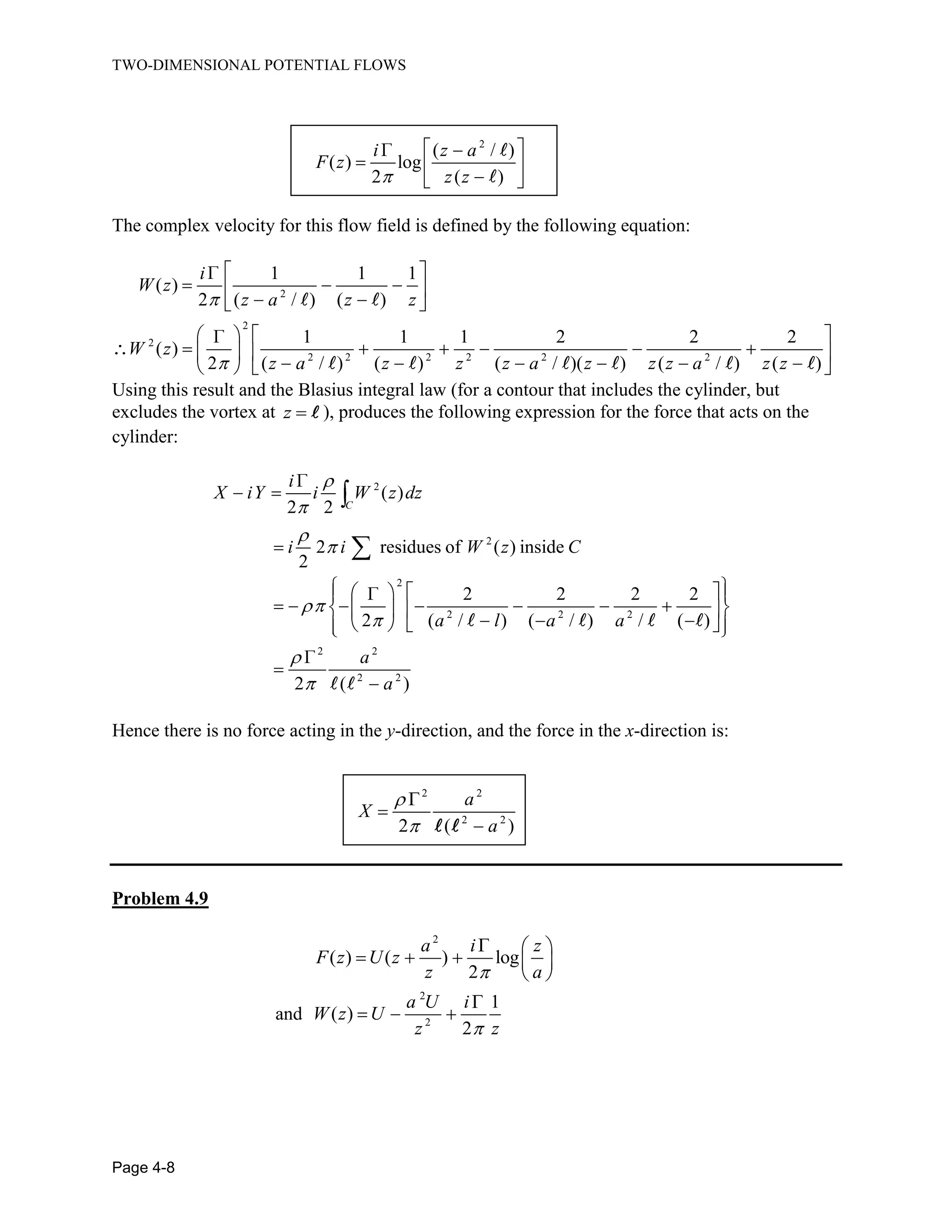
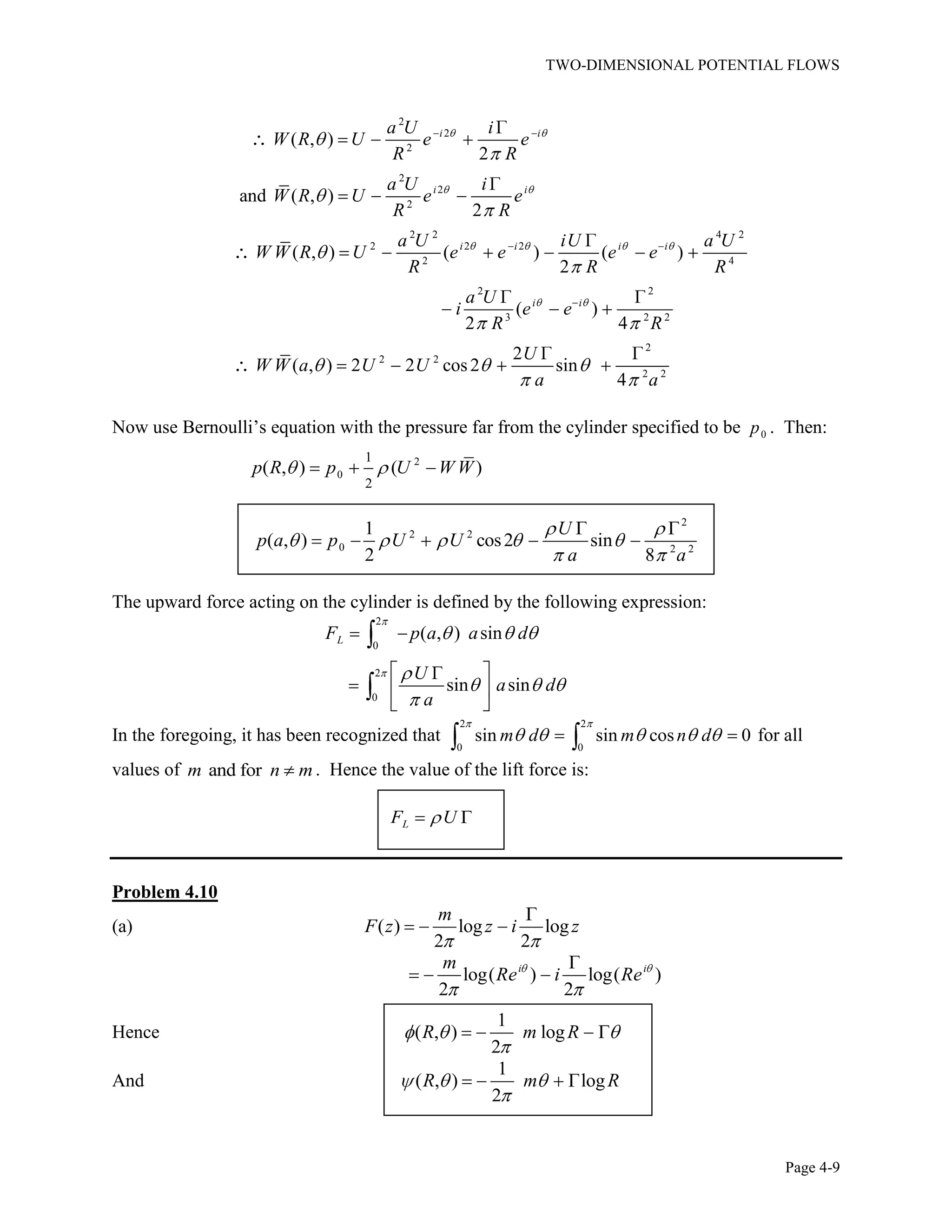
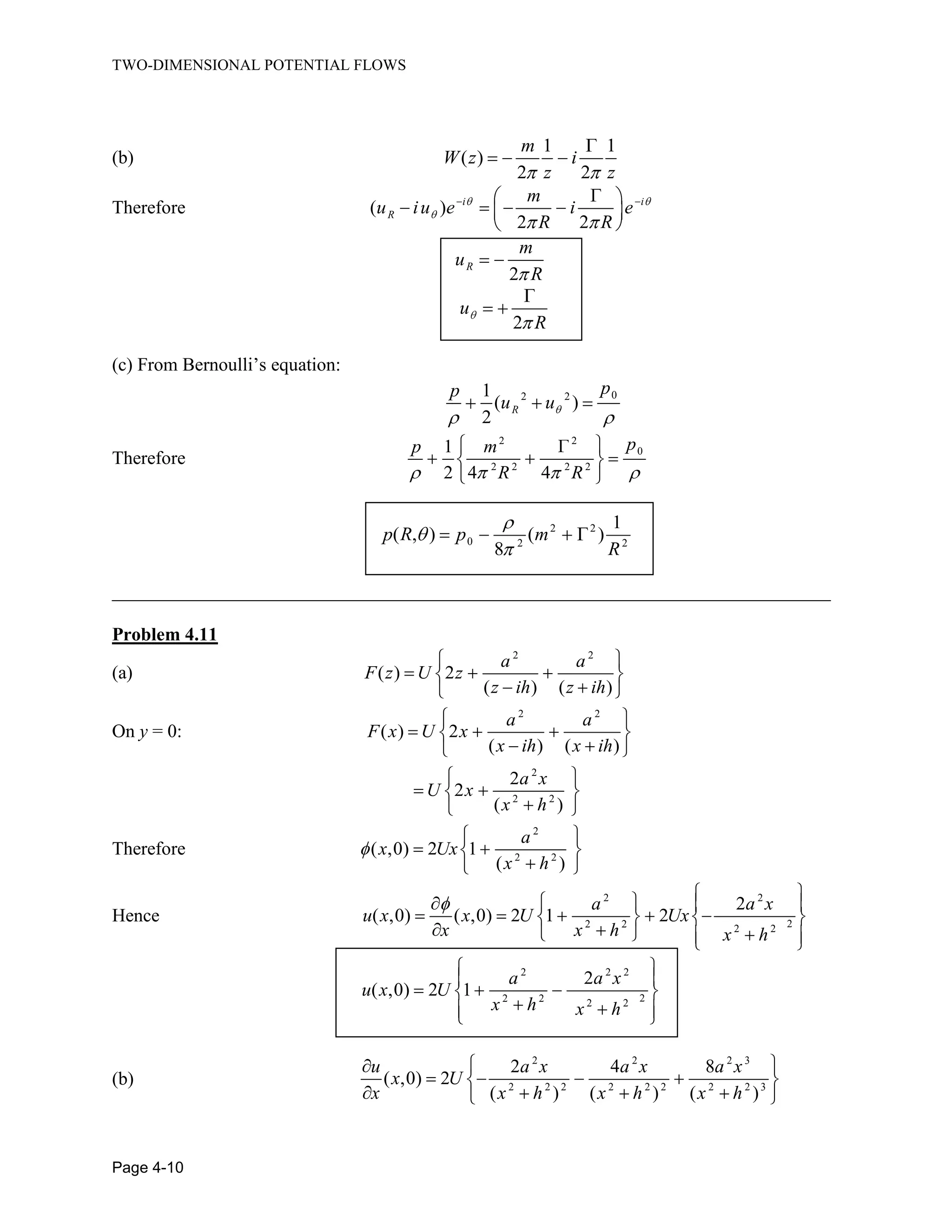
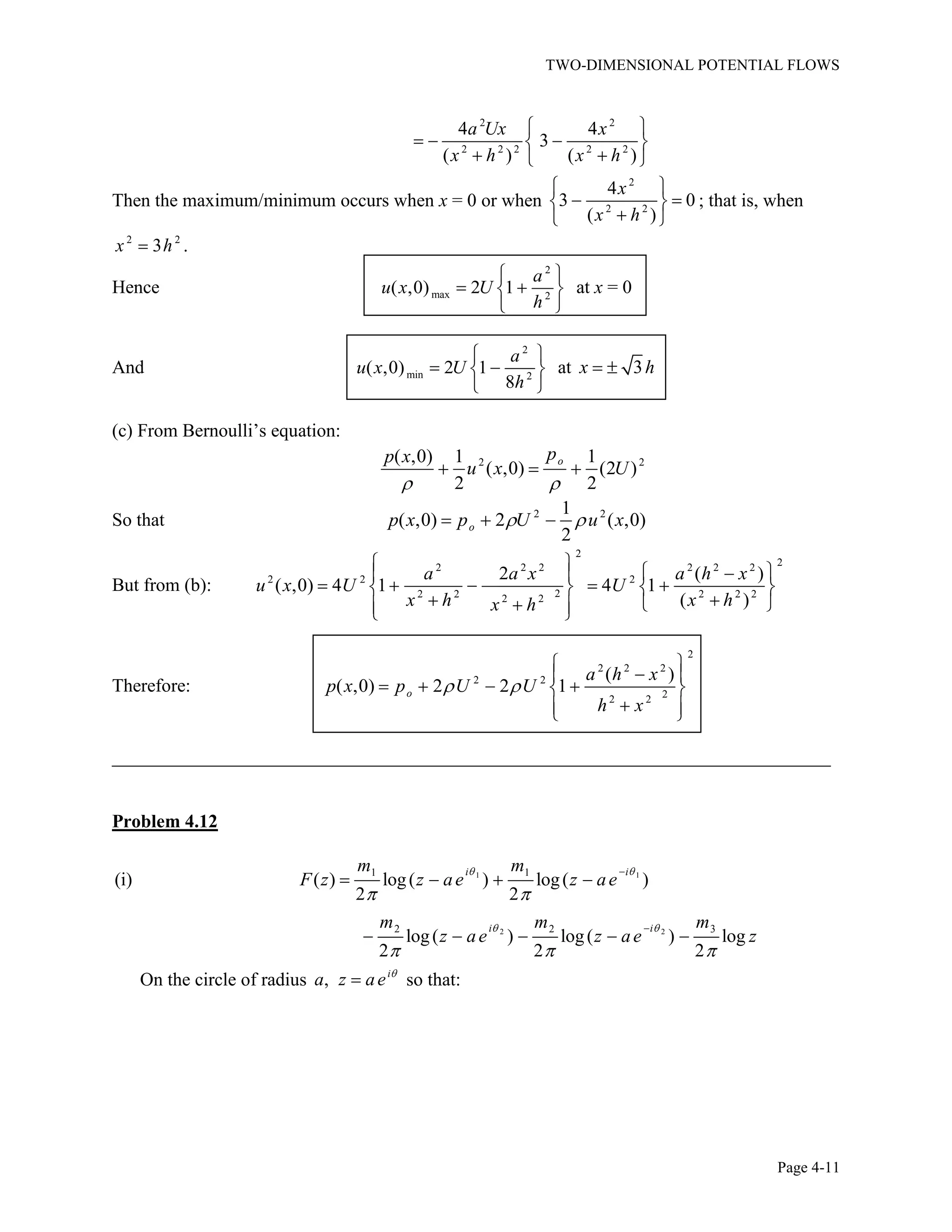
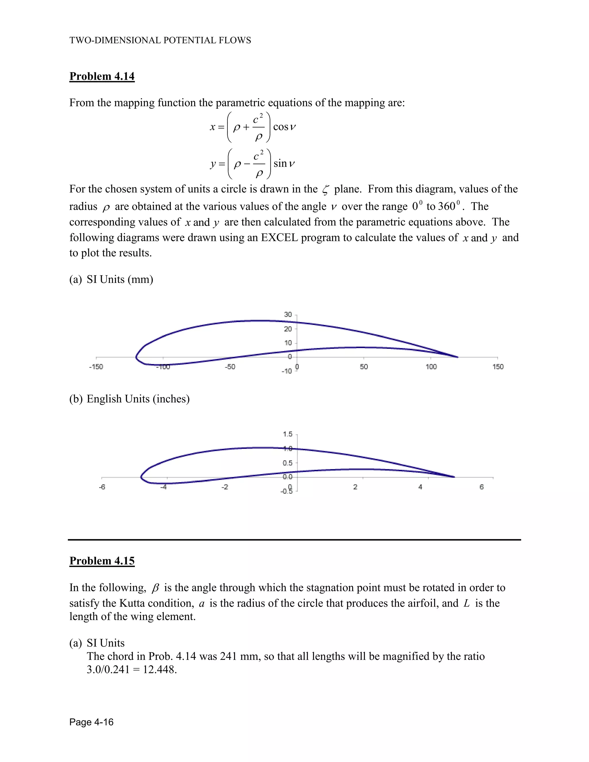
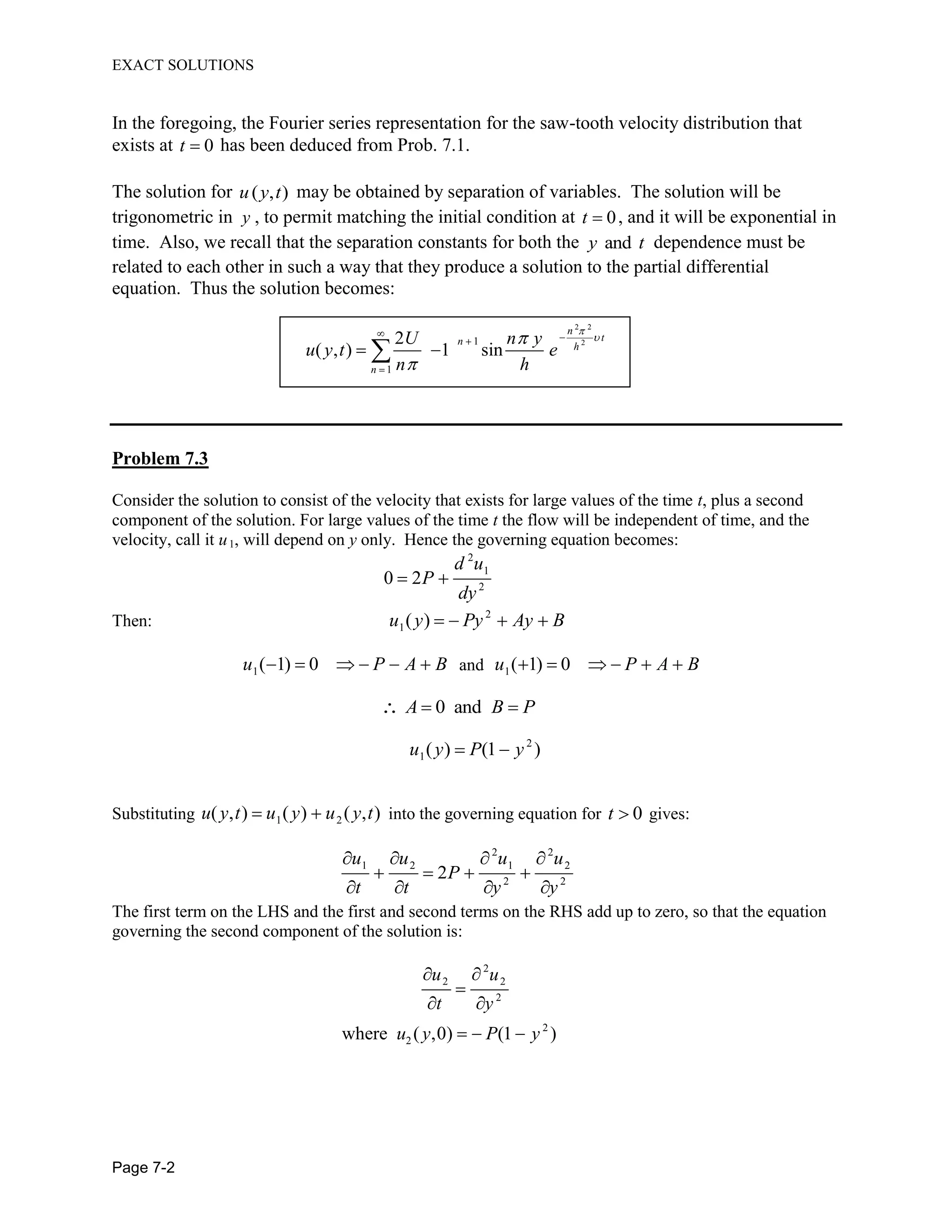
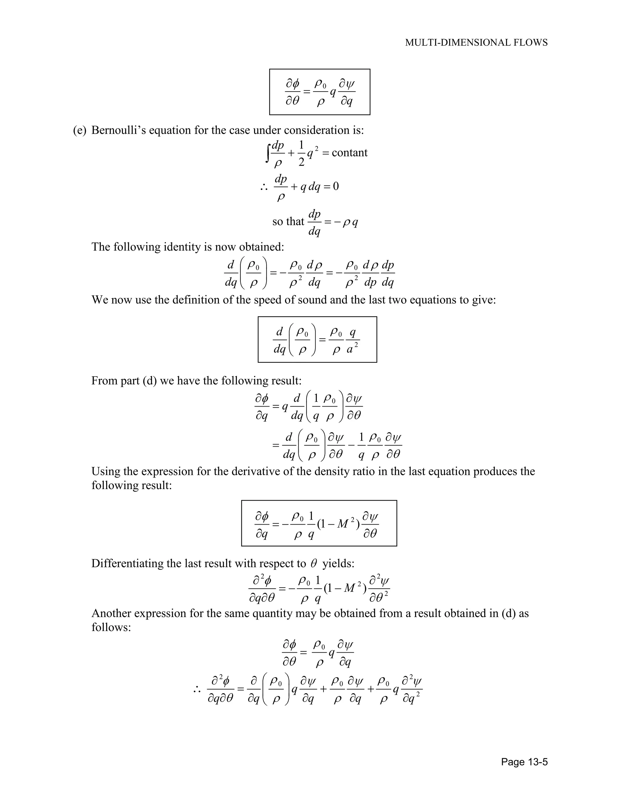
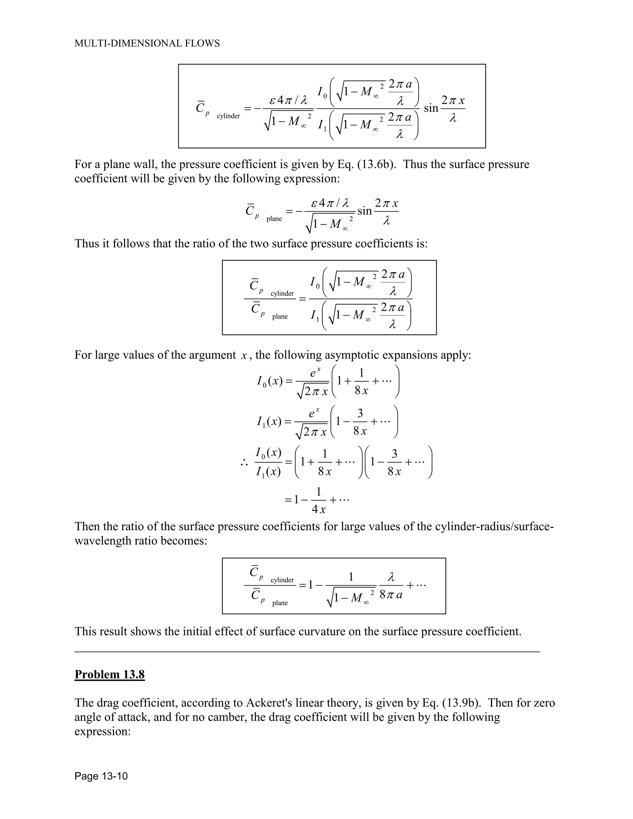
Downloaded 107 times


![BASIC CONSERVATION LAWS
Page 1-4
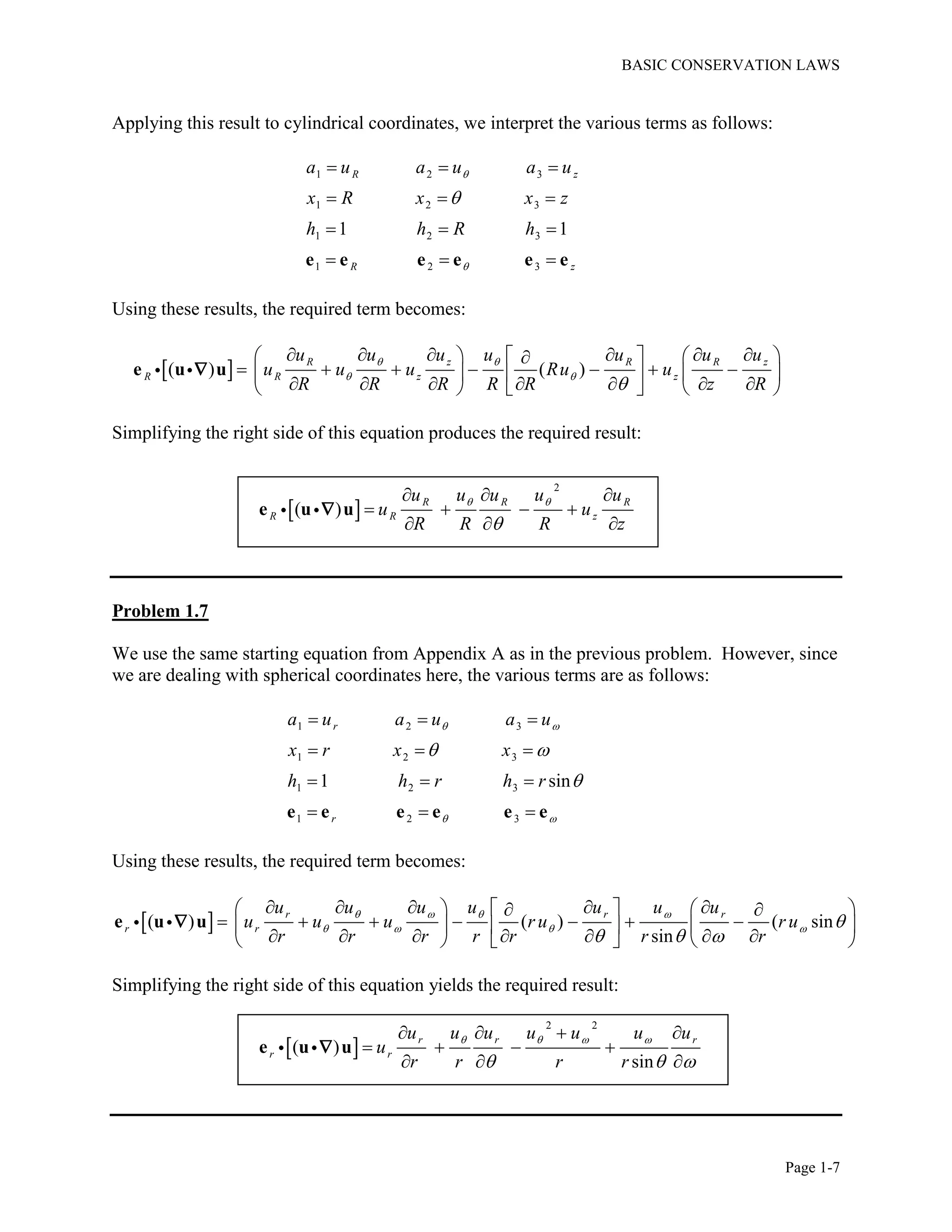
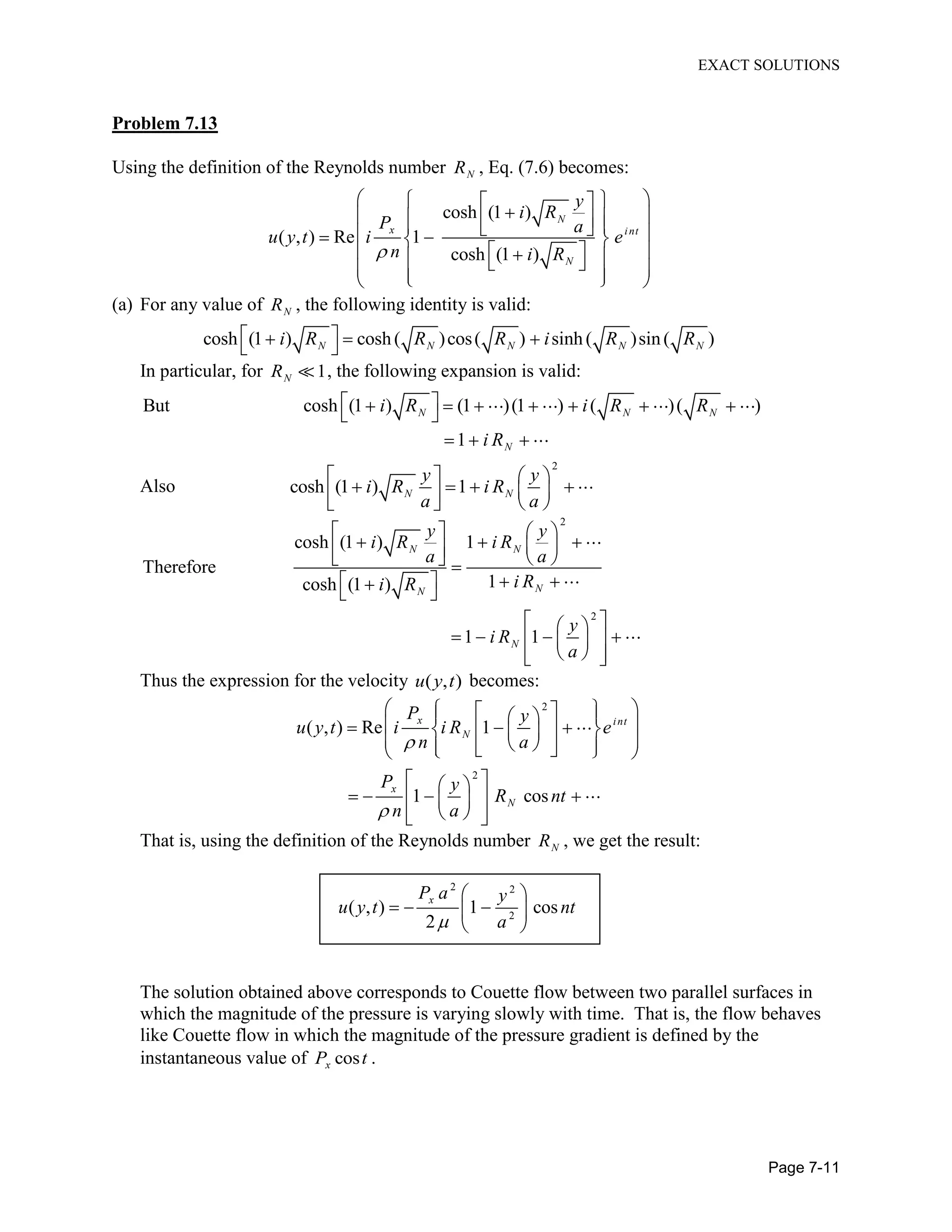
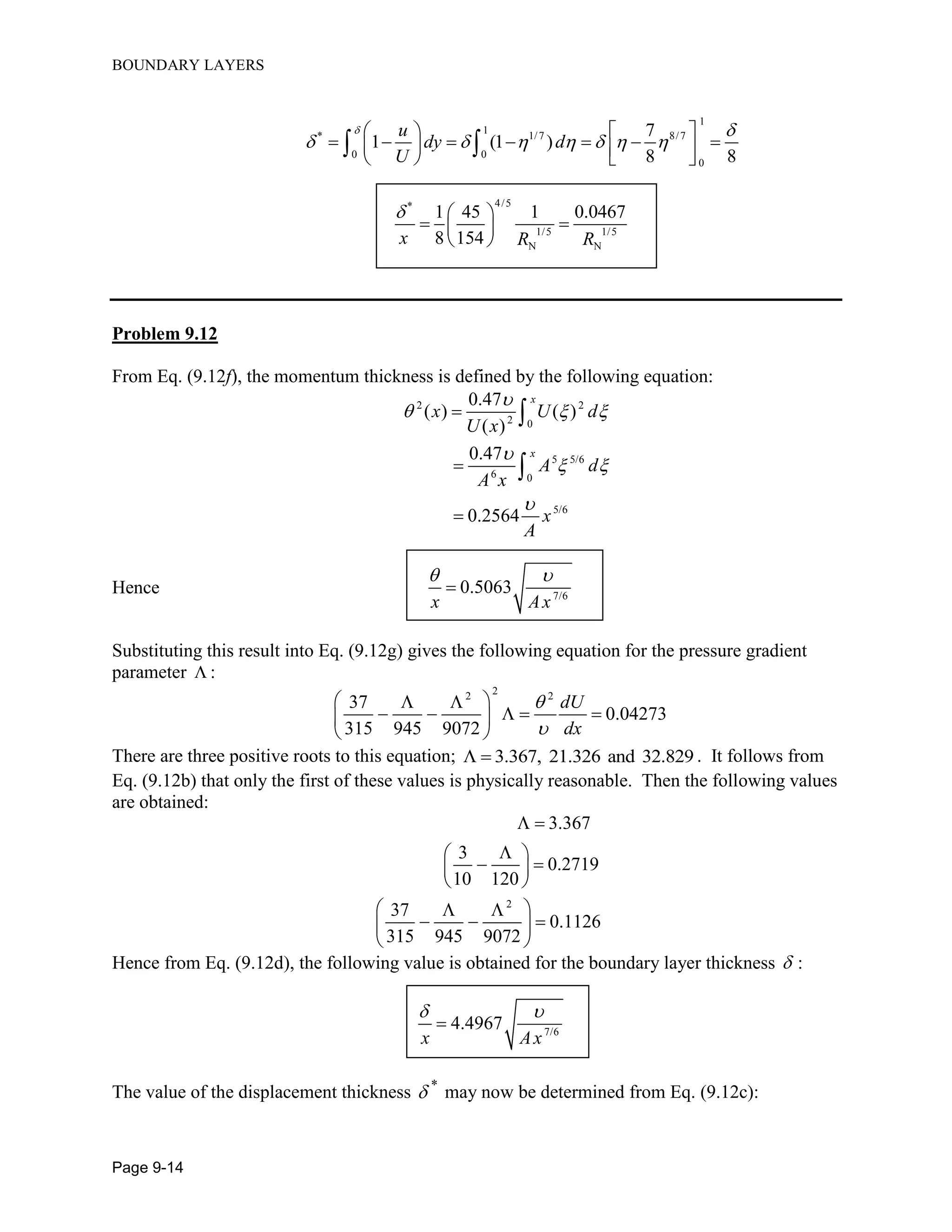
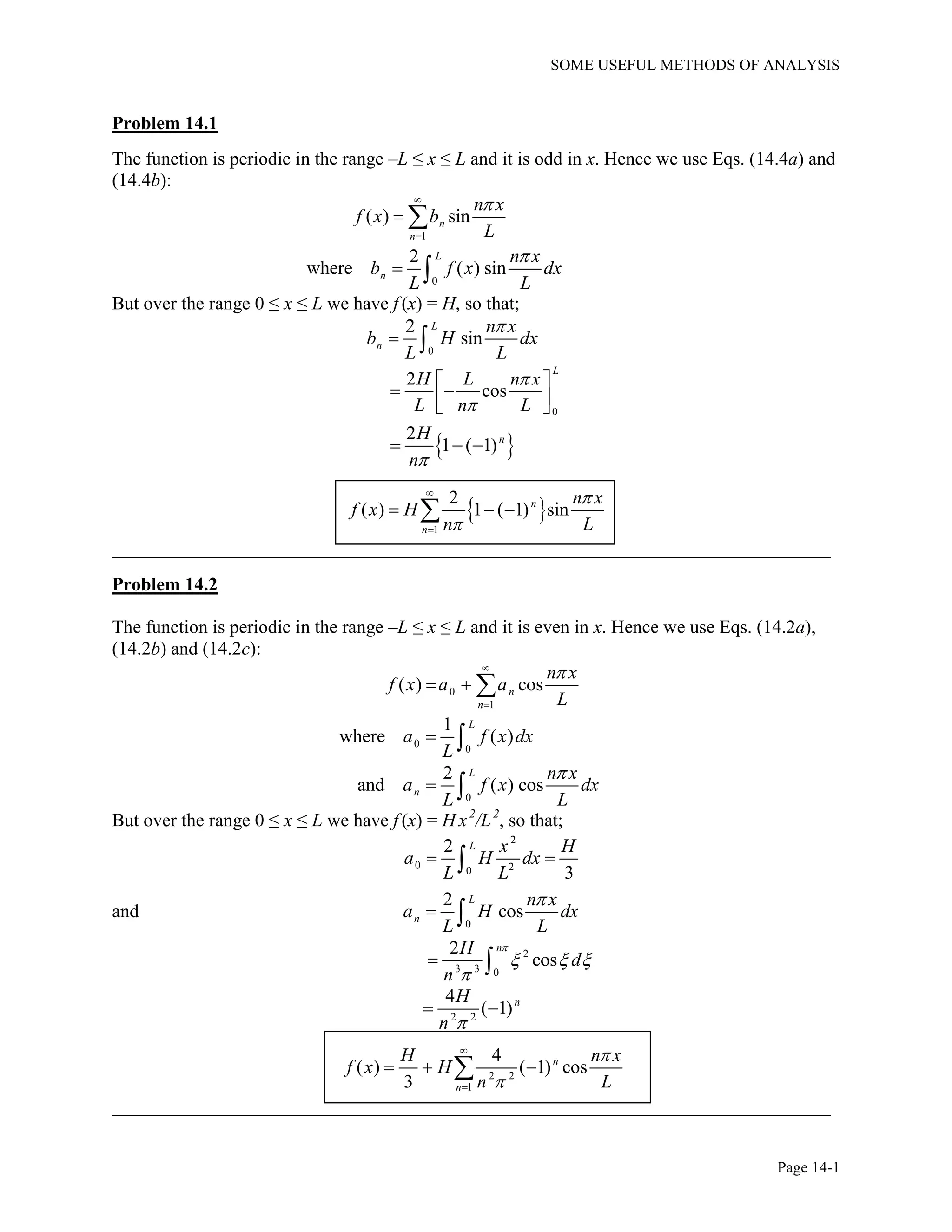
Problem 1.4
Using the given transformation equations gives:
2 2 2
2
2 2
and tan
2 2 2 cos cos
1 sin 1
and sec sin
cos
y
R x y
x
R R
R x R
x x
y
x x R x R
Using these results, the derivatives with respect to andx y transform as follows:
sin
cos
cos
sin
R
x x R x R R
R
y y R y R R
z z
Using these results and the relationships between the Cartesian and cylindrical vector
components, we get the following expressions for the Cartesian terms in the continuity equation:
sin
( ) cos [ ( cos sin )] [( ( cos sin )]R Ru u u u u
x R R
cos
( ) sin [ ( sin cos )] [( ( sin cos )]R Rv u u u u
y R R
Adding these two terms and simplifying produces the following equation:
1
( ) ( ) ( ) ( )
1 1
( ) ( )
R
R
R
u
u v u u
x y R R R
Ru u
R R R
Substituting this result into the full continuity equation yields the following result:
1 1
( ) ( ) ( ) 0R zRu u u
t R R R z
](https://image.slidesharecdn.com/solutionmanualforfundamentalmechanicsoffluidsbyi-180102082046-180117062948/75/fuandametals-of-fluid-mechanics-by-I-G-Currie-solution-manual-10-2048.jpg)

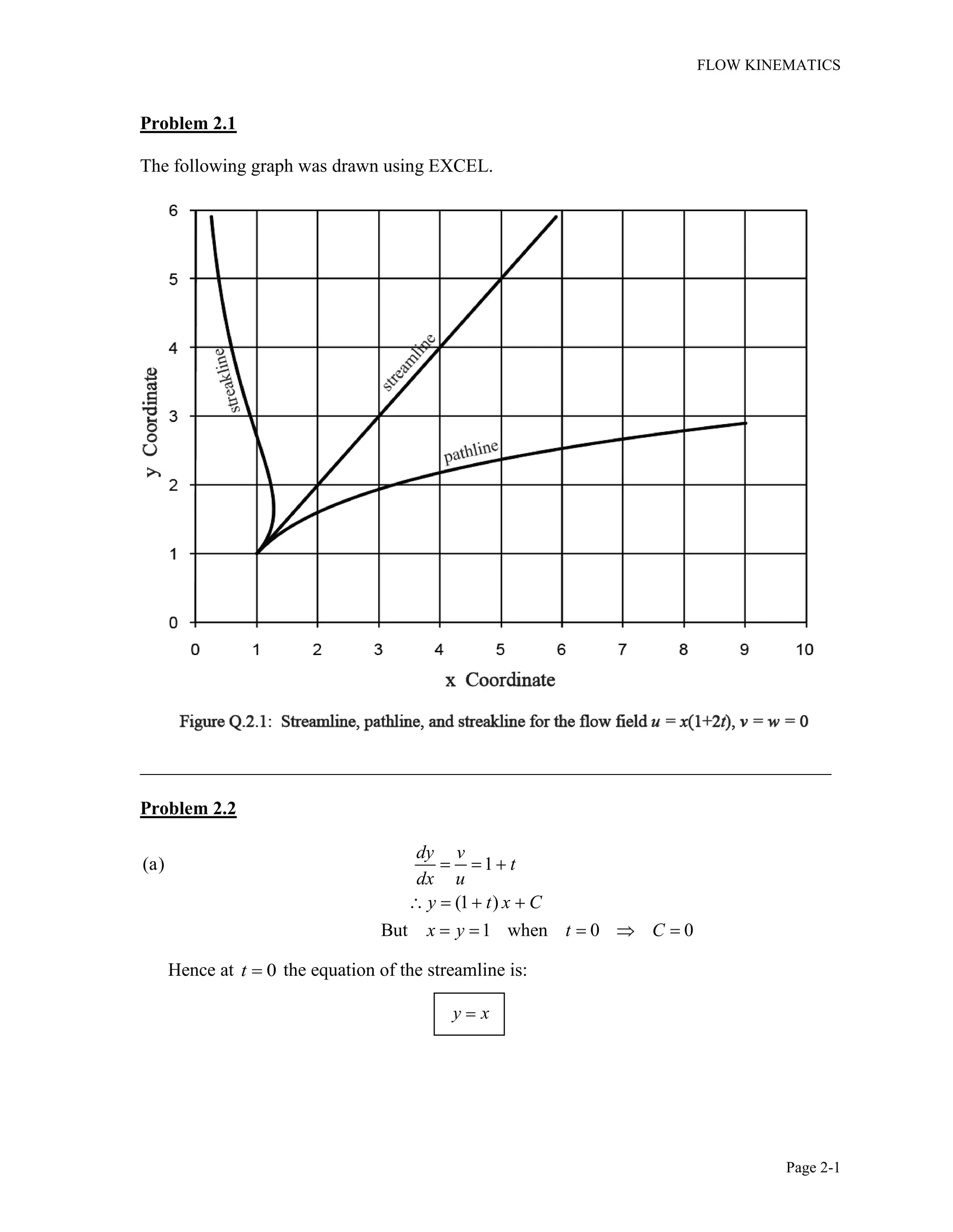
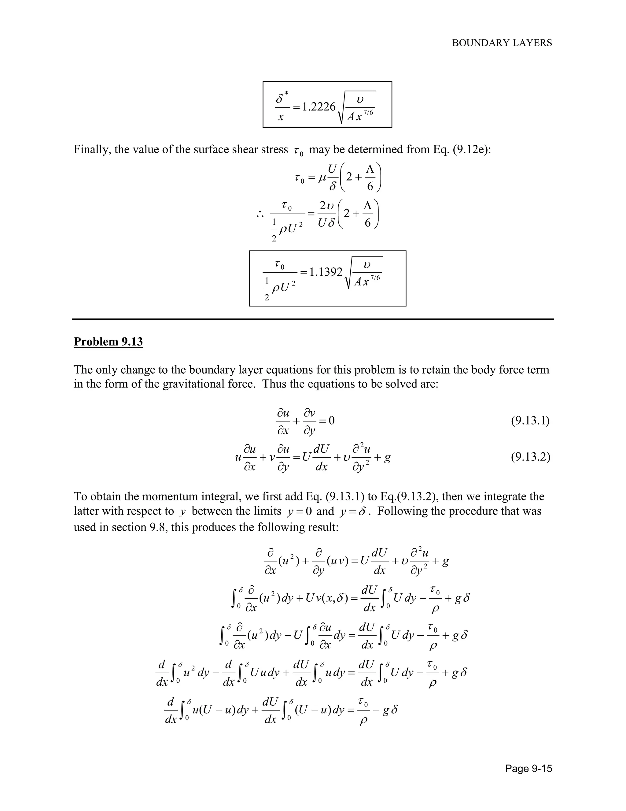
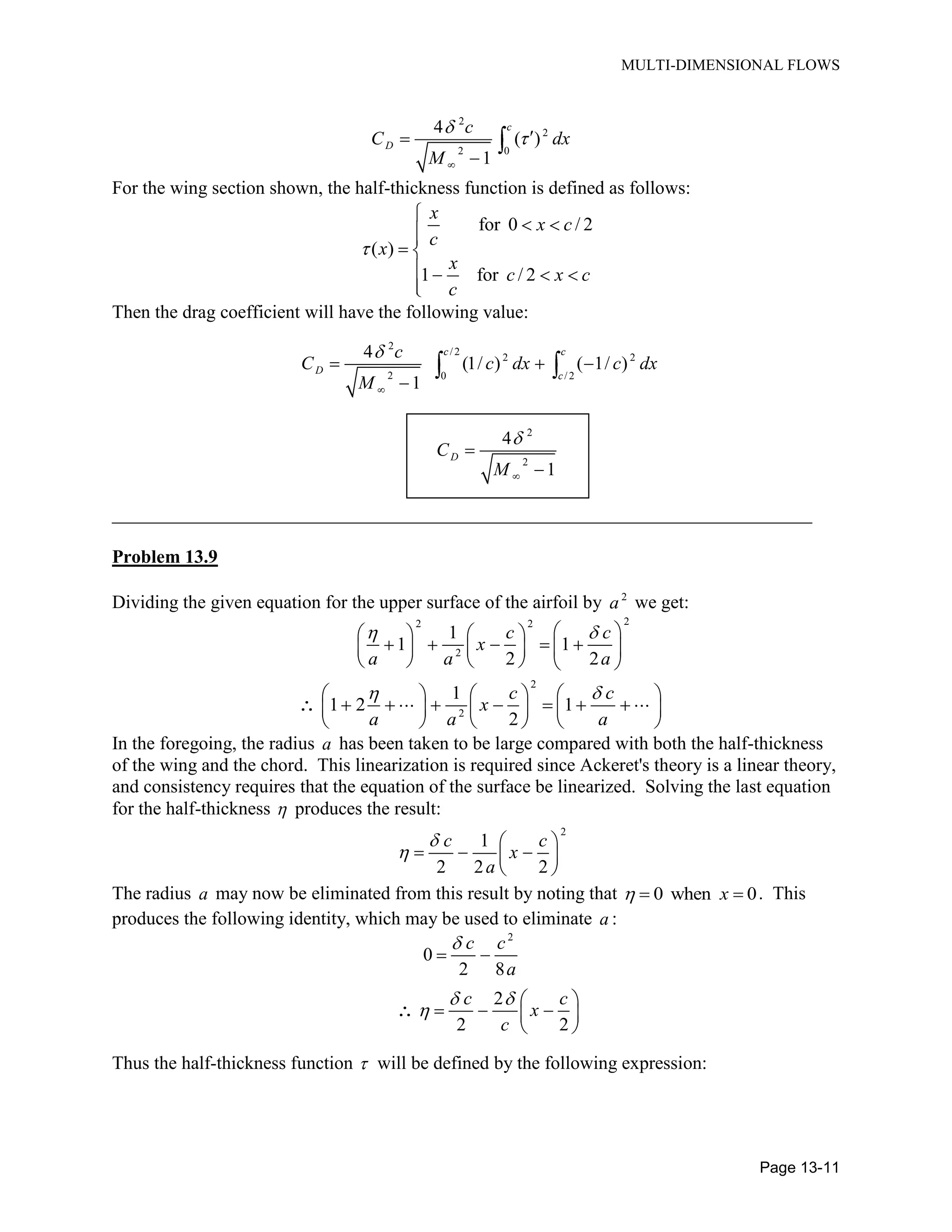
![FLOW KINEMATICS
Page 2-5
50
A
dAω n
This is the same result that was obtained in (a), so that Eq. (2.5) is verified for this flow.
Problem 2.6
2 2 2 2
and
x y
u v
x y x y
1 1 1 1
1 1 1 1
1 1 1 1
2 2 2 21 1 1 1
( , 1) ( 1, ) ( , 1) ( 1, )
1 1 1 1
u x dx v y dy u x dx v y dy
xdx y dy xdx y dy
x y x y
In the foregoing equation, we note that there are two pairs of offsetting integrals. Hence:
0
Problem 2.7
(a) 2 2
9 2 10 2u x y v x w yz
11 1
2 3
1 1 1
( , 1) (9 2) [3 2 ] 2u x dx x dx x x
11 1
1 1 1
( 1, ) 10 [10 ] 20v y dy dy y
11 1
2 3
1 1 1
( , 1) (9 2) [3 2 ] 10u x dx x dx x x
11 1
1 1 1
( 1, ) ( 10) [ 10 ] 20v y dy dy y
Hence: 2 20 10 20 32du l
(b) 2
2 8x y z x z
w v u w v u
z
y z z x x y
ω e e e e e
Hence 50 8x zω e e on the plane 5z](https://image.slidesharecdn.com/solutionmanualforfundamentalmechanicsoffluidsbyi-180102082046-180117062948/75/fuandametals-of-fluid-mechanics-by-I-G-Currie-solution-manual-23-2048.jpg)
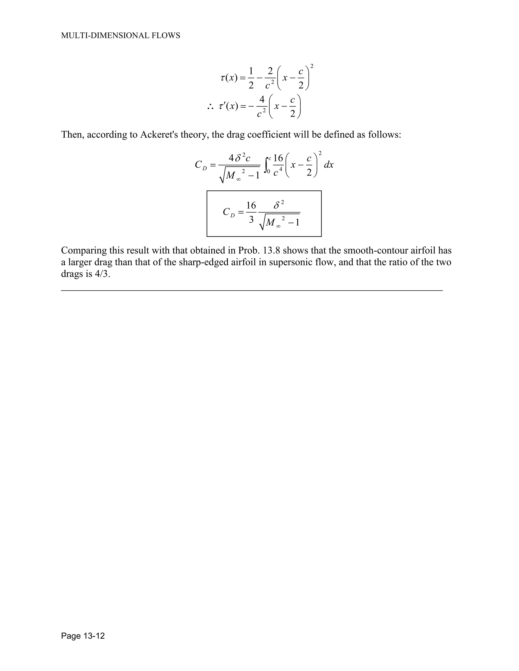
![FLOW KINEMATICS
Page 2-6
(c) For the plane 5z the unit normal is zn e . Hence:
1 1
1 1
8 32
A
dA dx dyω n
This agrees with the result obtained in (a) - as it should, since
A
d dAu l ω n
Problem 2.8
2 2 2 2
and
y x
u v
x y x y
1 1 1 1
1 1 1 1
1 1 1 1
2 2 2 21 1 1 1
1
1 1
121
(a) ( , 1) ( 1, ) ( , 1) ( 1, )
1 1 1 1
4 4[tan ]
1
u x dx v y dy u x dx v y dy
dx dy xdx dy
x y x y
d
2
2 2
2 2 2 2 2 2 2 2 2 2
(b)
1 2 1 2
( ) ( ) ( ) ( )
v u
x y
x y
x y x y x y x y
0 provided and 0x y
2 2 2 2 2 2
2 2
(c) and
( ) ( )
u x y v x y
x x y y x y
0 provided and 0x yu](https://image.slidesharecdn.com/solutionmanualforfundamentalmechanicsoffluidsbyi-180102082046-180117062948/75/fuandametals-of-fluid-mechanics-by-I-G-Currie-solution-manual-24-2048.jpg)
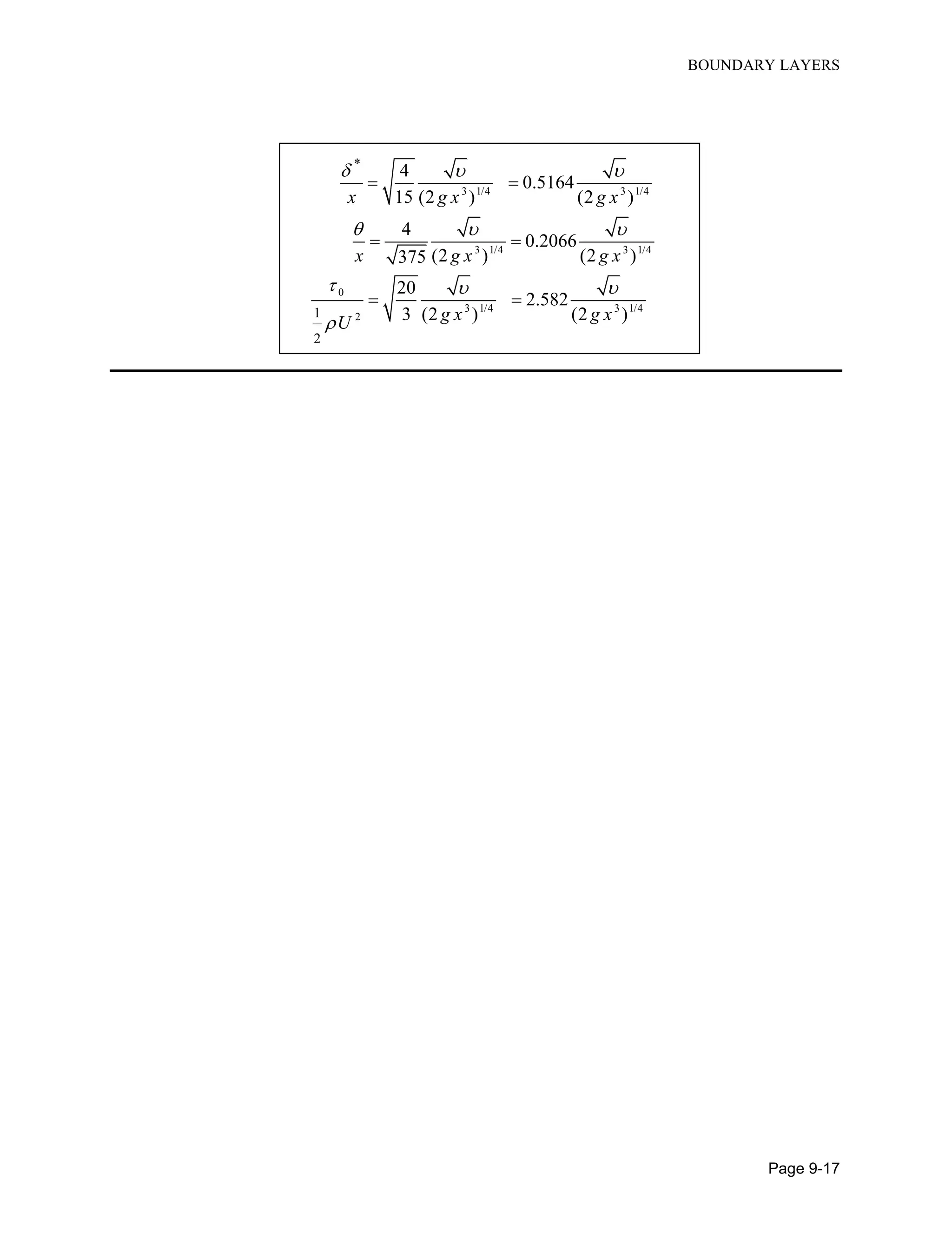
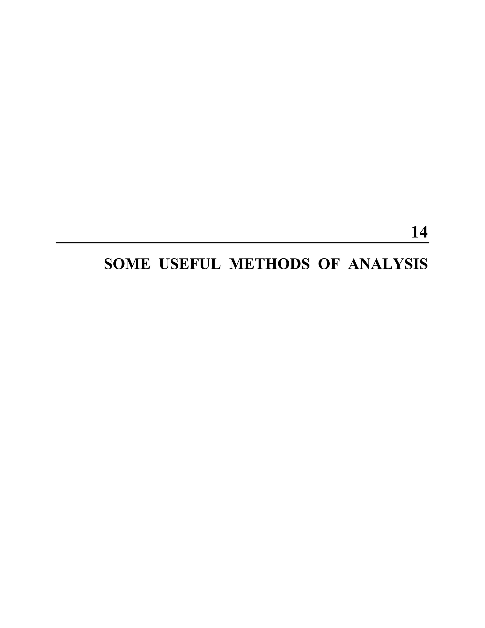
![FLOW KINEMATICS
Page 2-7
Problem 2.9
;u y v x
(a)
1 1 1 1
1 1 1 1
d ( ) ( )dx dy dx dyu
1 1 1 1
1 1 1 1
2 2 2 2
[ ] [ ] [ ] [ ]y yx x
4( )
(b) ( )
A
v u
ndA dxdy dxdy
x y
4( )
A
ndA
(c) and
dx dy
y x
ds ds
or
dy x
y dy xdx
dx y
2 2 2
2 2 2
y x c
2 2 2
x y c
(d) 2 2 2
1 and 1 x y c where andu y v x .
But x = 1 when y = 0 so that c 2
= 1. Therefore;
2 2
1x y
(e) 2 2 2
1 x y c where andu y v x .
But x = 0 when y = 0 so that c = 0. Therefore;
y x](https://image.slidesharecdn.com/solutionmanualforfundamentalmechanicsoffluidsbyi-180102082046-180117062948/75/fuandametals-of-fluid-mechanics-by-I-G-Currie-solution-manual-25-2048.jpg)


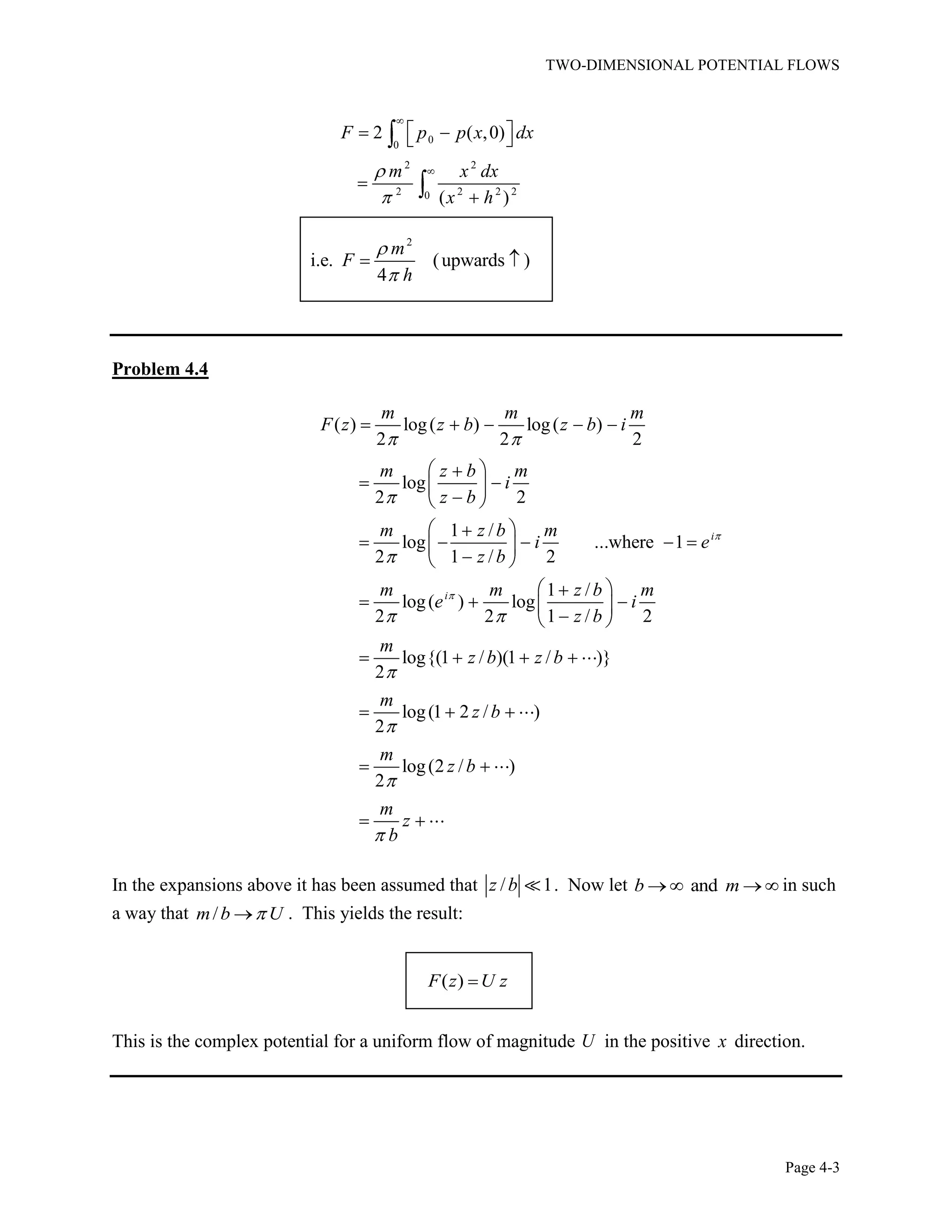
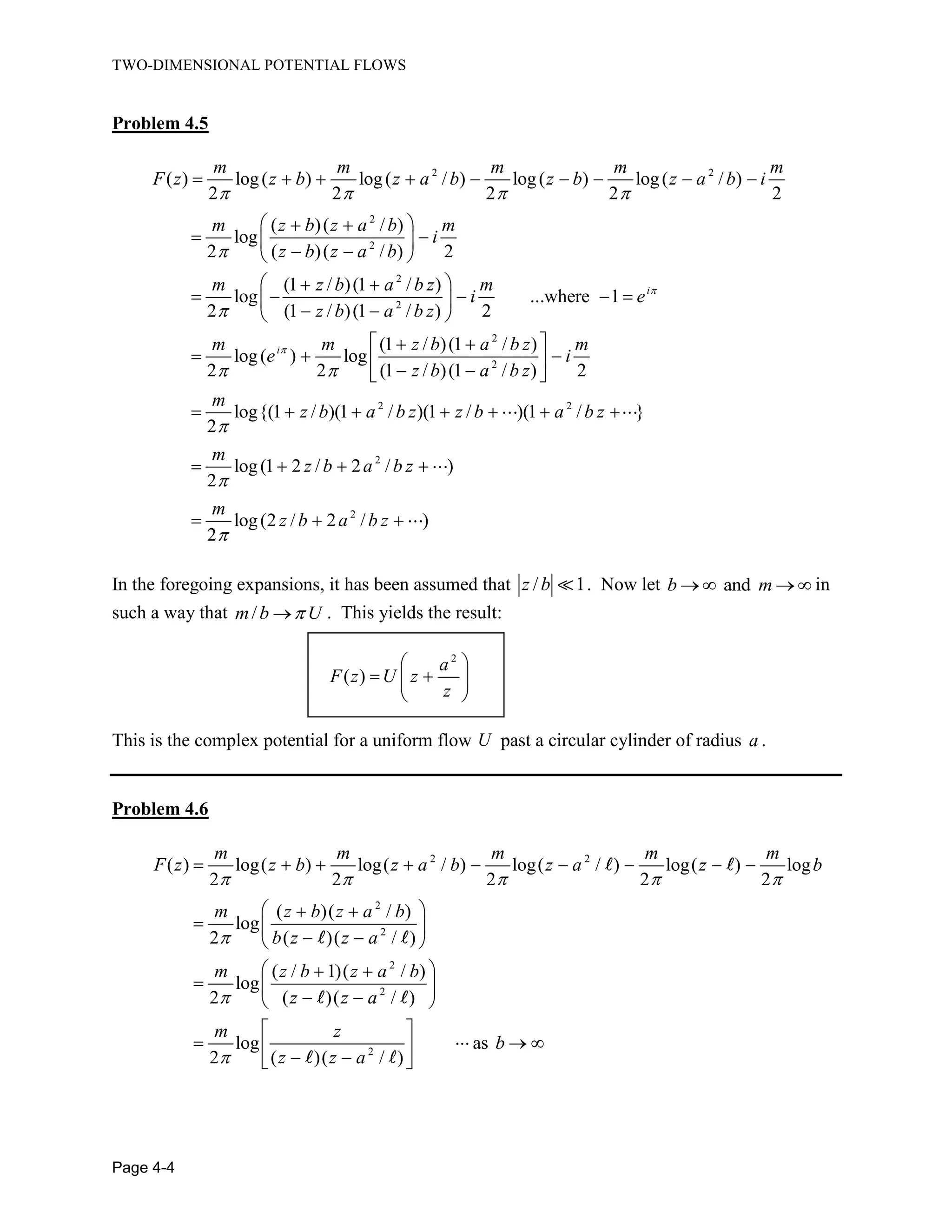
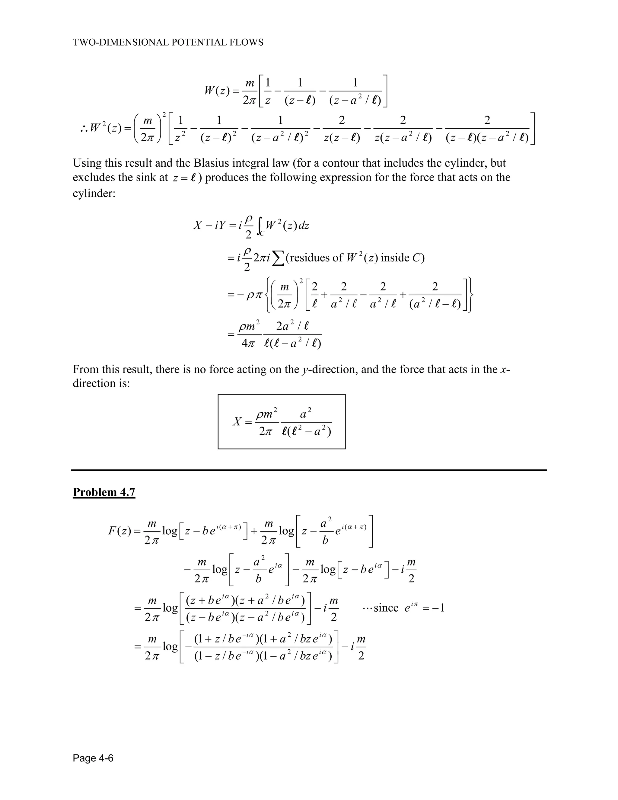
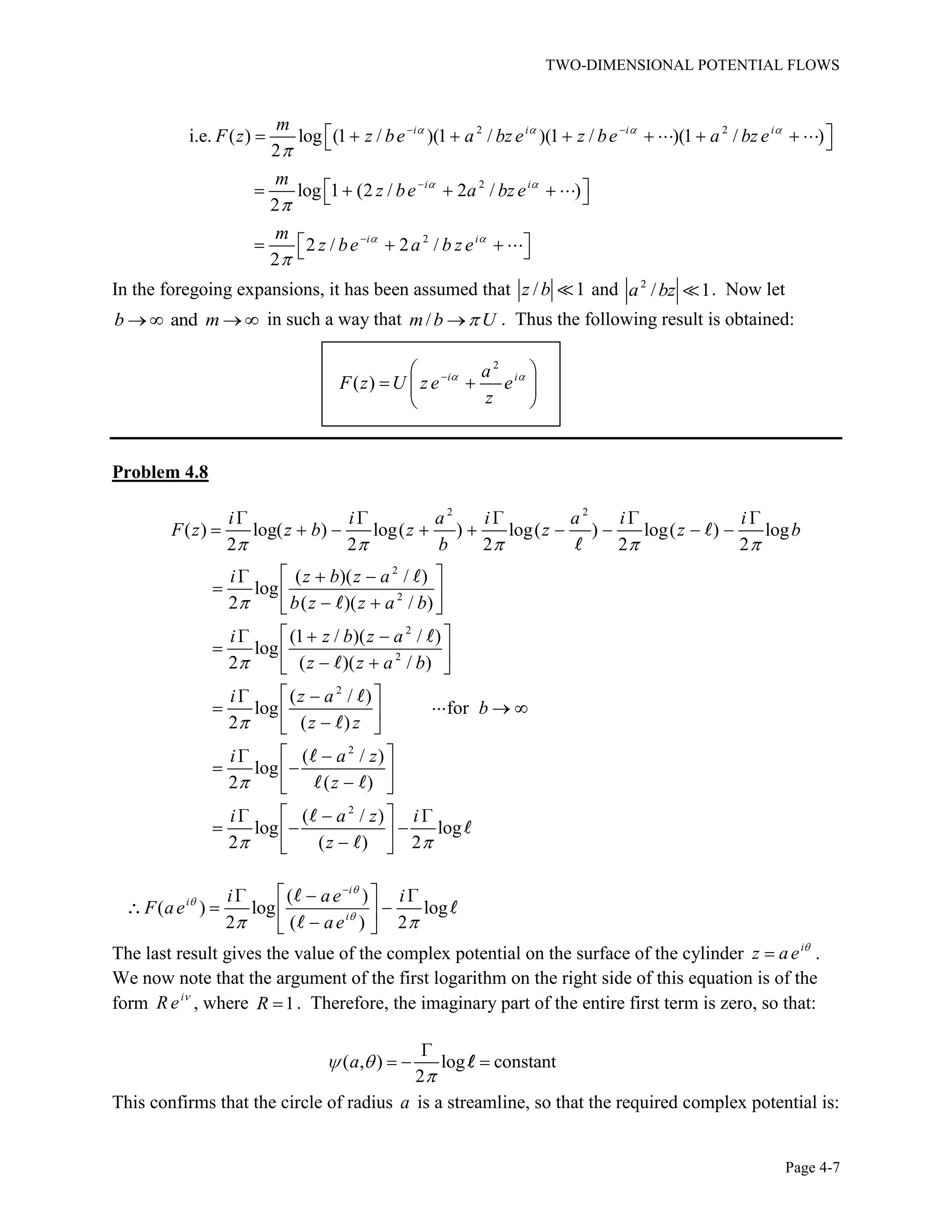
![TWO-DIMENSIONAL POTENTIAL FLOWS
Page 4-5
2 2
2 2
1
i.e. ( ) log
2 ( / ) / )
log[ ( / ) / )]
2
m
F z
z a a z
m
z a a z
On the surface of the circle of radius a this result becomes:
2
2 2
( ) log[ ( / ) )]
2
log[2 cos ( / )] log{ [( / ) 2 cos ]
2 2
i i i
i
m
F ae ae a ae
m m
a a e a a
2
log{( / ) 2 cos }
2 2
m m
a a i
For a , 2
( / ) 2a a so that 2
/ 2 cosa a and so / 2m . Therefore the
circle of radius a is a streamline. The required complex potential is given by:
2
( ) log
2 ( )( / )
m z
F z
z z a
The resulting flow field is illustrated below.
To determine the force acting on the cylinder, we calculate the complex velocity:](https://image.slidesharecdn.com/solutionmanualforfundamentalmechanicsoffluidsbyi-180102082046-180117062948/75/fuandametals-of-fluid-mechanics-by-I-G-Currie-solution-manual-37-2048.jpg)


![THREE-DIMENSIONAL POTENTIAL FLOWS
Page 5-8
At 0t the foregoing expression becomes:
2 3/2
1/2
3
2
1
0 ( )
d
RR R R R
R dt
Integrating this equation once with respect to r produces the following result:
3/2 3/2
0 0constantR R R R
3/2
0 0
3/2
3/2
3/2
0 0
hence
1
and
R RdR
dt R
dt R dR
R R
Evaluating the foregoing integrals between the limits of 0 and t for time, and 0 and 0R for the
radius R , we get the result:
0
0
2
5
R
t
R
Problem 5.8
Eq. (5.9b) defines the velocity potential for a uniform flow of magnitude U approaching a
sphere of radius a in the positive x -direction. If we replace U with U in this expression, we
will get the velocity approaching the sphere in the negative x -direction. Then, if we add a
uniform flow in the positive x -direction, the result will correspond to a sphere that is moving
with velocity U in an otherwise quiescent fluid. The resulting velocity potential is:
3
2
1
2
( , ) cos (5.8.1)
U a
r
r
In the foregoing equation, , andU r are all considered to be functions of time. In order to
switch to coordinates andx R, where both of these coordinates do not vary with time, we use
the relations:
2 2 1/2
0 0( ) cos and [ ( ) ]x x r r R x x
Substituting these expressions into Eq. (5.8.1) we get the following result:
03
2 2 3/2
0
1
2
( )
( , ) (5.8.2)
[ ( ) ]
x x
x R U a
R x x
In the foregoing, 0andU x are both considered to be functions of time, but all of the other
quantities are time-independent. To obtain an expression for the pressure, we employ
Bernoulli’s equation in the form defined by Eq. (3.2c) in which the quantity ( )F t is evaluated](https://image.slidesharecdn.com/solutionmanualforfundamentalmechanicsoffluidsbyi-180102082046-180117062948/75/fuandametals-of-fluid-mechanics-by-I-G-Currie-solution-manual-64-2048.jpg)

![SURFACE WAVES
Page 6-4
2
( ) cos ( )
sinh (2 / )
c
F z z ct i h
h
We change the speed from c to U , and the liquid depth from h to H . At the same time, we
superimpose a uniform flow of magnitude U in the negative x -direction to account for the fact
that we are observing the flow from a frame of reference that is moving with the wave; that is,
with velocity U in the positive x -direction. Then the wave will appear to be stationary, and the
originally-quiescent liquid will appear to be approaching us in the negative x -direction. Also,
the distance z from the fixed origin will change such that z ct z . The resulting complex
potential is:
2
( ) cos ( )
sinh (2 / )
2
( ) cos [ ( )]
sinh (2 / )
2 2 2 2
( ) cos cosh ( ) sin sinh ( )
sinh (2 / )
U
F z U z z i H
H
U
U x i y x i y H
H
U x x
U x i y y H i y H
H
Hence the stream function for the flow will be:
2 2
( , ) sin sinh ( )
sinh(2 / )
U x
x y U y y H
H
The relationship connecting the mean liquid speed, the liquid depth, and the wavelength of the
surface wave is given by Eq. (6.3a) in which c is replaced by U and the depth h is replaced by
H . This gives:
2
2
tanh
2
U H
g H H
Problem 6.5
Put U h when 0 sin(2 / )y h x in the expression obtained in Prob. 6.4 for the
stream function. This produces the following equation:
0 0
2
0 sinh [( ) sin 2 / ]
sinh(2 / )
U
U H h x
H
Consider 0 ( )H h and solve this equation for the amplitude ratio, to get:
0
sinh (2 / )
sinh 2 ( )/
1
cosh (2 / ) coth (2 / ) sinh (2 / )
H
H h
h H h
](https://image.slidesharecdn.com/solutionmanualforfundamentalmechanicsoffluidsbyi-180102082046-180117062948/75/fuandametals-of-fluid-mechanics-by-I-G-Currie-solution-manual-72-2048.jpg)

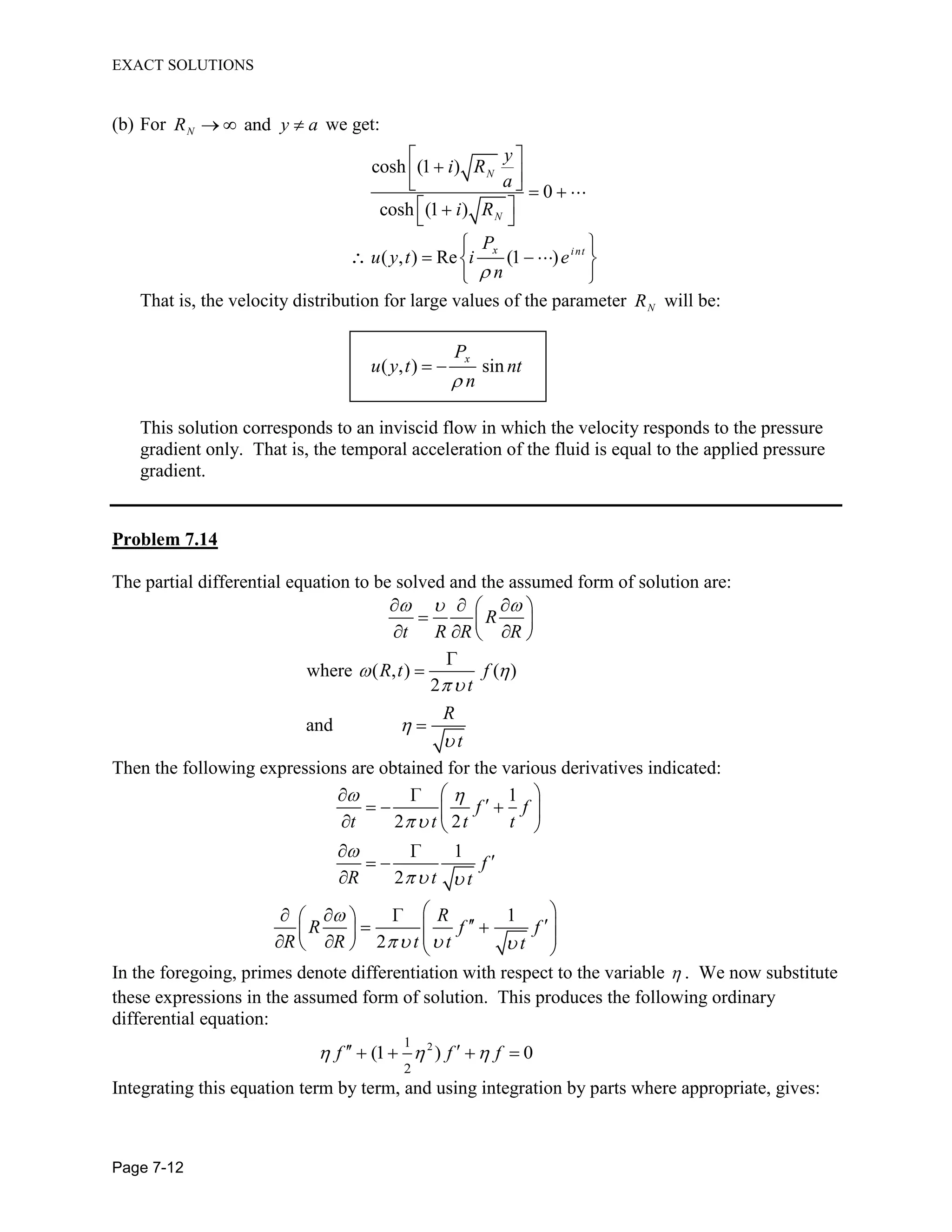
![EXACT SOLUTIONS
Page 7-7
Problem 7.8
The only non-zero component of velocity in this case will be ( , )u y z and this velocity
component will be the solution to the following reduced form of the Navier-Stokes equations:
2 2
2 2
0
u u
y z
with ( , ) 0u y
and
1
2
( ,0) [1 ( 1) ]sinn
n
n y
u y U U
n b
In the foregoing, the boundary condition on 0z has be written in terms of the Fourier series
for a square wave of height U . The solution to this problem may be obtained by separation of
variables. In this solution, the y -dependence will be trigonometric and the z -dependence will
be exponential. Hence, the solution will be:
1
2
( , ) [1 ( 1) ] sin
n z
n b
n
n y
u y t U e
n b
The volumetric flow rate Q may be evaluated by integrating the velocity to give:
0 0
1
2
2 20
1
2
1 ( 1) sin
2
1 ( 1)
n z
b
n b
n
n z
n b
n
n y
Q dz U e dy
n b
b
U e dz
n
Thus the volumetric flow rate past any vertical plane across the flow will be:
22
3 3
1
2
1 ( 1)n
n
Q U b
n
Problem 7.9
(a)
1 1d dw dp
R
R dR dR dz
Fluid #1:
2
1 1 1
1
1
( ) log
4
dp R
w R A R B
dz
Fluid #2:
2
2 2 2
2
1
( ) log
4
dp R
w R A R B
dz
The fact that 1( )w R should be finite when 0R requires that the constant 1 0A . Also,
matching the shear stresses at 1R R produces the following result:](https://image.slidesharecdn.com/solutionmanualforfundamentalmechanicsoffluidsbyi-180102082046-180117062948/75/fuandametals-of-fluid-mechanics-by-I-G-Currie-solution-manual-87-2048.jpg)

![LOW-REYNOLDS-NUMBER SOLUTIONS
Page 8-7
2 1
0
t
The boundary conditions to be satisfied by the velocity on the surface of an oscillating sphere of
radius a , and also far from the sphere, are as follows:
( , ) cos ( ) (8.4.1 )
( , ) finite as (8.4.1 )
ra t a t a
r t r b
u e
u
In consideration of Eq. (8.4.1a) it is clear that the velocity, and the function , will both be
functions of andr t only. Furthermore, the time dependence will be defined by the time
dependence of the sphere’s motion. However, the possibility of a phase lag exists in the r -
dependence. Then the partial differential equation to be solved for the function will be:
2
2
1 1
0
where ( , ) Re{ ( ) }i t
r
r r r t
r t R r e
Substituting the assumed form of solution into the partial differential equation gives:
2
2
1
0
d dR
r i R
r dr dr
This differential equation may be simplified by introducing a new dependent variable r R .
Then the differential equation becomes:
2
2
0
d
i
dr
Thus the solution to the original differential equation is seen to be:
/ ( ) / ( )1
( ) i r a i r a
R r Ae Be
r
In order to satisfy the boundary condition (8.4.1b) we must choose 0B . Hence the solution
for the function ( , )r t becomes:
/ ( )
/2 ( ) [ /2 ( )]
( , ) Re
Re
i r a i t
r a i r a
A
r t e e
r
A
e e
r
In the foregoing, we have used the fact that (1 )/ 2i i . In terms of the function ( , )r t ,
the boundary condition (8.4.1a) is:
( , ) Re{ }i t
a t ae
Imposing this boundary condition on the solution establishes the value for the constant A to be
2
A a . Then:
2
[ /2 ( )]/ ( )
( , ) Re i t r ar aa
r t e e
r
Then the velocity distribution in the fluid will be defined by the following expressions:](https://image.slidesharecdn.com/solutionmanualforfundamentalmechanicsoffluidsbyi-180102082046-180117062948/75/fuandametals-of-fluid-mechanics-by-I-G-Currie-solution-manual-105-2048.jpg)
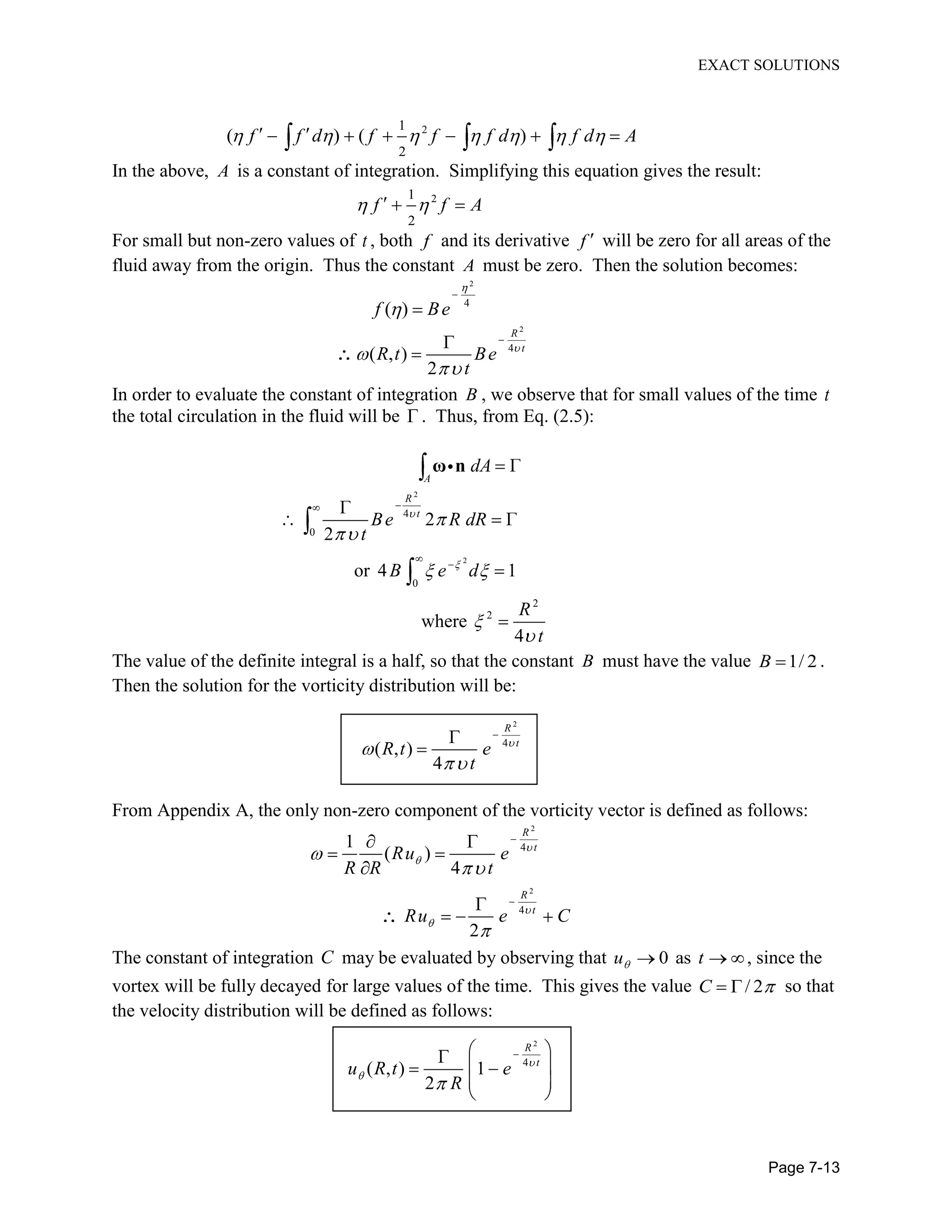
![LOW-REYNOLDS-NUMBER SOLUTIONS
Page 8-8
2
/ ( )
where ( , ) cos[ / 2 ( )]r aa
r t e t r a
r
u
Problem 8.5
In spherical coordinates, the vorticity vector and the Stokes stream function for any
axisymmetric flow are defined as follows:
2
1 1
( )
1
sin
1
sin
r
r
u
r u
r r r
u
r
u
r r
e
Substitution of the last two expressions into the first gives:
2
2 2
2
2
2
2 2
1 sin 1
sin sin
1
i.e.
sin
sin 1
where
sin
r r r
L
r
L
r r
e
e
The quantity 2
L in the foregoing is a linear, second-order differential operator that is similar to,
but not equal to, the Laplacian operator. We next take the curl of twice and invoke standard
vector identities as follows:
2 2
2
2
2 2
2 2
2 2
1 1
( ) ( )
sin sin
1 sin 1
( ) ( )
sin sin
1
( )
sin
rL L
r r r
L L
r r r
L L
r
e e
e
e
The following vector identities, and the Stokes equations, are now used to show that the left side
of the last equation is zero:](https://image.slidesharecdn.com/solutionmanualforfundamentalmechanicsoffluidsbyi-180102082046-180117062948/75/fuandametals-of-fluid-mechanics-by-I-G-Currie-solution-manual-106-2048.jpg)
![LOW-REYNOLDS-NUMBER SOLUTIONS
Page 8-9
2
[ ( ) ]
)
0
p
u u
= (
That is, the partial differential equation that is to be satisfied by the Stokes stream function, for
any pressure distribution, is:
2 2
( ) 0L L
2
2
2 2
sin 1
where
sin
L
r r
_____________________________________________________________________________
Problem 8.6
A solution to the partial differential equation obtained in Prob. 8.5 above is now sought in the
following form:
( , ) ( )r r f
Substituting this assumed form of solution into the partial differential equation shows that:
4 2
3 4 2
1
2 0
d f d f
f
r dr dr
The general form of the solution to this equation is:
( ) sin cos sin cosf A B C D
The boundary conditions that must be satisfied by this solution are the following:
( ,0) 0 (0) 0
1
( ,0) (0)
( , / 2) 0 ( / 2) 0
1
( , / 2) 0 ( / 2) 0
r f
r
r U f U
r
r f
r
r f
r
Imposing these boundary conditions leads to the following four algebraic equations that are to be
satisfied:](https://image.slidesharecdn.com/solutionmanualforfundamentalmechanicsoffluidsbyi-180102082046-180117062948/75/fuandametals-of-fluid-mechanics-by-I-G-Currie-solution-manual-107-2048.jpg)


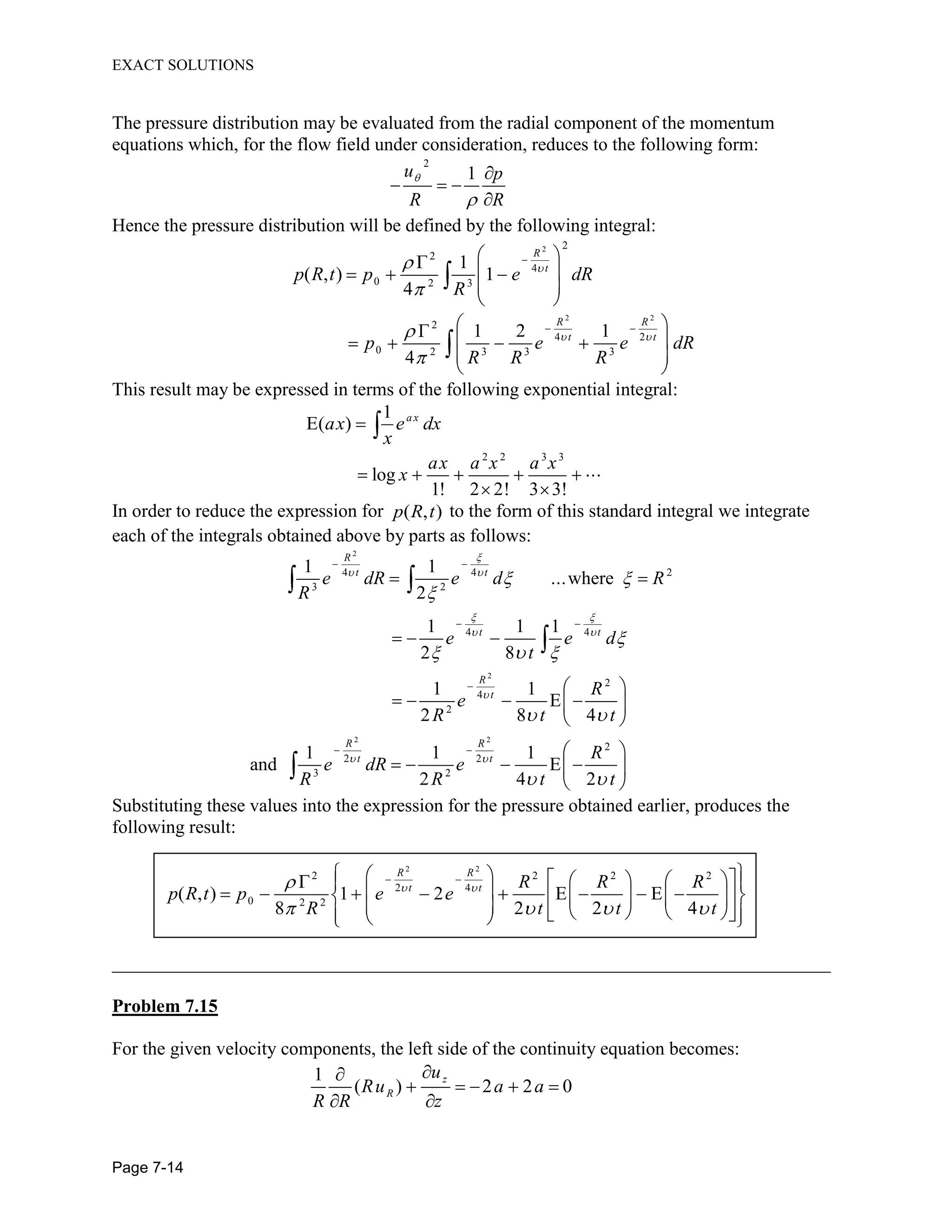
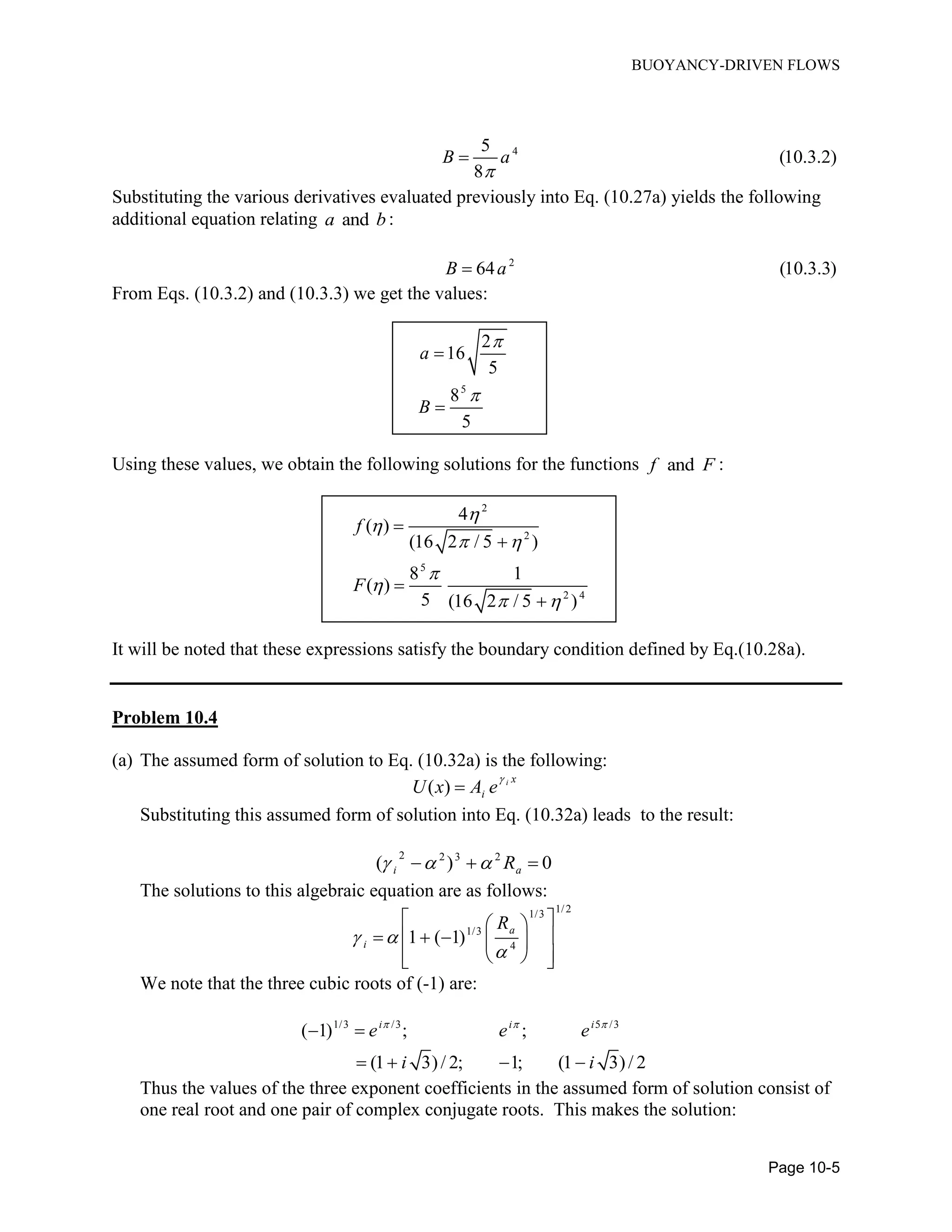
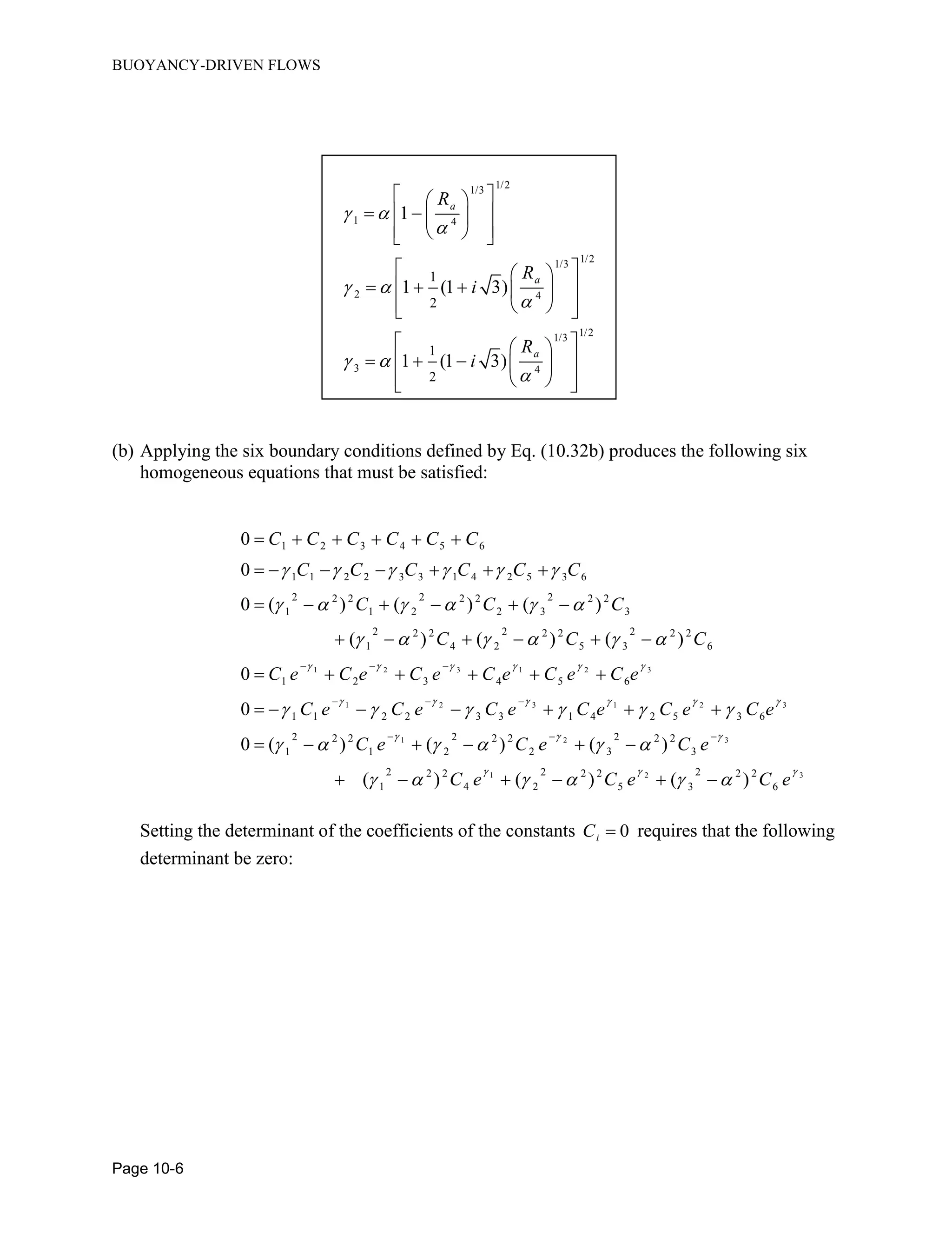
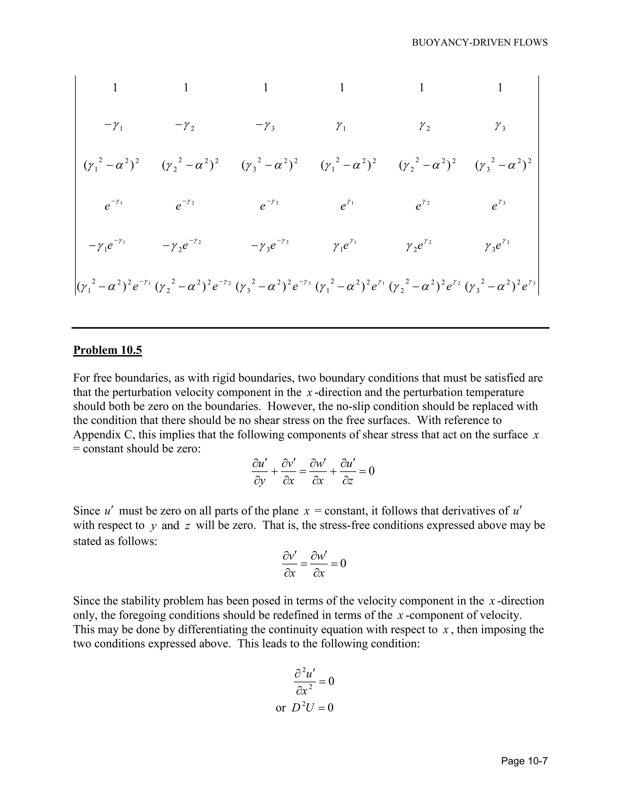
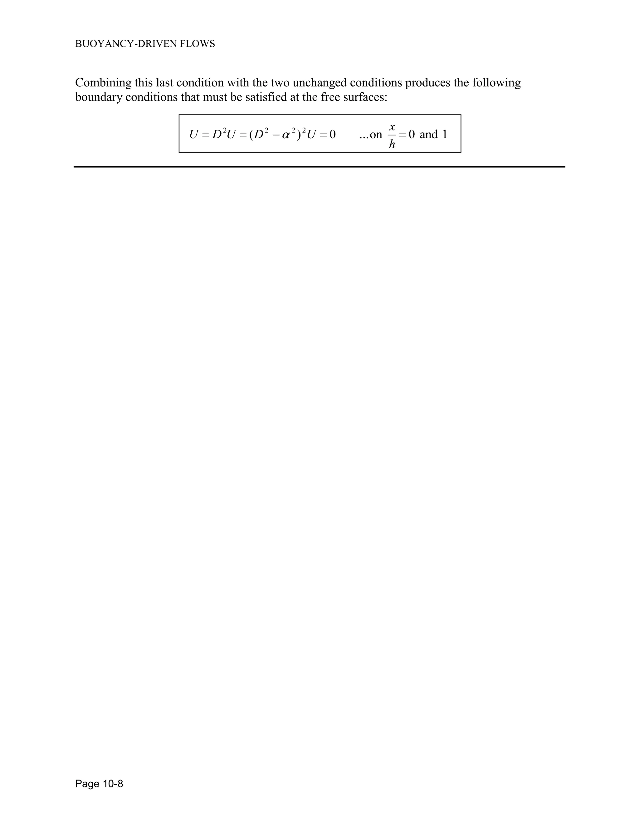
![BUOYANCY-DRIVEN FLOWS
Page 10-1
Problem 10.1
From section 10.6 of the text, the partial differential equations to be satisfied are as follows:
1 1 1 1 1
(10.1.1)
(10.1.2)
R g
R R x R R R x R R R R R R R R
R
R x x R R R
Using the given expressions, the following derivatives are obtained:
1
1
1 2
2
1
1 2
2
2 2
1 22
3
3 3
1 23
1
3
2 3
2
2 2
2 32
( )
[ ( ) ]
( )
m
m n
m n
m n
m n
r
r n
m n
C x n f m f
x
C C x f
y
C C x n f m n f
x y
C C x f
y
C C x f
y
C x n F r F
x
C C x F
y
C C x F
y
Substituting these expressions into Eqs. (10.1.1) and (10.1.2) and simplifying yields:
2 2 1 2 2 2 1
1 2 1 2
32 3 3
1 2 3
2
( 2 ) ( ) ( )
( ) (10.1.3)
m n m n
m n r n
m n C C x f mC C x f f f f
C
C C x f f f g x F
C
1 1
1 2 3 1 2 3 2 3 ( ) (10.1.4)m n r m n r r n
C C C x r f F mC C C x f F C C x F F
If a similarity solution exists, all of the powers of x in Eq. (10.1.3) must be the same so that x
cancels out of the equation. This leads to the equations:
1 and 4 1m n r ](https://image.slidesharecdn.com/solutionmanualforfundamentalmechanicsoffluidsbyi-180102082046-180117062948/75/fuandametals-of-fluid-mechanics-by-I-G-Currie-solution-manual-131-2048.jpg)

![SHOCK WAVES
Page 11-3
0
0 0
de p
s s dv
T T
0
0 0
i.e. v
dT
s s C Rvdv
T
Integrating this equation and using the fact that 1/ v yields the result:
0
0
0
log logv
T
s s C R
T
Using the relation p vC C R in the foregoing result produces the equation:
0
0
0
0 0 0
( )log log
log log
p
p
T
s s C R R
T
T T
C R
T T
Hence, using the ideal gas law, the last equation becomes:
0
0 0
log logp
T p
s s C R
T p
Problem 11.4
[ ( ) ]
where ( , ) and ( , )
u f x u a t
u u x t a a x t
( )
and 1
u u a
f u a t
t t t
u u a
f t
x x x
hence ( ) ( ) ( )
u u u u a a
u a u a u a t f
t x t x t x
But we know that u is a function of and that a is also a function of , so that we may
consider a to be a function of u only. Hence:
a da u
t du t
a da u
x du x
Substituting these results into the differential expression above gives:](https://image.slidesharecdn.com/solutionmanualforfundamentalmechanicsoffluidsbyi-180102082046-180117062948/75/fuandametals-of-fluid-mechanics-by-I-G-Currie-solution-manual-143-2048.jpg)
![SHOCK WAVES
Page 11-4
( ) ( ) 1
u u u u da
u a u a t f
t x t x du
( ) 1 1 0
u u da
u a t f
t x du
Either the first curly bracket is zero or the second curly bracket is zero. In general, the latter
cannot be true since the equation is valid for all values of the time t, so that the first curly bracket
must be zero. That is, the following is the solution to the wave equation:
( , ) [ ( ) ]u x t f x u a t
Problem 11.5
( ) 0
u u
u a
t x
( ) 0
u u u a u
u a
t x x x x x x
or
D u u a u
Dt x x x x
The partial derivative of a with respect to x may be shown to be proportional to the partial
derivative of u with respect to x as follows. In section 11.2, the following relationships were
established:
1
2
0
0
3 3
2 2
0 0 0
0 0 0
hence
1
2
1
2
a a
d
du a
a da d u
x d du x
a u
a x
u
x
Substituting this expression into the equation for the steepness of the wave front gives:
2
1
2
D u u
Dt x x](https://image.slidesharecdn.com/solutionmanualforfundamentalmechanicsoffluidsbyi-180102082046-180117062948/75/fuandametals-of-fluid-mechanics-by-I-G-Currie-solution-manual-144-2048.jpg)


![ONE-DIMENSIONAL FLOWS
Page 12-6
Using the result of Prob. 12.4, and the result obtained above, yields the following expression:
32 2
2 1 1
2
1 2 2
1
1
M M
M M
Problem 12.6
Starting with the ideal gas law and employing the given expression for h , we get:
p
R
p RT h
C
Substituting this result into the given expression for the entropy rise produces the result:
1 1 1
1
1 1
log log
v p
s s p R h
C p p C
In order to eliminate , we use the energy equation and the continuity equation as follows:
2
0
2
0
1/2
0
2
1
2
1
[2( )]
u
h h
m
h h
A
A
h h
m
Substituting this result into our expression for the entropy change yields the result:
1
2 2
1 1
02
1
2
log ( )
v p
s s R A
h h h
C p C m
Separating the variable and the constant components of the last equation gives the result:
1
1 2 2
1 12
0 2
1
2
log ( ) log
v p
s s R A
h h h
C p C m
The maximum value of the entropy s will occur when the derivative of the right side of the last
equation, with respect to h , is zero. This requires the following:
1 3
2 2
0 01
2
0
1 1
( ) ( ) 0
2
( )
h h h h h
h h h
Simplifying this expression shows that it follows that:](https://image.slidesharecdn.com/solutionmanualforfundamentalmechanicsoffluidsbyi-180102082046-180117062948/75/fuandametals-of-fluid-mechanics-by-I-G-Currie-solution-manual-158-2048.jpg)


![MULTI-DIMENSIONAL FLOWS
Page 13-8
2 2 2 2 2
2 2 2
2
(2 ( ) ( ) ( ) [4 ( ) ]
2 8
pC U u u v w U u
M a a
Simplifying this expression yields the following equation which is valid to the second order in
the primed (i.e. small) quantities:
2 2
2
( ) ( )
2p
u u v
C
U U
Problem 13.6
The drag force that acts on one wave-length of wall is defined by the following integral:
0
0
( ,0)
2 2
( ,0)cos
D
dy
F p x dx
dx
x
p x dx
In the foregoing equation, ( ,0)p x is the pressure difference across the wavy wall, and the
sinusoidal variation of the wall height has been employed. It will be assumed that the pressure
below the wall surface is the same as the reference pressure far from the wall. For subsonic flow
the pressure coefficient is given by Eq. (13.6b). Hence the required pressure distribution will be
defined as follows:
22
1
2
4 / 2
( , ) sin
1
M y
p
x
C x y e
M
2
2
2 / 2
( ,0) sin
1
U x
p x
M
Thus for subsonic flow the drag force per unit wavelength of wall will be:
2 2
2 0
2 2 2
sin cos
1
D
U x x
F dx
M
i.e. 0 for 1DF M
For supersonic flow the pressure coefficient is defined by Eq. (13.7b). Hence the required
pressure distribution will be defined as follows:
2
2
4 / 2
( , ) cos 1
1
p
x
C x y x M y
M
2
2
2 / 2
( ,0) cos
1
U x
p x
M
Thus for supersonic flow the drag force per unit wavelength of wall will be:](https://image.slidesharecdn.com/solutionmanualforfundamentalmechanicsoffluidsbyi-180102082046-180117062948/75/fuandametals-of-fluid-mechanics-by-I-G-Currie-solution-manual-170-2048.jpg)


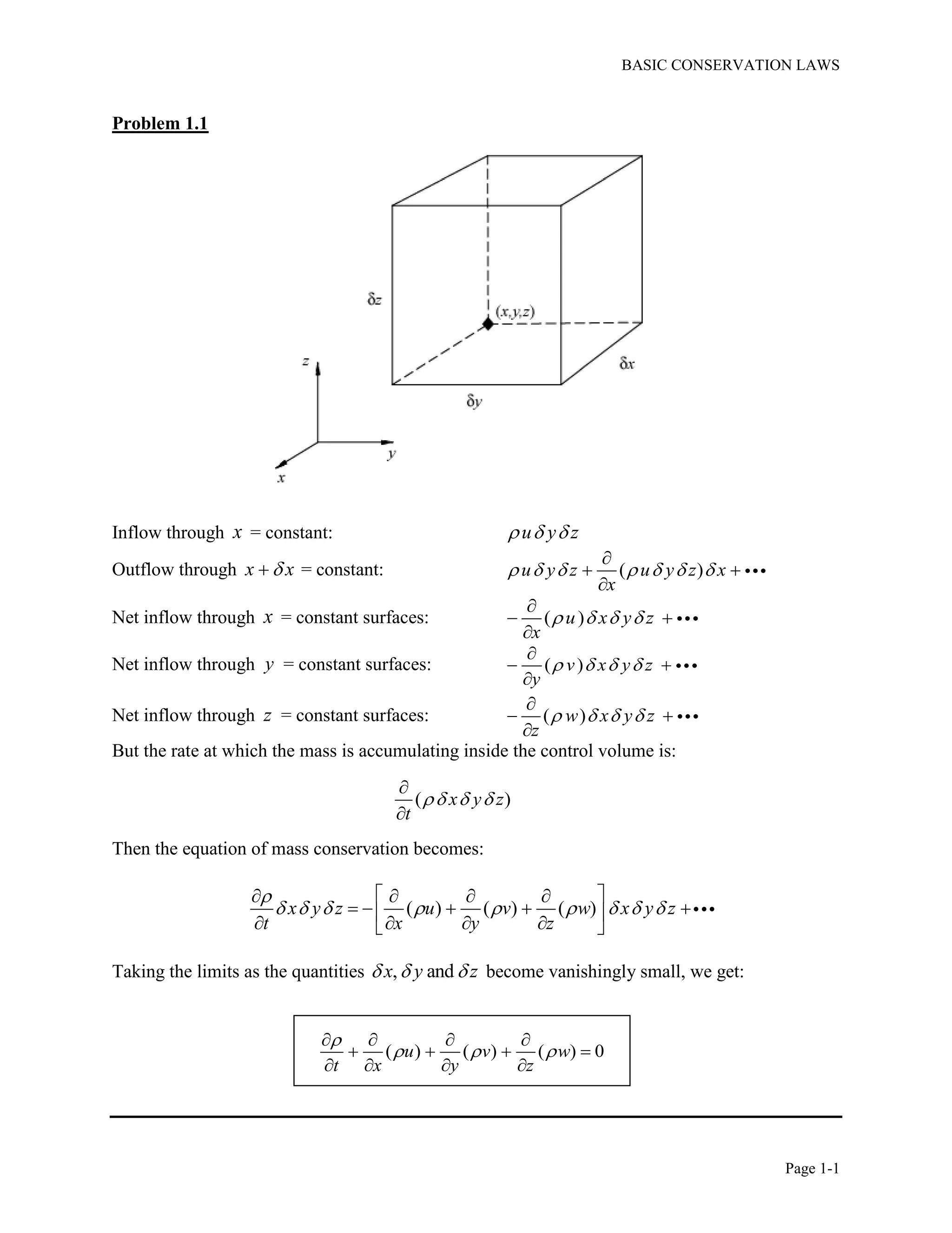
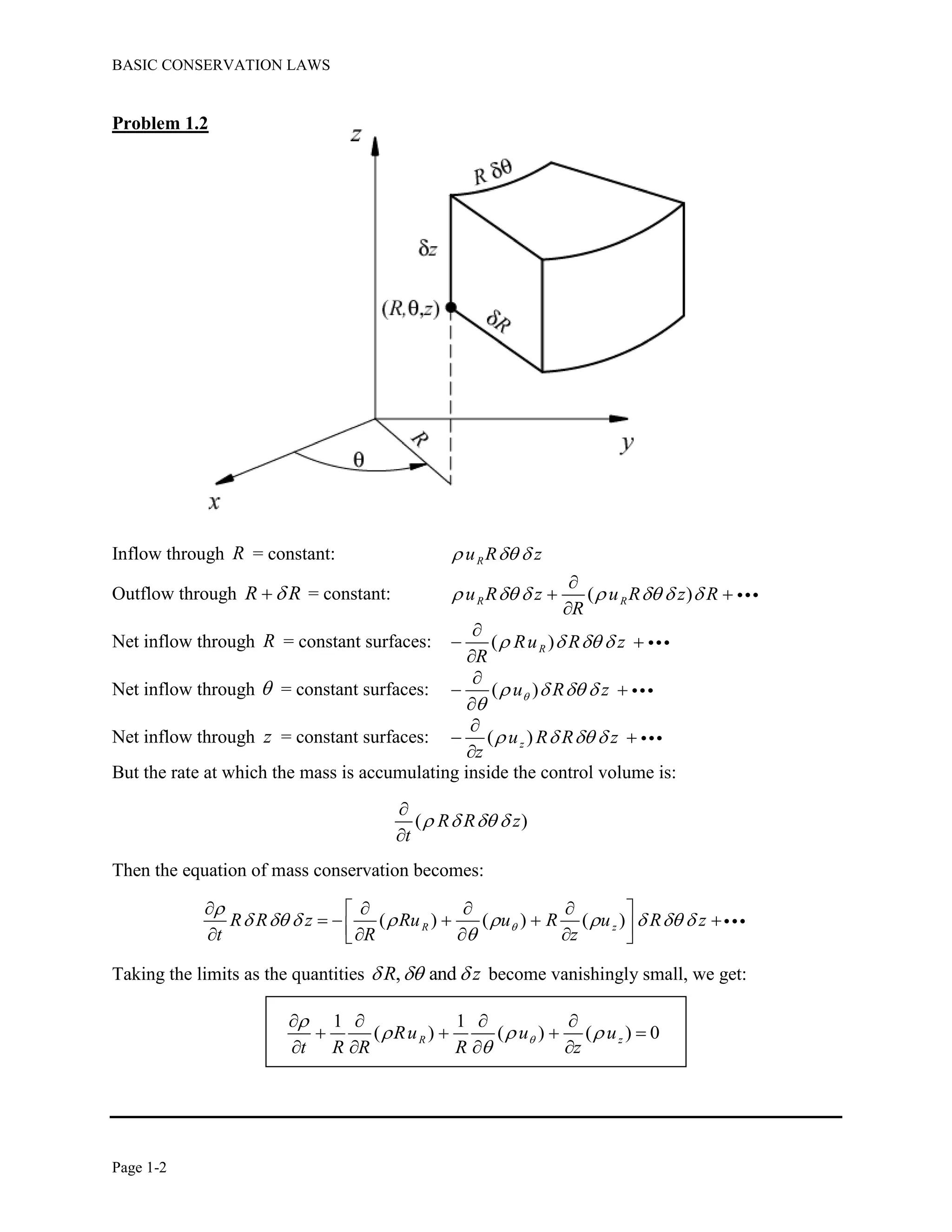
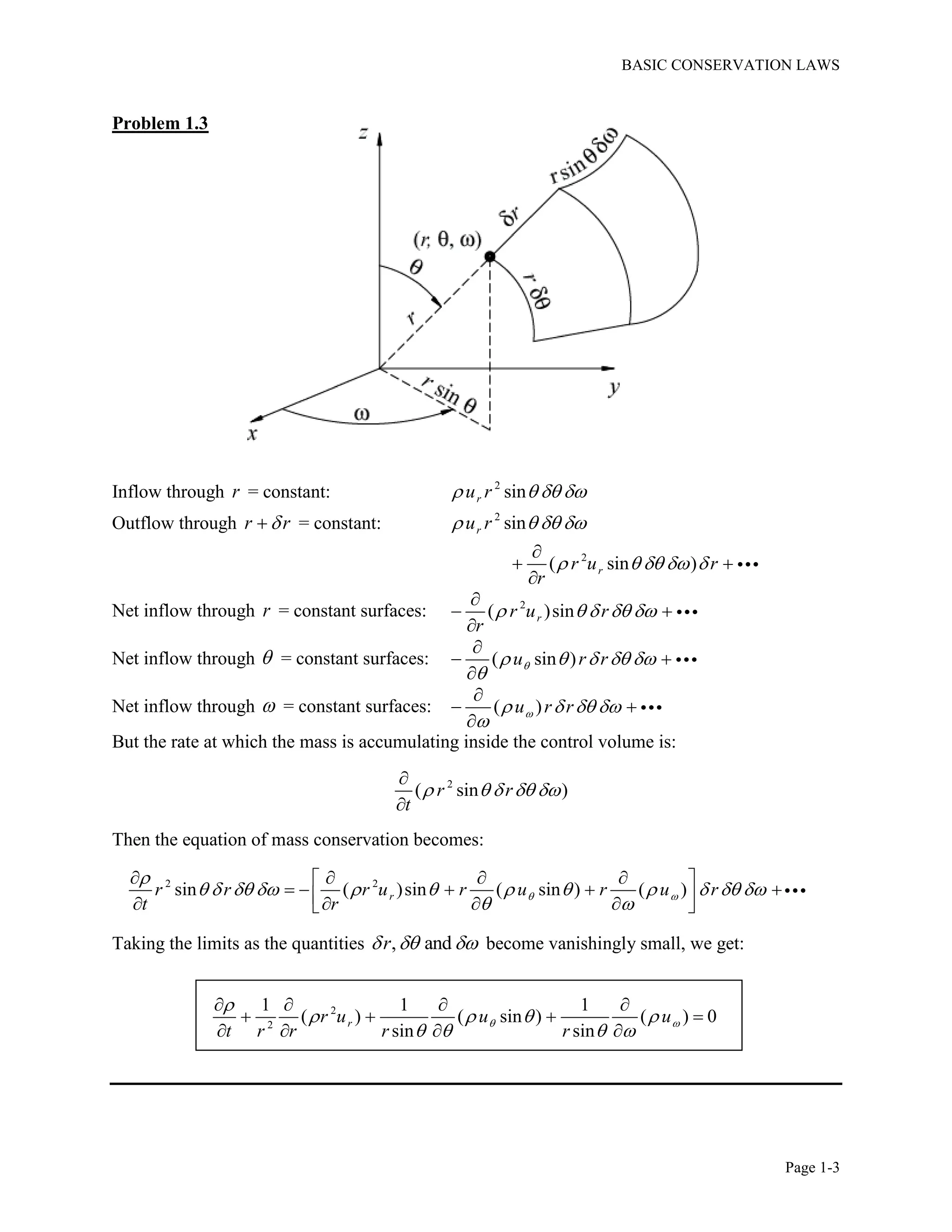
This document contains solutions to problems related to basic conservation laws in fluid mechanics. Specifically: - Problem 1.1 derives the equation of continuity in Cartesian coordinates from the net inflow/outflow of a control volume. - Problems 1.2-1.4 derive the equation of continuity in cylindrical and spherical polar coordinates by applying transformations to the Cartesian form. - Problem 1.5 provides expressions for converting partial derivatives between Cartesian, cylindrical, and spherical coordinate systems, which are needed for applying conservation laws in different frames of reference.


![[Paul lorrain] solutions_manual_for_electromagneti(bookos.org)](https://cdn.slidesharecdn.com/ss_thumbnails/paullorrainsolutionsmanualforelectromagnetibookos-140312211725-phpapp02-thumbnail.jpg?width=640&height=640&fit=bounds)


