The document details a multi-day workshop on spacecraft RF communication, covering topics such as RF signal transmission, modulation techniques (like BPSK and QPSK), telemetry systems, and error control coding. It emphasizes the significance of channel coding for long-distance communication, using examples like the Voyager mission, and discusses various signal processing techniques. Key concepts include Doppler effects, time dilation, link budgets, and advanced decoding methods like turbo decoding.

1. Spacecraft RF Communication
Day 1:
•
•
•
•
Spacecraft communications introduction
RF signal transmission
RF carrier modulation
Noise and link budgets
Day 2:
•
•
•
•
Error control coding
Telemetry systems
Analog Signal Processing
Digital Signal Processing
Day 3:
• Kalman filters
• Satellite systems
• Special topics
10/30/2013
John Reyland, PhD
Stop me
and ask!!!!

2. RF Signal Transmission
Doppler frequency shift and
time dilation affect RF channels
where receiver and/or
transmitter are moving relative
to each other
v(t )
θ (t )
vr (t ) = v(t ) co s(θ (t ) )
Fixed inertial reference frame
10/30/2013
.

3. RF Signal Transmission
Some Definitions:
c = Speed of light, 3e8 meters/second
f c = Carrier frequency (Hz)
θ (t ) = Angle between receiver’s forward velocity and
line of sight between transmitter and receiver
(t ) co s θ (t ) )
vr (t ) v=
(
Velocity of receiver relative to transmitter
f d (t ) = Doppler carrier frequency shift at receiver
Tt (t ) = Transmit symbol time
Tr (t ) = Receive symbol time
10/30/2013

4. RF Signal Transmission
Example 1:
f c = 1 GHz = 1e+9 Hz
v(t )= v=
350 meters/second (constant, approx. Mach 1)
θ (t ) = 0 (constant, worst case for Doppler shift)
vr= v= Velocity of receiver relative to transmitter
v
= d
f d (t ) f= f c  =

c
Tt (t ) = Tt =
(1e9 )
350 10(350)
=
= 1167 Hz Doppler carrier frequency shift at receiver
=
3e8
3
1
= 1e − 6 = Transmit symbol time
1e + 6
Tr (t ) =Tr =Tt +
vTt
 350 
=(1e − 6) 1 +
 =(1e − 6)(1.000001167) = Receive symbol time
c
 3e8 
This means receive symbol time increases by 0.0001167%. - called time dilation
10/30/2013

5. RF Signal Transmission
d = distance between transmitter and receiver at leading edge of transmit pulse
d+vTt = distance between transmitter and receiver at trailing edge of transmit pulse
d
= Propagation time at leading edge of transmit pulse
c
Received Pulse, duration = Tr
 d + vTt
 c


 = Propagation time at trailing edge of transmit pulse

Transmit Pulse, duration = Tt
 d + vTt
 c

Tt +
 d vTt Additional time duration of pulse at the receiver
− c = c =

vTt
 v
= Tt 1 +  = Dilated time duration of pulse at the receiver
c
 c
10/30/2013

6. RF Carrier Modulation
Binary Phase Shift Keying (BPSK)
a ( n)
b( n)
1 ⇒ +1
0 ⇒ −1
R=1 implies one modulating
cycle per symbol. R=2.5 in
this example

 R 
cos  2π l   
 L 

p(k )
Antipodal
Mapping
Pulse
Forming
x(k )
y (l )
Modulator
x(k )
n = 0
0
0
0
1
1
1
1
2
2
2
2
3
3
3
3
4
4
4
4
k = 0
1
2
3
4
5
6
7
8
9
10 11 12 13 14 15 16 17 18 19
-2Fb -Fb
0
Fb
2Fb
y (l )
Fc = -RFb
0
10/30/2013
L
2L
3L
4L
5L
John Reyland, PhD
0
Fc = RFb

7. RF Carrier Modulation

 R 
cos  2π l   
 L 

Quadrature Phase Shift Keying (QPSK)
be (ne )
a ( n)
p(k )

 R 
sin  2π l   
 L 

1 ⇒ +1
0 ⇒ −1
bo (no )
Serial 2
Parallel
p(k )
y (l )
yI (l )
xI (l )
yQ (l )
xQ (l )
Modulator
Pulse
Forming
1
0
a ( n)
n = 0
0
0
0
1
1
1
1
2
2
2
= 0
1
2
3
4
5
6
7
8
9
10 11 12 13 14 15 16 17 18 19 20 21 22 23 24 25 26 27 28 29 30 31 32 33 34 35
n = 0
0
0
0
1
1
1
1
2
2
2
= 0
1
2
3
4
5
6
7
8
9
10 11 12 13 14 15 16 17 18 19 20 21 22 23 24 25 26 27 28 29 30 31 32 33 34 35
xI ( k ) k
xQ ( k ) k
2
2
3
3
3
3
3
3
3
3
4
4
4
4
4
4
4
4
5
5
5
5
5
5
5
5
6
6
6
6
6
6
6
6
7
7
7
7
7
7
7
7
8
8
8
8
8
8
8
8
y I (l )
yQ (l )
0
10/30/2013
L
2L
3L
4L
5L
John Reyland, PhD
6L
7L
8L
9L

8. RF Carrier Modulation
OFDM starts by converting high speed symbols indexed by n at rate 1/Ts
Into parallel blocks indexed by k at rate 1/T = M/Ts
bi ( n ) + jbq ( n )
b(4k )
b(4k + 1)
Each channel now transmits
QPSK symbols at block rate Fs/M
s(4k )
s(4k + 1)
b(4k + 2)
IDFT
In this example, M=4
s(4k + 2)
s(4k + 3)
b(4k + 3)
Channel 3 Symbols
Channel 2 Symbols
Channel 1 Symbols
Channel 0 Symbols
n = 0 1 2 3 4 5 6 7 8 9 10 11 12 
k= 0 0 0 0 1 1 1 1 2 2
10/30/2013
2
2
3

© John Reyland, PhD

9. RF Carrier Modulation
Advantage:
Bit polarity can match
alternating I,Q polarity
Disadvantages:
To detect bits, have to know
where two bit pattern
boundaries are. Even/Odd bits
cannot interchange
Important: This signal has only
one bit of modulo 2π phase
memory, i.e. current phase
transition only depends on
previous phase.
10/30/2013
© John Reyland, PhD

10. Noise and Link Budgets
Important antenna specifications:
• Beamwidth: Angular field of view
• Gain: Increase in power due to directionality
• Sidelobe rejection: Attenuation of signals outside beamwidth
10/30/2013
© John Reyland, PhD

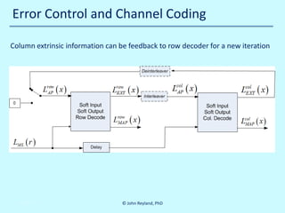
11. Error Control and Channel Coding
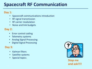
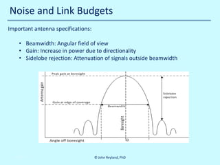
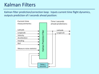
Time Diversity:
After receiver reassembles,
all errors can be corrected
See [R5] and [R6]
10/30/2013
© John Reyland, PhD

12. Error Control and Channel Coding
Maximum Likelihood (ML) detector:
Detection mechanism uses the log-likelihood ratio, for detection
filter output rrec:
 p ( r | S1 ) 
 p1 
= log 
LML = log  
 p (r | S ) 

0 
 p0 

Log-likelihood ratio sign is most probable hard decision
10/30/2013
© John Reyland, PhD

13. Error Control and Channel Coding
ML decisions in a general N dimensional signal space:
1
p ( r | Sm ) =
π N0
N
∏e
−( rk − Smk )
2
N0
k =1
− N0
1
ln p ( r | S=
ln (π N 0 ) −
m)
2
N0
N
∑(r
k =1
k
− S mk )
The most likely transmitted signal Sm
minimizes the Euclidian distance:
D ( r=
, Sm )
10/30/2013
N
∑ ( rk − Smk )
2
k =1
© John Reyland, PhD
2

14. Error Control and Channel Coding
Maximum a posteriori (MAP) detector:
Start with Bayes rule:
p(S | r) =
p (r | S ) p (S )
p (r )
p ( S1 | r )
=
p ( S0 | r )
p ( r | S1 ) p ( S1 )
p (r )
p ( r | S1 ) p ( S1 )
=
p ( r | S0 ) p ( S0 ) p ( r | S0 ) p ( S0 )
p (r )
MAP Log-likelihood ratio = likelihood ratio based on observation + a priori information ratio
LMAP
 p ( S1 | r ) 
 p ( r | S1 ) 
 p ( S1 ) 
log 
= log 
 p(S | r) 

 p ( r | S )  + log  p ( S ) 



0
0 
0 




A priori: Information knowable independent of experience
A posteriori: Information knowable on the basis of experience
10/30/2013
© John Reyland, PhD
LMAP = LML
if p ( S1 ) = p ( S0 )

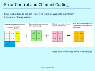
15. Error Control and Channel Coding
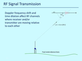
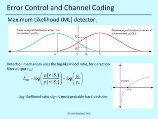
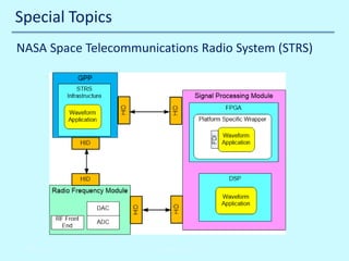
Concatenated coding for Voyager mission to Saturn and Uranus
Power efficiency is extremely important: Coding gain of 6dB can double the
communications range between spacecraft and earth ([C8], page 172)
Voyager telecommunications achieved 10-6 BER at EbN0 = 2.53dB, 2Mbits/sec.
What system considerations are not very important?
Bandwidth efficiency, not many other users out there.
Delay, waiting time for image reconstructions is OK
10/30/2013
© John Reyland, PhD

16. Error Control and Channel Coding
Turbo coding basic concept explained by an example
10/30/2013
© John Reyland, PhD

17. Error Control and Channel Coding
Turbo Decoder diagram for this example:
The maximum a posteriori (MAP) log likelihood ratio:
col
MAP
L
 p ( S1 | r ) 
 p ( r | S1 ) 
 p ( S1 ) 
col
row
= log 
 = log 
 + log 
 = LML + LAP = LML + LEXT
 p(S | r) 
 p (r | S ) 
 p(S ) 
0
0 
0 




10/30/2013
© John Reyland, PhD

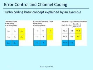
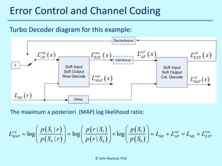
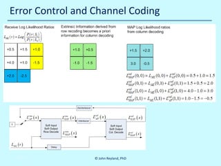
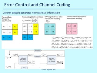
18. Error Control and Channel Coding
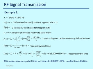
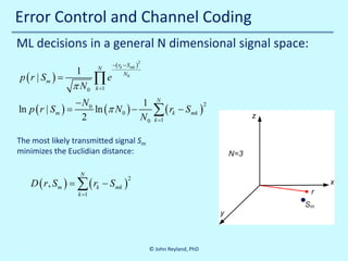
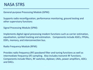
Log likelihood ratio of modulo two addition of two soft decisions (see []):
(
L ( r0 ⊕ r1 ) L ( r0= sig nL ( r0 ) ) sig nL ( r1 ) ) min L ( r0 ) , L ( r1 )
=
)  L ( r1 )
(
(
)
This addition rule is used to combine data and parity into extrinsic information
Extrinsic means extra, or indirect, information derived from the decoding process
10/30/2013
© John Reyland, PhD

19. Error Control and Channel Coding
10/30/2013
© John Reyland, PhD

20. Error Control and Channel Coding
Column decode generates new extrinsic information
10/30/2013
© John Reyland, PhD

21. Error Control and Channel Coding
Column extrinsic information can be feedback to row decoder for a new iteration
10/30/2013
© John Reyland, PhD

22. Error Control and Channel Coding
Final turbo decode output is derived from all available statistically
independent information:
Note how confidence levels are improved
10/30/2013
© John Reyland, PhD

23. Channel Equalization Techniques
Raised cosine pulses have an extremely important attribute: at the ideal
sampling points, they don’t interfere with each other
Over an ideal channel, delayed transmit signal will be observed at the receiver.
Ideal channel:
10/30/2013
sreceived (t ) stransmit (t − δ )
=
John Reyland, PhD

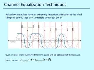
24. Channel Equalization Techniques
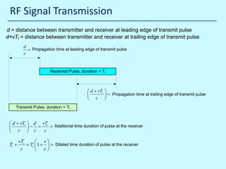
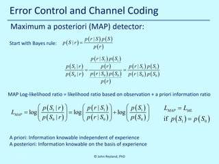
A decision feedback
nonlinear adaptive
equalizer:
See [E1] and [E2]
10/30/2013
© John Reyland, PhD

25. Analog Signal Processing
For gain planning, receiver has to cope with contradicting requirements
ADC Input: Only one optimum power level for best performance
= Max ADC input – received signal peak to average power ratio (PAPPR)
Antenna Input: Needs to handle wide range of inputs from
-100 dBm or less to 0dBm or more
dBm
  P10  


Pwatts 



PdBm 10log10 
Pwatts
= 0.001  10




 0.001 


10
0.1
−100dBm ⇒ 10−1010−3 =−13 = picowatt
0dBm ⇒ 1milliwatt
10/30/2013
© John Reyland, PhD

26. Analog Signal Processing
A complex representation is required at baseband because the modulation will
cause the instantaneous phase to go positive or negation:
= co s θ BB (t ) ) + j sin (θ BB (t ) )
e jθ BB (t )
(
Because the phase is now always positive, complex exponential terms are redundant
e
= co s ωRF t + θ BB (t ) ) + j sin (ωRF t + θ BB (t ) )
(
j (ωRF t +θ BB ( t ) )
Signal now can be real:
cos (ωRF t + θ BB (t= e
))
j (ωRF t +θ BB ( t ) )
+e
− j (ωRF t +θ BB ( t ) )
This forces the existence of a negative image (ignored for most analog processing):
10/30/2013
© John Reyland, PhD

27. Analog Signal Processing
Voltage Sampling: Undesired signals are all aliased at full power:
Current Sampling: Images at multiples of sampling rate are attenuated:
10/30/2013
© John Reyland, PhD

28. Analog Signal Processing
Compete Transmitter
Let’s discuss the function of the reconstruction filter and the bandpass filter…
10/30/2013
© John Reyland, PhD

29. Digital Signal Processing
We will organize our DSP discussion around the digital receiver architecture below:
This setup is suitable for many linear modulations. Nonlinear demodulation would
replace the equalizer with a phase discriminator and also probably not have carrier
tracking.
10/30/2013
John Reyland, PhD

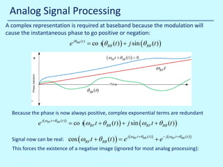
30. Digital Signal Processing
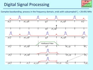
Intermediate center frequency Fif = 44.2368 MHz.
Does this mean sampling frequency Fs > 88.4736 MHz ?
No, we can bandpass sample, by making Fs = (4/3) Fif = 58.9824 MHz. This has advantages:
• Lower sample rate => smaller sample buffers and fewer FPGA timing problems
• Fif can be higher for the same sample rate, this may make frequency planning easier
Disadvantage is that noise in the range [Fs/2 Fs] is folded back into [0 Fs/2]
10/30/2013
John Reyland, PhD

31. Digital Signal Processing
Complex basebanding process in the frequency domain, ends with subsampled Fs = 29.491 MHz
10/30/2013
John Reyland, PhD

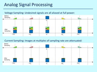
32. Digital Signal Processing
Halfband Filter response
HalfBand filter Impulse Response, Order=11
0.6
0.4
Typical Matlab code:
0.2
0
-0.2
Fss = 58.9824e6;
1
2
3
4
5
6
7
8
9
10
11
Resp, dB
0
-10
-20
-30
-40
0
3.6864
7.3728
11.0592 14.7456 18.432
Frequency (MHz)
22.1184 25.8048 29.4912
0
3.6864
7.3728
11.0592 14.7456 18.432
Frequency (MHz)
22.1184 25.8048 29.4912
Resp, linear
1
0.5
0
10/30/2013
John Reyland, PhD
% Setup halfband filter for input subsampling
PassBandEdge = 1/2-1/8;
StopBandRipple = 0.1;
b=firhalfband('minorder', …
PassBandEdge, …
StopBandRipple, …
'kaiser');
% Check frequency response
[hb,wb] = freqz(b,1,2048);
plot(wb,10*log10(abs(hb)));
set(gca,'XLim',[0 pi]);
set(gca,'XTick',0:pi/8:pi);
set(gca,'XTickLabel',(0:(Fss/16):(Fss/2))/1e6);

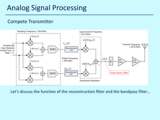
33. Digital Signal Processing
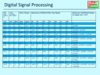
DSP Circuits for IF to Complex BB process
Fs/4 Local Oscillator
Inphase Halfband Filter
I(n) + jQ(n) = [1+j0,0+j1,-1+j0,0-j1,1+j0, ...]
HI(z) = h0 + z-2h2 + z-3h3 + z-4h4 + z-6h6
Ib(n)
x(n)
Z-1
h0
Z-1
Z-1
Z-1
Z-1
Z-1
0
h2
h3
h4
0
h6
Ihb(n)
2
Qb(n)
Z-1
h0
Z-1
Z-1
Z-1
Z-1
Z-1
0
h2
h3
h4
0
h6
Qhb(n)
2
Quadrature Halfband Filter
HQ(z) = h0 + z-2h2 + z-3h3 + z-4h4 + z-6h6
10/30/2013
John Reyland, PhD

34. Digital Signal Processing
Input
Samp.
Index @
Fs
Local
Oscillator:
I(n) + jQ(n) =
Mixer Output
Quadrature Halfband Filter Tap Signals
x(n)
x(0)
x(1)
x(2)
x(3)
x(4)
x(5)
x(6)
x(7)
I(n)
1
0
-1
0
1
0
-1
0
Q(n)
0
1
0
-1
0
1
0
-1
Ib(n)
x(0)
0
-x(2)
0
x(4)
0
-x(6)
0
Qb(n)
0
x(1)
0
-x(3)
0
x(5)
0
-x(7)
h0
0
x(1)
0
-x(3)
0
x(5)
0
-x(7)
0
0
0
x(1)
0
-x(3)
0
x(5)
0
h2
0
0
0
x(1)
0
-x(3)
0
x(5)
h3
0
0
0
0
x(1)
0
-x(3)
0
h4
0
0
0
0
0
x(1)
0
-x(3)
0
0
0
0
0
0
0
x(1)
0
h6
0
0
0
0
0
0
0
x(1)
x(8)
x(9)
1
0
0
1
x(8)
0
0
x(9)
0
x(9)
-x(7)
0
0
-x(7)
x(5)
0
0
x(5)
-x(3)
0
0
-x(3)
x(10)
x(11)
-1
0
0
-1
-x(10)
0
0
-x(11)
0
-x(11)
x(9)
0
0
x(9)
-x(7)
0
0
-x(7)
x(5)
0
0
x(5)
x(12)
x(13)
1
0
0
1
x(12)
0
0
x(13)
0
x(13)
-x(11)
0
0
-x(11)
x(9)
0
0
x(9)
-x(7)
0
0
-x(7)
x(14)
x(15)
-1
0
0
-1
-x(14)
0
0
-x(15)
0
-x(15)
x(13)
0
0
x(13)
-x(11)
0
0
-x(11)
x(9)
0
0
x(9)
10/30/2013
John Reyland, PhD
Quadrature Half Band Output
@ sample rate = Fs/2
0
x(1)*h0
0
-x(3)*h0 + x(1)*h2
x(1)*h3
x(5)*h0 - x(3)*h2 + x(1)*h4
-x(3)*h3
-x(7)*h0 + x(5)*h2 - x(3)*h4 +
x(1)*h6
x(5)*h3
x(9)*h0 - x(7)*h2 + x(5)*h4 x(3)*h6
-x(7)*h3
-x(11)*h0 + x(9)*h2 - x(7)*h4 +
x(5)*h6
x(9)*h3
x(13)*h0 - x(11)*h2 + x(9)*h4 x(7)*h6
-x(11)*h3
-x(15)*h0 + x(13)*h2 - x(11)*h4
+ x(9)*h6

35. Spacecraft Downlink Tracking
Downlink Doppler measurements: Range rate and uplink pre-compensation
10/30/2013
John Reyland, PhD

36. Kalman Filters
A Kalman filter estimates the state of an ‘n’ dimensional discrete time process
governed by the linear stochastic difference equation:
x(k ) Ax(k − 1) + Bu (k − 1) + w(k − 1)
=
A = (n by n)
Represents the system dynamics of the system whose state we
are trying to estimate. Control input matrix B = (n by l) is optional
Discrete time state vector
x(k )
is not directly observable, however we can measure:
= Hx(k ) + v(k )
z (k )
H = (m by n)
v(k ) is a random variable representing the normally distributed measurement noise
p (v) ~ N ( 0, Q )
w(k )
is a random variable representing the normally distributed process noise
p ( w) ~ N ( 0, Q )
10/30/2013
John Reyland, PhD

37. Kalman Filters
Kalman filter prediction/correction loop: Inputs current time flight dynamics,
outputs prediction of t seconds ahead position:
10/30/2013
John Reyland, PhD

38. Special Topics
NASA Space Telecommunications Radio System (STRS)
10/30/2013
John Reyland, PhD

39. NASA STRS
General-purpose Processing Module (GPM):
Supports radio reconfiguration, performance monitoring, ground testing and
other supervisory functions
Signal Processing Module (SPM):
Implements digital signal processing modem functions such as carrier estimation,
equalization, symbol tracking and estimation. Components include ASICs, FPGAs,
DSPs, memory, and interconnection bus.
Radio Frequency Module (RFM):
Provides radio frequency (RF) passband filter and tuning functions as well as
intermediate frequency (IF) sampling. Also includes transmit RF functions.
Components include filters, RF switches, diplexer, LNAs, power amplifiers, ADCs
and DACs.
10/30/2013
John Reyland, PhD