Signal Processing

1
Signal Processing
Shayan Hosseinpouli
Khashayar Goshtasbi
EE113
UCLA
Professor Daneshrad
16 June 2017

2
Abstract
Project was to generate sinusoid signals at different frequencies and observe their
sound and frequency response. Low and High pass filters were designed to eliminate the
unwanted frequency. A nonlinear function with a goal of clipping the amplitude at 50%
was designed and analyzed in time and frequency domain. Matlab was used for all
purposes of this project to understand applications of topics we studied this quarter. The
goal of this project is to get hands-on experience with Digital Signal Processing and get
familiar with Matlab usage. Matlab is electronic design automation. It is one of the most
powerful sources in the Signal Processing world as it allows to simulate signals, process,
and analyze them.
Theory
Continues time domain signals are analog signals. To be processed they need to
be digitized, hence, sampled at a certain sampling frequency. In all the steps, Fs=5 kHz
was used. For sampling to perform properly aliasing should not occur. Nyquist theorem
provides a lower bound on how small Fs can be so that we can recover the original signal
x(t) from the sampled version x(n). For the two tones of 400 and 1500 Hz here the
Nyquist rate is 3 kHz.
As the signals are sampled we arrive at the discrete time domain. Frequency responses
are obtained by taking the DTFT of sampled signals. Matlab obtains frequency responses
by taking FFT of signals. FFT is an efficient way to obtain DFT of a signal. DFT is a
subset of DTFT where:
X(k) = X(ejw
)|w=2πk/N
Through all steps signals were generated for 5 seconds. For T = 5s , Fs = 5 kHz, N was
taken to be N = T*Fs = 25000. Through all steps 25k point FFT was taken. In all steps
magnitude responses have been normalized by dividing the magnitude response by N.
Electronic filters are circuits that perform signal processing functions to annihilate
unwanted frequency components from the signal and or enhance certain ones. Filters are
modeled mathematically to analyze their impulse and frequency responses.

3
Step 1
For the first part of this project, we generated a 400 Hz sine wave vector of duration 5
seconds, and then we sampled this generated signal at a sampling frequency of Fs =5
KHz.
Ts = 1/Fs
Tone1_dig = sin(2*pi*400*n*Ts)
And then we played the tone out of our computer and listened to it to see how the signal
sounds just by itself, and then we generated a second tone of 1.5 KHz of duration 5
seconds, which was sampled at a frequency of 5 KHz.
Once both the signals were generated, we added the two tones together and played the
results from our computer and listened to it.
Tone12_dig = Tone1_dig +Tone2_dig
Tone12_dig = sin(2*pi*400*n*Ts) + sin(2*pi*1500*n*Ts)
The sound of tone2_dig had a higher pitch than the sound of tone1_dig because of the
higher frequency. Sound of tone12_dig seemed as the sound both tones superimposed.
• Figure 1: Tone12_dig = sin(2*pi*400*n*Ts) + sin(2*pi*1500*n*Ts)

4
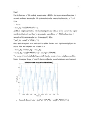
For T = 5s , Fs = 5 kHz, N was taken to be N = T*Fs = 25000.
25000 point FFT of Tone12_dig was taken.
FFT{Tone1_dig} + FFT{Tone2)dig} = FFT{Tone12_dig} because of linearity property
of FFT.
FFT{Tone12_dig} = jN/2*[-δ(k – 400) + δ(k – (N – 400) - δ(k – 1500) + δ(k – (N – 1500)]
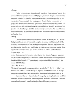
Furthermore, FFT{Tone12_dig} was divided by N to obtain a normalized magnitude
response in the frequency domain.
FFT of a signal is periodic with N. FFT{Tone12}, implies there should impulses with
magnitude of 0.5 at ±400 Hz and ±1500 Hz in the frequency domain. Theory confirms
the following Matlab graph.
- Figure 2: FFT of the added tones.
-2500 -2000 -1500 -1000 -500 0 500 1000 1500 2000 2500
Frequency [Hz]
0
0.1
0.2
0.3
0.4
0.5
0.6
0.7
0.8
0.9
1
NormalizedMagnitude
FFT of Added Tones (Magnitude)

5
- Figure 3: Phase Response for FFT of the added tones.
Matlab computes and plots the FFT through numerical calculations. Result is we have
points with infinitesimal magnitudes that should have been zero in theory. Those
infinitesimal magnitudes have non-zero phase that explains the messy phase graph in
figure 3. In theory, for FFT{Tone12_dig} phase response has to be -π/2 at 400 and 1500
Hz for the term –j and π/2 at -400 and -1500 Hz for the term j.
Step 2
Theory
Low pass filter (LPF) is a filter that passes the signals with frequencies lower than
a certain cutoff frequency and attenuates the signals with frequencies higher than the
cutoff frequency. Low pass filters are used to clean up signals, remove noise, perform
data averaging, and discover important pattern through the generated signals.
An ideal low pass filter is an LTI system whose frequency response is assumed to
be of the general form:
Where 0 < wc < π is called the cutoff frequency and k0 is an integer. The
magnitude response of the ideal low pass filter is constant and equal to A over
-2500 -2498 -2496 -2494 -2492 -2490 -2488 -2486 -2484 -2482 -2480
Frequency [Hz]
-4
-3
-2
-1
0
1
2
3
4
Phase[rad]
Phase of FFT of Added Tones Snippet

6
the interval [-wc,wc], while the phase response is linear over the same interval
with its slope dictated by the value of k0. The range of frequencies [-wc,wc] is
called the passband region, and the interval over which the magnitude of the
frequency response is zero called the stopband region. Frequency response of the
ideal lowpass filter is illustrated below. (Sayed 447)
- Figure 4: Magnitude and phase responses of an ideal low pass filter.
Ideal filters are also called “brick wall” filters because of the way they look.
Impulse response of an ideal LPF is in the form of a sinc function as:
DTFT{wc/π * sinc(wcn)} = rect(
!
"!#
) where wc is the cutoff frequency.
The following circuit is the simplest form of an RC low pass filter with a transfer
function of: |Vout/Vin| =
$
$ & '()*
For this RC circuit as w approaches high frequencies, the transfer function’s value
decreases, approaching zero. The cutoff frequency can be tailored by assigning different
values to R or C.

7
- figure 5: simple RC low pass filter.
Design
There are:
Tone12_dig= sin(2*pi*400*n*Ts) + sin(2*pi*1500*n*Ts).
Goal of this step is to have a filter that passes the 400 Hz tone and suppresses the 1500
Hz tone.
A sinc function was chose to model a LPF.
For Tone1_dig: f1sampled = 2*pi*400*Ts = 0.16π rad
For Tone1_dig: f2sampled = 2*pi*1500*Ts = 0.6π rad
For f2sampled to be suppressed: wc < 0.6π, Let wc,LPF = π/3. LPF for step 2 was designed as:
sincfilter = 1/3 sinc(π/3n) ; length =10
The latter is an IIR filter as the sinc function goes to infinity in positive and negative
regions. An ideal sinc filter has infinite terms in its impulse response and hence in its Z-
transform. There are infinitely many poles and zeros in the Z-transform of the ideal sinc
filter. As for the truncated sinc filter designed here, the number of poles and zeros are
limited. For the LPF, zeros are placed after the cutoff frequency wc=π/3 to zero out the
stopband frequencies. Poles are before the wc=π/3 to enhance the passage of passband
frequencies.
DTFT{1/3 sinc(π/3n)} = rect(
(
"+/-
). rect(
(
"+/-
), is a brick wall filter with magnitude
response of the shape in figure 4 with wc=π/3.
In time domain, filtering corresponds to convolution of the signal with filter in time
domain. Convolution in time domain corresponds to multiplication in frequency domain.

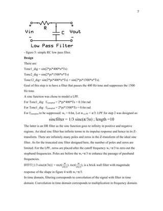
8
As the magnitude response for the designed LPF is zero for π/3<w<π , f2sampled = 0.6π will
be suppressed; 1500 Hz tone will be suppressed.
Impulse response of the desgined LPF is illustrated below.
-
- Figure 6: impulse response of designed LPF 1/3 sinc(π/3n).
Note that this filter was designed with a length of 10 points for n∈ [-5:5]. It satisfies the
requirements and has a low cost.
As DTFT{1/3 sinc(π/3n)} = rect(
(
"+/-
), the magnitude and phase responses of the LPF is
illustrated below.
-1 -0.8 -0.6 -0.4 -0.2 0 0.2 0.4 0.6 0.8 1
Time [s] #10-3
-0.1
-0.05
0
0.05
0.1
0.15
0.2
0.25
0.3
0.35
Amplitude
Filter Impulse Response

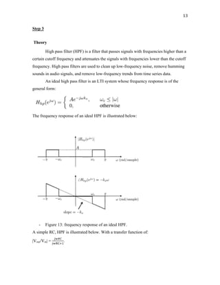
9
- figure 7: magnitude and phase response of LPF.
Performance of the filter increases as a function of the length. Complexity of the filter
increases with the length as the number of add/multiply operation to realize the filter
increase. Hence, cost of the filter increases with the length. Designing filters, one has
to keep in mind the requirements and the cost filter shall have. High performance
filters have a high roll-off. Roll-off is the steepness of the magnitude response in the
transition region between passband and stopband. Decreasing length decreases roll-
off. To optimize performance and cost, different cutoff frequencies were trialed.
Wc=π/3 was found to be at a location that would result in enough attenuation of the
1500 Hz tone while keeping the cost low.
In theory for an ideal filter the magnitude response is zero for wc<w<π therefore,
frequencies in the stopband will be eliminated.
In practice we expect an annihilation of minimum 20dB for the 1500 Hz tone.
-4 -3 -2 -1 0 1 2 3
Omega [rad/sample]
0
0.2
0.4
0.6
0.8
1
1.2
Magnitude
Low Pass Filter
-4 -3 -2 -1 0 1 2 3
Omega [rad/sample]
-3
-2
-1
0
1
2
3
Phase[rad]
Low Pass Filter

10
- Figure 8: output of the LPF.
Note the ±1500 Hz tones are annihilated. Following is the magnitude response for the
output in a decibel scale to assert the 20dB annihilation.
- Figure 9: magnitude response for output in dB scale.
Note that the ± 1500 Hz tones are annihilated by about 100 dB.
Output in the time domain is convolution of the signal with the sincfilter.
Output (time domain) = conv(tone12_dig, sincfilter)
-2500 -2000 -1500 -1000 -500 0 500 1000 1500 2000 2500
Frequency [Hz]
0
0.2
0.4
0.6
0.8
1
NormalizedMagnitude
Output of Filter (Frequency Domain)
-2500 -2000 -1500 -1000 -500 0 500 1000 1500 2000 2500
Frequency [Hz]
-3
-2
-1
0
1
2
3
Phase[rad]
Phase of Output of Filter
-2500 -2000 -1500 -1000 -500 0 500 1000 1500 2000 2500
Frequency [Hz]
-250
-200
-150
-100
-50
0
NormalizedMagnitude[dB]
Output of Filter (dB Scale)

11
- Figure 10: output of LPF in time domain.
The time domain output was very dense for the duration of 5 seconds. The snippets for
left and right sides illustrate a convolution graph as expected. Graphically, convolution
with the sinc function has an enveloping effect which is observed at the very left of “left
side snippet” in figure 10 and through out both snippets for the time domain output in
figure 10.
Discussion
There were tradeoffs arriving at this filter. To keep the cost low the filter is far
from looking ideal. That decreases the performance as discussed earlier. By finding the
right cutoff frequency, we were able to satisfy the requirements and keep the cost low as
our filter is realized for only 10 points.
This is how a high performance high cost version of the same filter would look like.
Increasing the length makes the filter approach the brick wall shape.
0 1 2 3 4 5
Time [s]
-1.5
-1
-0.5
0
0.5
1
1.5
Amplitude
Output of Filter (Time Domain)
0 0.02 0.04 0.06
Time [s]
-1.5
-1
-0.5
0
0.5
1
1.5
Amplitude
Output of Filter Left Side Snippet
4.94 4.96 4.98 5
Time [s]
-1.5
-1
-0.5
0
0.5
1
1.5
Amplitude
Output of Filter Right Side Snippet

12
- Figure 11: high cost, high performance LPF.
Choosing the right frequency is important while keeping the cost low. Observe how
magnitude response would look for wc=π/2.
- Figure 12: magnitude response for filter output for wc=π/2.
The 1500 Hz tone is not as much annihilated as wc=π/3 case and also there is suppression
for 400 Hz tone.
-4 -3 -2 -1 0 1 2 3 4
Omega [rad/sample]
0
0.2
0.4
0.6
0.8
1
1.2
Magnitude
Low Pass Filter
-4 -3 -2 -1 0 1 2 3 4
Omega [rad/sample]
-4
-2
0
2
4
Phase[rad]
Low Pass Filter
-2500 -2000 -1500 -1000 -500 0 500 1000 1500 2000 2500
Frequency [Hz]
-300
-250
-200
-150
-100
-50
0
Output of Filter (dB Scale)

13
Step 3
Theory
High pass filter (HPF) is a filter that passes signals with frequencies higher than a
certain cutoff frequency and attenuates the signals with frequencies lower than the cutoff
frequency. High pass filters are used to clean up low-frequency noise, remove humming
sounds in audio signals, and remove low-frequency trends from time series data.
An ideal high pass filter is an LTI system whose frequency response is of the
general form:
The frequency response of an ideal HPF is illustrated below:
- Figure 13: frequency response of an ideal HPF.
A simple RC, HPF is illustrated below. With a transfer function of:
|Vout/Vin| =
.!/0
'()*&$
.

14
For this RC circuit as w approaches low frequencies, transfer function’s value decreases,
approaching zero. The circuit can be tailored by assigning different values to R or C.
- Figure 14: simple RC HPF
Design
There is the signal of:
Tone12_dig = sin(2*pi*400*n*Ts) + sin(2*pi*1500*n*Ts).
Goal of this step is to have a filter that passes the 1500 Hz tone and suppresses the 400
Hz tone.
HPF was designed in the time domain using a sinc function multiplied by a cosine.
Multiplication in the time domain corresponds to convolution in the frequency domain.
DTFT{cos(w0n)} = π[δ(w-w0)+δ(w+w0)]
Convolution with δ(w±w0) results in delays for frequency response of the original
function by ±w0.
HPF was designed with a cutoff frequency of wc=6π/11 rad as:
Sincfilter = cos(πn)*(6/11)*sinc(
1+
$$
n) ; length =10
The latter is an IIR filter as the sinc function has goes to infinity in positive and negative
time. The passband region for the HPF is for w∈[6π/11,π]. Stopband region is for
w∈[0,6π/11). An ideal sinc filter has infinite terms in its impulse response and hence in
its Z-transform. There would be infinitely many poles and zeros in the Z-transform of the
ideal sinc filter. As for the truncated sinc filter designed here, the number of poles and
zeros are limited. For the HPF, zeros are placed before the cutoff frequency wc = 6π/11 to
zero out the stopband frequencies. Poles are after wc = 6π/11 to enhance the passage of
passband frequencies.

15
Multiplication by the cosine shifts the frequency response of sinc(
1+
$$
n) by ±π.
It is expected for signals with frequencies 0<w <6π/11 to be eliminated. This particular
wc=6π/11 was chosen because it satisfied the requirements and kept the cost low with a
length of 10 points. It was found by iteration though different cutoff frequencies. the
frequency to be passed here is 1500 Hz corresponding to:
f2sampled = 0.6π rad.
Keeping the cost low results in a far from ideal looking filter. It would look smoother
than a brick wall filter and with a smaller roll-off. Hence, the cutoff frequency needs to
be pushed closer to the passing frequency. Note, f2sampled = 6π/10 rad and wc=6π/11 rad.
You don’t want to get too close because the frequency to be passed would start getting
suppressed as well. The equilibrium is to be found.
As Sincfilter = cos(πn)*(6/11)*sinc(
1+
$$
n), the impulse response is a truncated sinc
function.
- Figure 15: impulse response of HPF = cos(πn)*(6/11)*sinc(
1+
$$
n)
-1 -0.8 -0.6 -0.4 -0.2 0 0.2 0.4 0.6 0.8 1
Time [s] #10-3
-0.4
-0.3
-0.2
-0.1
0
0.1
0.2
0.3
0.4
0.5
0.6
Amplitude
Filter Impulse Response

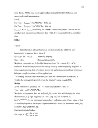
16
As DTFT{cos(πn)*(6/11)*sinc(
1+
$$
n)}=0.5rect(
(3+
$"+/$$
) + 0.5rect(
(&+
$"+/$$
), magnitude
and phase responses of the HPF is illustrated below.
- Figure 16: Magnitude and phase response of the HPF.
Note that the filter was realized for 10 points for n∈[-5:5] to reduce complexity thus the
number of multiply/add operations to realize the filter.
In theory for an ideal filter the magnitude response is zero for 0<w<wc therefore,
frequencies in the stopband will be eliminated. In practice we expect an annihilation of
minimum 30dB for the 400 Hz tone.
-4 -3 -2 -1 0 1 2 3
Omega [rad/sample]
0
0.2
0.4
0.6
0.8
1
1.2
Magnitude High Pass Filter Magnitude
-4 -3 -2 -1 0 1 2 3
Omega [rad/sample]
-3
-2
-1
0
1
2
3
Phase[rad]
High Pass Filter Phase

17
- Figure 17: magnitude and phase response for output of the LPF.
Note the ±400 Hz tones are annihilated. Following is the magnitude response for the
output in a decibel scale to assert the 30dB annihilation.
- Figure 18: magnitude response for output of HPF in dB scale.
Note that the ± 400 Hz tones are annihilated by about 120 dB.
Output in the time domain is convolution of the signal with the sincfilter.
Output (time domain) = conv(tone12_dig, sincfilter)
-2500 -2000 -1500 -1000 -500 0 500 1000 1500 2000 2500
Frequency [Hz]
0
0.2
0.4
0.6
0.8
1
NormalizedMagnitude
Output of Filter (f domain, Magnitude)
-2500 -2000 -1500 -1000 -500 0 500 1000 1500 2000 2500
Frequency [Hz]
-4
-2
0
2
4
Phase[rad]
Output of Filter (f domain, Phase)
-2500 -2000 -1500 -1000 -500 0 500 1000 1500 2000 2500
Frequency [Hz]
-250
-200
-150
-100
-50
0
Output of Filter (f domain, Magnitude in dB scale)

18
- figure 20: output of HPF in time domain.
The time domain output was very dense for the duration of 5 seconds. The snippets for
the left and right sides illustrates a convolution graph as expected. Graphically,
convolution with sinc function has an enveloping effect which is observed at the very left
of “left side snippet” in figure 20 and through out both snippets for time domain output in
figure 20.
Discussion
There were tradeoffs arriving at this filter. To keep the cost low the filter is far
from looking ideal. That decreases the performance as discussed earlier in step 2. By
finding the right cutoff frequency, we were able to satisfy the requirements and keep the
cost low as the filter is realized for only 10 points. In the HPF case wc was found by
getting as close as possible to the passing frequency but not so close that it would
annihilate the passing frequency.
This is how a high performance high cost version of the same filter would look.
Increasing the length makes the filter approach the brick wall shape.
0 1 2 3 4 5
Time [s]
-1.5
-1
-0.5
0
0.5
1
1.5
Amplitude
Output of Filter (Time Domain)
0 0.01 0.02 0.03 0.04
Time [s]
-1.5
-1
-0.5
0
0.5
1
1.5
Amplitude
Output of Filter left Side Snippet
4.96 4.97 4.98 4.99 5 5.01
Time [s]
-1.5
-1
-0.5
0
0.5
1
1.5
Amplitude
Output of Filter Right Side Snippet

19
- Figure 21: high cost, high performance HPF.
Note the brick wall look in figure 21.
Choosing the right frequency is important while keeping the cost low. Observe how
magnitude response would look for wc=π/3.
- Figure 22: magnitude response for filter output for wc=π/3.
-4 -3 -2 -1 0 1 2 3 4
Omega [rad/sample]
0
0.2
0.4
0.6
0.8
1
1.2
Magnitude
High Pass Filter Magnitude
-4 -3 -2 -1 0 1 2 3 4
Omega [rad/sample]
-3
-2
-1
0
1
2
3
Phase[rad]
High Pass Filter Phase
-2500 -2000 -1500 -1000 -500 0 500 1000 1500 2000 2500
Frequency [Hz]
-300
-250
-200
-150
-100
-50
Output of Filter (f domain, Magnitude in dB scale)

20
Note that the 400 Hz tone is not suppressed as much and the 1500 Hz tone is also
suppressed which is undesirable.
Recall:
For Tone1: f1sampled = 2*pi*400*Ts = 0.16π rad
For Tone1: f2sampled = 2*pi*1500*Ts = 0.6π rad
f1sampled < π/3 < f2sampled technically, the 1500 Hz should have passed. This was not the
case here as it was suppressed by more than 50 dB. It is because of the low cost of the
filter.
Step 4
Theory
In mathematics, a linear function is one that satisfies the additivity and
homogeneity properties. f(x) is linear if:
f(x1+x2) = f(x1) + f(x2) Additivity property
f(αx) = αf(x) Homogeneity property
Nonlinear systems are not defined by linear functions. For example, f(x) = x2
is
nonlinear. A nonlinear system does not satisfy additivty and homogeneity properties in
input/output mapping. Lots of systems for real life applications are nonlinear one reason
being the complexity of the real life applications.
The clipping function here is nonlinear, as it does not let the output exceed 50%. It
violates the homogeneity property when the function’s value exceeds 50%.
Design
A 400 Hz tone was generated for T = 5 s and sampled at Fs= 5 kHz as:
We desire an output that does not let Tone1_dig exceed 50% while keeping the other
characteristics, e.g. sign, frequency, of Tone1_dig. x(n) can be written as
|x(n)|*ej*phase(x(n))
. As our sine vector here produces real values only, it has a phase of 0 or
±π resulting in positive and negative signs respectively. Hence, let’s consider Tone1_dig
as |Tone1_dig|*sgn(Tone1_dg).
Sign function is defined as:
f(n) = sgn(n) =
−1 for n < 0
+1 for n > 0

21
For the amplitude, the 50% clipping can be done by taking the minimum of |Tone1_dig|
and 0.50.
The clipping function was designed as:
y = sgn(tone1_dig).*min(abs(tone1_dig), .5)
Discussion
The time domain output of clipping function is illustrated below.
- Figure 23: time domain output of the clipping function.
Figure illustrates Tone1_dig = sin(2*pi*400*n*Ts) clipped at 50%.
Signals can be written as their Fourier series expansion. The square-wave-looking output
of the clipping function is a summation of sinusoids at integer multiples of the
fundamental frequency of. As Tone1_dig = sin(2*pi*400*n*Ts), the fundamental
frequency is f0 = 400 Hz. We expect frequency response at frequencies equal to kf0 where
k is an integer.
kf0 = ±400, ±800, ±1200, ±1600, ±2000, ±2400, ±2800 …
fn = kf0 is called the nth
harmonic. Note that we are sampling the 400 Hz tone at 5kHz. At
the 6th
harmonic (f6=2800 Hz) and beyond there will be aliasing as the Nyquist rate
exceeds 5kHz.
0 0.002 0.004 0.006 0.008 0.01 0.012 0.014 0.016 0.018 0.02
Time [s]
-1
-0.8
-0.6
-0.4
-0.2
0
0.2
0.4
0.6
0.8
1
Amplitude
Output of Clipping Function Snippet (time domain)

22
Following is the frequency response for output of the clipping function.
- Figure 24: frequency response for output of clipping function.
As Tone1_dig = sin(2*pi*400*n*Ts), the fundamental frequency is f0 = 400 Hz.
In the magnitude response we observe responses at ±400, ±800, ±1200 and ±2000. There
are also different magnitudes in the magnitude response. The magnitude response at ±400
Hz is not 0.5 because it has been clipped in time domain. It would have been 0.5 should
the signal went all the way to 1. As for magnitude responses at the other harmonics, they
are not equal because the Fourier coefficients at those harmonics are not equal. There is
also magnitude response at other frequencies, which requires to look at the magnitude
response on a dB scale.
The irregularities in the phase response are for the low noises resulting from
mathematical calculation in Matlab for taking the FFT.
-2500 -2000 -1500 -1000 -500 0 500 1000 1500 2000 2500
Frequency [Hz]
0
0.1
0.2
0.3
0.4
NormalizedMagnitude
Output of Clipping Function (f domain, Magnitude)
-2500 -2000 -1500 -1000 -500 0 500 1000 1500 2000 2500
Frequency [Hz]
-4
-2
0
2
4
Phase[rad]
Output of Clipping Function (f domain, Phase)

23
- Figure 25: Magnitude response for output of clipping function in dB.
Response is observed at: fn= ±400, ±800, ±1200, ±1600, ±2000, ±2400 and
fn,aliased = ±200, ±600, ±1000, ±1400, ±1800, ±2200
Responses at fn are for the harmonics of 400 Hz. Responses at fn,aliased are for the aliasing
of the harmonics of fn as. In the ascending order, the frequencies fn,aliased correspond to
aliasing of the 7th
, 8th
, 9th
, 10th
, 11th
, and 12th
harmonics of 400 Hz.
5000 – 2800 = 2200, 5000 – 3200 = 1800 and so on.
-2500 -2000 -1500 -1000 -500 0 500 1000 1500 2000 2500
Frequency [Hz]
-900
-800
-700
-600
-500
-400
-300
-200
-100
0
Output of Clipping Function (f domain, Magnitude in dB Scale)

24
- Figure 26: comparison for the absence and presence of clipping function.
In the absence of the clipping function, magnitude response is seen only at the
fundamental frequency because in this case, the Fourier coefficients are non-zero only at
the 400 Hz.
Error Analysis
There were irregularities observed in the phase responses in frequency domain. Matlab
performs numerical analysis to take the FFT resulting in noise.
Sinusoids are interpreted as vectors. Operating on them requires one to keep track of
length of the corresponding matrices.
Conclusion
Overall, this project was a perfect.
Signal processing is essential for a wide range of applications, from data science to real-
time embedded systems. Matlab makes it easy to use signal processing techniques to
explore and analyze time-series data, and they provide a unified workflow for the
development of embedded systems and streaming applications.
-4000 -2000 0 2000 4000
Frequency [Hz]
0
0.1
0.2
0.3
0.4
0.5
0.6
NormalizedMagnitude
FFT of 400Hz Tone NOT CLIPPED)
-4000 -2000 0 2000 4000
Frequency [Hz]
0
0.05
0.1
0.15
0.2
0.25
0.3
0.35
NormalizedMagnitude
FFT of 400Hz Tone CLIPPED

25
Primary objective of Digital signal processing is used to extract information from any
signal. Processing information digitally allows the signal to enhance more and give the
user more control. Matlab is an EDA(Electronic Design Automation) tool, which
processes the signals graphically and helps one design filters and other components.
We learned how to design and implement low and high pass filters from scratch, interpret
the data, and verify it via theory.

26
Works Cited and Consulted
Sayed, Ali H. Discrete-Time Processing and Filtering. N.p.: Wiley Interscience, n.d.
Print.
eaccepted

Signal Processing

More Related Content

What's hot

Similar to Signal Processing

Recently uploaded

Signal Processing