Finite element analysis of engineering

1. Finite Element Analysis
Introduction
Computer-Aided Design, Analysis and
Prototyping

2. FEA Introduction
 Numerical method used for solving problems
that cannot be solved analytically (e.g., due to
complicated geometry, different materials)
 Well suited to computers
 Originally applied to problems in solid
mechanics
 Other application areas include heat transfer,
fluid flow, electromagnetism

3. Finite Element Method Phases
 Preprocessing
 Geometry
 Modeling analysis type
 Mesh
 Material properties
 Boundary conditions
 Solution
 Solve linear or nonlinear algebraic equations
simultaneously to obtain nodal results
(displacements, temperatures)
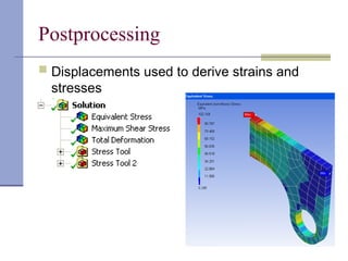
 Postprocessing
 Obtain other results (stresses, heat fluxes)

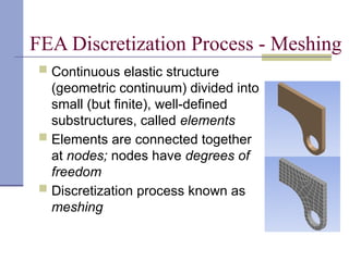
4. FEA Discretization Process - Meshing
 Continuous elastic structure
(geometric continuum) divided into
small (but finite), well-defined
substructures, called elements
 Elements are connected together
at nodes; nodes have degrees of
freedom
 Discretization process known as
meshing

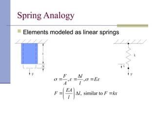
5. Spring Analogy
 Elements modeled as linear springs
, ,
, similar to
F l
E
A l
EA
F l F kx
l
   

  
 
  
 
 

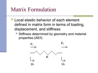
6. Matrix Formulation
 Local elastic behavior of each element
defined in matrix form in terms of loading,
displacement, and stiffness
 Stiffness determined by geometry and material
properties (AE/l)

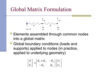
7. Global Matrix Formulation
 Elements assembled through common nodes
into a global matrix
 Global boundary conditions (loads and
supports) applied to nodes (in practice,
applied to underlying geometry)
1 1 2 2 1
2 2 2 2
F K K K U
F K K U
 
     

     

     

8. Solution
 Matrix operations used to determine unknown
dof’s (e.g., nodal displacements)
 Run time proportional to #nodes/elements
 Error messages
 “Bad” elements
 Insufficient disk space, RAM
 Insufficiently constrained

9. Postprocessing
 Displacements used to derive strains and
stresses

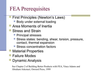
10. FEA Prerequisites
 First Principles (Newton’s Laws)
 Body under external loading
 Area Moments of Inertia
 Stress and Strain
 Principal stresses
 Stress states: bending, shear, torsion, pressure,
contact, thermal expansion
 Stress concentration factors
 Material Properties
 Failure Modes
 Dynamic Analysis
See Chapter 2 of Building Better Products with FEA, Vince Adams and
Abraham Askenazi, Onward Press, 1999

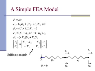
11. A Simple FEA Model





































2
1
2
2
2
2
1
2
1
2
2
1
2
2
2
2
1
2
1
1
2
1
2
2
2
1
2
1
1
1
)
(
)
(
)
(
0
)
(
0
)
(
U
U
K
K
K
K
K
F
F
U
K
U
K
F
U
K
U
K
K
F
K
U
U
F
K
U
U
K
U
F
Kx
F
Stiffness matrix

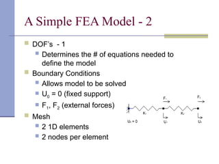
12. A Simple FEA Model - 2
 DOF’s - 1
 Determines the # of equations needed to
define the model
 Boundary Conditions
 Allows model to be solved
 U0 = 0 (fixed support)
 F1, F2 (external forces)
 Mesh
 2 1D elements
 2 nodes per element

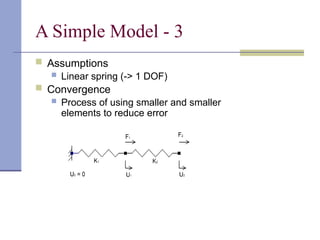
13. A Simple Model - 3
 Assumptions
 Linear spring (-> 1 DOF)
 Convergence
 Process of using smaller and smaller
elements to reduce error

14. Finite Element Analysis
Introduction