
Recommended
More Related Content
What's hot
What's hot (19)
Similar to Tham khao ofdm tutorial
Similar to Tham khao ofdm tutorial (20)
Recently uploaded
Recently uploaded (20)
Tham khao ofdm tutorial
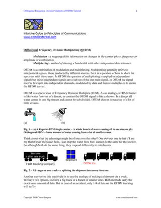
- 1. Orthogonal Frequency Division Multiplex (OFDM) Tutorial 1 Intuitive Guide to Principles of Communications www.complextoreal.com Orthogonal Frequency Division Multiplexing (OFDM) Modulation - a mapping of the information on changes in the carrier phase, frequency or amplitude or combination. Multiplexing - method of sharing a bandwidth with other independent data channels. OFDM is a combination of modulation and multiplexing. Multiplexing generally refers to independent signals, those produced by different sources. So it is a question of how to share the spectrum with these users. In OFDM the question of multiplexing is applied to independent signals but these independent signals are a sub-set of the one main signal. In OFDM the signal itself is first split into independent channels, modulated by data and then re-multiplexed to create the OFDM carrier. OFDM is a special case of Frequency Division Multiplex (FDM). As an analogy, a FDM channel is like water flow out of a faucet, in contrast the OFDM signal is like a shower. In a faucet all water comes in one big stream and cannot be sub-divided. OFDM shower is made up of a lot of little streams. (a) (b) Fig. 1 – (a) A Regular-FDM single carrier – A whole bunch of water coming all in one stream. (b) Orthogonal-FDM – Same amount of water coming from a lot of small streams. Think about what the advantage might be of one over the other? One obvious one is that if I put my thumb over the faucet hole, I can stop the water flow but I cannot do the same for the shower. So although both do the same thing, they respond differently to interference. Fig. 2 – All cargo on one truck vs. splitting the shipment into more than one. Another way to see this intuitively is to use the analogy of making a shipment via a truck. We have two options, one hire a big truck or a bunch of smaller ones. Both methods carry the exact same amount of data. But in case of an accident, only 1/4 of data on the OFDM trucking will suffer. Copyright 2004 Charan Langton www.complextoreal.com
- 2. Orthogonal Frequency Division Multiplex (OFDM) Tutorial 2 These four smaller trucks when seen as signals are called the sub-carriers in an OFDM system and they must be orthogonal for this idea to work. The independent sub-channels can be multiplexed by frequency division multiplexing (FDM), called multi-carrier transmission or it can be based on a code division multiplex (CDM), in this case it is called multi-code transmission. In this tutorial we will only talk about the multi-carrier FDM or OFDM. Fig. 3 – Multi-carrier FDM and Multi-code division multiplex The importance of being orthogonal The main concept in OFDM is orthogonality of the sub-carriers. Since the carriers are all sine/cosine wave, we know that area under one period of a sine or a cosine wave is zero. This is easily shown. Positive and negative area cancel. Positive and negative area cancel. +Area +Area +Area - - Fig. 4 - The area under a sine and a cosine wave over one period is always zero. Let's take a sine wave of frequency m and multiply it by a sinusoid (sine or a cosine) of a frequency n, where both m and n are integers. The integral or the area under this product is given by Copyright 2004 Charan Langton www.complextoreal.com
- 3. Orthogonal Frequency Division Multiplex (OFDM) Tutorial 3 ( ) sin sinf t mwt n= × wt (1) f t wt nwt( ) sin *sin= Sine wave multiplied by another of a different harmonic Figure 5 - The area under a sine wave multiplied by its own harmonic is always zero. By the simple trigonometric relationship, this is equal to a sum of two sinusoids of frequencies (n-m) and (n+m) 1 1 cos( ) cos( ) 2 2 m n m n= − − + These two components are each a sinusoid, so the integral is equal to zero over one period. 2 2 0 0 1 1 cos( ) cos( ) 2 2 0 0 m n t m n t π π ω ω= − − + = − ∫ ∫ We conclude that when we multiply a sinusoid of frequency n by a sinusoid of frequency m/n, the area under the product is zero. In general for all integers n and m, si are all orthogonal to each other. These frequencies are called harmonics. n ,cos ,cos ,sinmx mx nx nx This idea is key to understanding OFDM. The orthogonality allows simultaneous transmission on a lot of sub-carriers in a tight frequency space without interference from each other. In essence this is similar to CDMA, where codes are used to make data sequences independent (also orthogonal) which allows many independent users to transmit in same space successfully. OFDM is a special case of FDM (just as it says in its name, OFDM) Let’s first look at what a Frequency Division Multiplexing FDM is. If I have a bandwidth that goes from frequency a to b, I can subdivide this into a frequency space of four equal spaces. In frequency space the modulated carriers would look like this. Copyright 2004 Charan Langton www.complextoreal.com
- 4. Orthogonal Frequency Division Multiplex (OFDM) Tutorial 4 ba c1 c2 c3 c4 Fig. 6 – FDM carriers are placed to next to each other. The frequencies a and b can be anything, integer or non-integer since no relationship is implied between a and b. Same is true of the carrier center frequencies which are based on frequencies that do not have any special relationship to each other. But, what if frequency c1 and cn were such that for any n, an integer, the following holds. (2)1nc n c= × So that 2 1 3 1 4 1 2 3 4 c c c c c c = = = All three of these frequencies are harmonic to c1. In this case, since these carriers are orthogonal to each other, when added together, they do not interfere with each other. In FDM, since we do not generally have frequencies that follow the above relationship, we get interference from neighbor carriers. To provide adjacent channel interference protection, signals are moved further apart. The symbols rate that can be carried by a PSK carrier of bandwidth b, is given by 2s l pR B B= = where Bl is lowpass bandwidth and Bp, the passband bandwidth. This relationship assumes a perfect Nyquist filtering with rolloff = 0.0. Since this is unachievable, we use root raised cosine filtering which for a roll-off of α gives the following relationship. 1 p s B R α = + So if we need three carriers, each of data rate = 20 Mbps, then we might place our BPSK carriers as shown below. With Rs = 20 and B = 20 x 1.25 = 25 MHz. Each carrier may be placed (25 + 2.5) 27.5 MHz apart allowing for a 10% guard band. The frequencies would not be orthogonal but in FDM we don’t care about this. It’s the guard band that helps keep interference under control. An example of OFDM using 4 sub-carriers Copyright 2004 Charan Langton www.complextoreal.com
- 5. Orthogonal Frequency Division Multiplex (OFDM) Tutorial 5 In OFDM we have N carriers, N can be anywhere from 16 to 1024 in present technology and depends on the environment in which the system will be used. Let’s examine the following bit sequence we wish to transmit and show the development of the ODFM signal using 4 sub-carriers. The signal has a symbol rate of 1 and sampling frequency is 1 sample per symbol, so each transition is a bit. Fig. 7 – A bit stream that will be modulated using a 4 carrier OFDM. First few bits are 1, 1, -1, -1, 1, 1, 1, -1, 1, -1, -1, -1, -1, 1, -1, -1, -1, 1,… Let’s now write these bits in rows of fours, since this demonstration will use only four sub- carriers. We have effectively done a serial to parallel conversion. Table I – Serial to parallel conversion of data bits. c1 c2 c3 c4 1 1 -1 -1 1 1 1 -1 1 -1 -1 -1 -1 1 -1 -1 -1 1 1 -1 -1 -1 1 1 Each column represents the bits that will be carried by one sub-carrier. Let’s start with the first carrier, c1. What should be its frequency? From the Nyquist sampling Theorem, we know that smallest frequency that can convey information has to be twice the information rate. In this case, the information rate per carrier will be 1/4 or 1 symbol per second total for all 4 carriers. So the smallest frequency that can carry a bit rate of 1/4 is 1/2 Hz. But we picked 1 Hz for convenience. Had I picked 1/2 Hz as my starting frequency, then my harmonics would have been 1, 3/2 and 2 Hz. I could have chosen 7/8 Hz to start with and in which the harmonics would be 7/4, 7/2, 21/2 Hz. We pick BPSK as our modulation scheme for this example. (For QPSK, just imagine the same thing going on in the Q channel, and then double the bit rate while keeping the symbol rate the same.) Note that I can pick any other modulation method, QPSK, 8PSK 32-QAM or whatever. No limit here on what modulation to use. I can even use TCM which provides coding in addition to modulation. Carrier 1 - We need to transmit 1, 1, 1 -1, -1, -1 which I show below superimposed on the BPSK carrier of frequency 1 Hz. First three bits are 1 and last three -1. If I had shown the Q channel of this carrier (which would be a cosine) then this would be a QPSK modulation. Copyright 2004 Charan Langton www.complextoreal.com
- 6. Orthogonal Frequency Division Multiplex (OFDM) Tutorial 6 Fig. 8 – Sub-carrier 1 and the bits it is modulating (the first column of Table I) Carrier 2 - The next carrier is of frequency 2 Hz. It is the next orthogonal/harmonic to frequency of the first carrier of 1 Hz. Now take the bits in the second column, marked c2, 1, 1, -1, 1, 1, -1 and modulate this carrier with these bits as shown in Fig. Fig. 9 – Sub-carrier 2 and the bits that it is modulating (the 2nd column of Table I) Carrier 3 – Carrier 3 frequency is equal to 3 Hz and fourth carrier has a frequency of 4 Hz. The third carrier is modulated with -1, 1, 1, -1, -1, 1 and the fourth with -1, -1, -1, -1, -1, -1, 1 from Table I. Fig. 10 – Sub-carrier 3 and 4 and the bits that they modulating (the 3rd and 4th columns of Table I) Copyright 2004 Charan Langton www.complextoreal.com
- 7. Orthogonal Frequency Division Multiplex (OFDM) Tutorial 7 Now we have modulated all the bits using four independent carriers of orthogonal frequencies 1 to 4 Hz. What we have done is taken the bit stream, distributed the bits, one bit at a time to the four sub-carriers as shown in figure below. Time C1 C2 C3 C4 Fig. 11 – OFDM signal in time and frequency domain. Now add all four of these modulated carriers to create the OFDM signal, often produced by a block called the IFFT. Fig. 12 – Functional diagram of an OFDM signal creation. The outlined part is often called an IFFT block. Copyright 2004 Charan Langton www.complextoreal.com
- 8. Orthogonal Frequency Division Multiplex (OFDM) Tutorial 8 Fig. 13 – The generated OFDM signal. Note how much it varies compared to the underlying constant amplitude sub-carriers. In short-hand, we can write the process above as 1 ( ) ( )sin(2 ) N n n c t m t ntπ = = ∑ (4) Eq. 4 is basically an equation of an Inverse FFT. Using Inverse FFT to create the OFDM symbol The equation 4 is essentially an inverse FFT. The IFFT block in the OFDM chain confuses people. So let’s examine briefly what an FFT/IFFT does. Copyright 2004 Charan Langton www.complextoreal.com
- 9. Orthogonal Frequency Division Multiplex (OFDM) Tutorial 9 (a) Time domain view (b) Frequency domain view Fig. 14 - The two views of a signal Forward FFT takes a random signal, multiplies it successively by complex exponentials over the range of frequencies, sums each product and plots the results as a coefficient of that frequency. The coefficients are called a spectrum and represent “how much” of that frequency is present in the input signal. The results of the FFT in common understanding is a frequency domain signal. We can write FFT in sinusoids as ∑ ∑ − = − = ⎟ ⎠ ⎞ ⎜ ⎝ ⎛ +⎟ ⎠ ⎞ ⎜ ⎝ ⎛ = 1 0 1 0 2 cos)( 2 sin)()( N n N n N kn nxj N kn nxkx ππ (5) Here x(n) are the coeffcients of the sines and cosines of frequency 2 /k Nπ , where k is the index of the frequencies over the N frequencies, and n is the time index. x(k) is the value of the spectrum for the kth frequeny and x(n) is the value of the signal at time n. In Fig. 14 (b), the x(k =1) = 1.0 is one such value. The inverse FFT takes this spectrum and converts the whole thing back to time domain signal by again successively multiplying it by a range of sinusoids. The equation for IFFT is ∑ ∑ − = − = ⎟ ⎠ ⎞ ⎜ ⎝ ⎛ −⎟ ⎠ ⎞ ⎜ ⎝ ⎛ = 1 0 1 0 2 cos)( 2 sin)()( N n N n N kn kxj N kn kxnX ππ (6) The difference between Eq. 5 and 6 is the type of coefficients the sinusoids are taking, and the minus sign, and that’s all. The coefficients by convention are defined as time domain samples x(k) for the FFT and X(n) frequency bin values for the IFFT. The two processes are a linear pair. Using both in sequence will give the original result back. Copyright 2004 Charan Langton www.complextoreal.com
- 10. Orthogonal Frequency Division Multiplex (OFDM) Tutorial 10 (a) a time domain signal comes out as a spectrum out of a FFT and IFFT. They both do the same thing. (b) A frequency domain signal comes out as a time domain signal out of a IFFT. c) The pair return back the original input. (d) The pair return back the input no matter what it is. (e) the pair is commutable so they can be reversed and they will still return the original input. Fig 15 – FFT and IFFT are a matched linear pair. Copyright 2004 Charan Langton www.complextoreal.com
- 11. Orthogonal Frequency Division Multiplex (OFDM) Tutorial 11 Column 1 of Table I the signal bits, can be considered the amplitudes of a certain range of sinusoids. So we can use the IFFT to produce a time domain signal. You say, they are already in time domain, how can we process a time domain signal to produce an another time domain signal? The answer is that we pretend that the input bits are not time domain representations but are frequency amplitudes which if you are thinking clearly, will see that that is what they are. In this way, we can take these bits and by using the IFFT, we can create an output signal which is actually a time-domain OFDM signal. The IFFT is a mathematical concept and does not really care what goes in and what goes out. As long as what goes in is amplitudes of some sinusoids, the IFFT will crunch these numbers to produce a correct time domain result. Both FFT and IFFT will produce identical results on the same input. But most of us are not used to thinking of FFT/IFFT this way. We insist that only spectrums go inside the IFFT. Keeping with that mindset, each row of Table I can be considered a spectrum as plotted below. These rows aren’t actually spectrums, but that does not matter. Each row spectrum has only 4 frequencies which are 1, 2, 3 and 4 Hz . Each of these spectrums can be converted to produce a time-domain signal which is exactly what an IFFT does. Only in this case, the input is really a time domain signal disguising as a spectrum.. Spectrum 1 -1.5 -1 -0.5 0 0.5 1 1.5 1 2 3 4 Frequency Amplitude Spectrum 2 -1.5 -1 -0.5 0 0.5 1 1.5 1 2 3 4 Frequency Amplitude Spectrum 3 -1.5 -1 -0.5 0 0.5 1 1.5 1 2 3 4 Frequency Amplitude Spectrum 4 -1.5 -1 -0.5 0 0.5 1 1.5 1 2 3 4 Frequency Amplitude Fig. 16 – The incoming block of bits can be seen as a four bin spectrum, The IFFT converts this “spectrum” to a time domain OFDM signal for one symbol, which actually has four bits in it. IFFT quickly computes the time-domain signal instead of having to do it one carrier at time and then adding. Calling this functionality IFFT may be more satisfying because we are producing a time domain signal, but it is also very confusing. Because FFT and IFFT are linear processes and completely reversible, it should be called a FFT instead of a IFFT. The results are the same whether you do FFT or IFFT. In literature you will see it listed as IFFT everywhere. You can show you cleverness by recognizing that this block can also be a FFT as long as on the receive side, you do the reverse. Copyright 2004 Charan Langton www.complextoreal.com
- 12. Orthogonal Frequency Division Multiplex (OFDM) Tutorial 12 The functional block diagram of how the signal is modulated/demodulated is given below. Fig 17 – The OFDM link functions Defining fading If the path from the transmitter to the receiver either has reflections or obstructions, we can get fading effects. In this case, the signal reaches the receiver from many different routes, each a copy of the original. Each of these rays has a slightly different delay and slightly different gain. The time delays result in phase shifts which added to main signal component (assuming there is one.) causes the signal to be degraded. Tree0 0 Line of sight path gain Pathdelay α τ = = 1 1 Secondary path gain Secondary pathdelay α τ = = k k Secondary path gain Secondary pathdelay α τ = = Faded path Reflected multipath 1 0 0 0 ( ) ( ) ex p K c k k k k k k h t t Compl ath gain Normalized path delay relativeto LOS difference in pathtime α δ τ α τ τ τ − = = − = = ∆ = − ∑ Fig. 18 – Fading is big problem for signals. The signal is lost and demodulation must have a way of dealing with it. Fading is particular problem when the link path is changing, such as for a moving car or inside a building or in a populated urban area with tall building. If we draw the interferences as impulses, they look like this Copyright 2004 Charan Langton www.complextoreal.com
- 13. Orthogonal Frequency Division Multiplex (OFDM) Tutorial 13 0α 1α kα 1∆ k∆0∆ Fig. 19 – Reflected signals arrive at a delayed time period and interfere with the main line of sight signal, if there is one. In pure Raleigh fading, we have no main signal, all components are reflected. In fading, the reflected signals that are delayed add to the main signal and cause either gains in the signal strength or deep fades. And by deep fades, we mean that the signal is nearly wiped out. The signal level is so small that the receiver can not decide what was there. The maximum time delay that occurs is called the delay spread of the signal in that environment. This delay spread can be short so that it is less than symbol time or larger. Both cases, cause different types of degradations to the signal. The delay spread of a signal changes as the environment is changing as all cell phone users know. Fig. 19 shows the spectrum of the signal, the dark line shows the response we wish the channel to have. It is like a door through which the signal has to pass. The door is large enough that it allows the signal to go through without bending or distortion. A fading response of the channels is something like shown in Fig.20 b, we note that at some frequencies in the band, the channel does not allow any information to go through, so called deep fades frequencies. This form of channel frequency response is called frequency selective fading because it does not occur uniformly across the band. It occurs at selected frequencies. And who selects these frequencies. Environment. If the environment is changing such as for a moving car, then this response is also changing and the receiver must have some way of dealing with it. Rayleigh fading is a term used when there is no direct component and all signals reaching the receiver are reflected. This type of environment is called Rayleigh fading. In general when the delay spread is less than one symbol, we get what is called flat fading. When delay spread is much larger than one symbol that it is called frequency-selective fading. Copyright 2004 Charan Langton www.complextoreal.com
- 14. Orthogonal Frequency Division Multiplex (OFDM) Tutorial 14 Fig. 20 – (a) The signal we want to send and the channel frequency response are well matched. (b) A fading channel has frequencies that do not allow anything to pass. Data is lost sporadically. (c) With OFDM, where we have many little sub-carriers, only a small sub-set of the data is lost due to fading. An OFDM signal offers an advantage in a channel that has a frequency selective fading response. As we can see, when we lay an OFDM signal spectrum against the frequency-selective response of the channel, only two sub-carriers are affected, all the others are perfectly OK. Instead of the whole symbol being knocked out, we lose just a small subset of the (1/N) bits. With proper coding, this can be recovered. The BER performance of an OFDM signal in a fading channel is much better than the performance of QPSK/FDM which is a single carrier wideband signal. Although the underlying BER of a OFDM signal is exactly the same as the underlying modulation, that is if 8PSK is used to modulate the sub-carriers, then the BER of the OFDM signal is same as the BER of 8PSK signal in Gaussian channel. But in channels that are fading, the OFDM offers far better BER than a wide band signal of exactly the same modulation. The advantage here is coming from the diversity of the multi-carrier such that the fading applies only to a small subset. In FDM carriers, often the signal is shaped with a Root Raised Cosine shape to reduce its bandwidth, in OFDM since the spacing of the carriers is optimal, there is a natural bandwidth advantage and use of RRC does not buy us as much. Copyright 2004 Charan Langton www.complextoreal.com
- 15. Orthogonal Frequency Division Multiplex (OFDM) Tutorial 15 Delay spread and the use of cyclic prefix to mitigate it You are driving in rain, and the car in front splashes a bunch of water on you. What do you do? You move further back, you put a little distance between you and the front car, far enough so that the splash won’t reach you. If we equate the reach of splash to delay spread of a splashed signal then we have a better picture of the phenomena and how to avoid it. Delayed splash from front symbol Symbol 1 Symbol 2 Fig. 21 – Delay spread is like the undesired splash you might get from the car ahead of you. In fading, the front symbol similarly throws a splash backwards which we wish to avoid. Increase distance from car in front to avoid splash. The reach of splash is same as the delay spread of a signal. Fig. 22a shows the symbol and its splash. In composite, these splashes become noise and affect the beginning of the next symbol as shown in (b). Fig. 21 – The PSK symbol and its delayed version. (a) The delayed, attenuated signal and (b) composite interference. To mitigate this noise at the front of the symbol, we will move our symbol further away from the region of delay spread as shown below. A little bit of blank space has been added between symbols to catch the delay spread. Fig 22 – Move the symbol back so the arriving delayed signal peters out in the gray region. No interference to the next symbol! But we can not have blank spaces in signals. This is won’t work for the hardware which likes to crank out signals continuously. So it’s clear we need to have something there. Why don’t we just let the symbol run longer as a first choice? Copyright 2004 Charan Langton www.complextoreal.com
- 16. Orthogonal Frequency Division Multiplex (OFDM) Tutorial 16 Fig. 23 – If we just extend the symbol, then the front of the symbol which is important to us since it allows figuring out what the phase of this symbol is, is now corrupted by the “splash”. We extend the symbol into the empty space, so the actual symbol is more than one cycle. But now the start of the symbol is still in the danger zone, and this start is the most important thing about our symbol since the slicer needs it in order to make a decision about the bit. We do not want the start of the symbol to fall in this region, so lets just slide the symbol backwards, so that the start of the original symbol lands at the outside of this zone. And then fill this area with something. Fig. 24 – If we move the symbol back and just put in convenient filler in this area, then not only we have a continuous signal but one that can get corrupted and we don’t care since we will just cut it out anyway before demodulating. Slide the symbol to start at the edge of the delay spread time and then fill the guard space with a copy of what turns out to be tail end of the symbol. 1. We want the start of the symbol to be out of the delay spread zone so it is not corrupted and 2. We start the signal at the new boundary such that the actual symbol edge falls out side this zone. We will be extending the symbol so it is 1.25 times as long, to do this, copy the back of the symbol and glue it in the front. In reality, the symbol source is continuous, so all we are doing is adjusting the starting phase and making the symbol period longer. But nearly all books talk about it as a copy of the tail end. And the reason is that in digital signal processing, we do it this way. Copyright 2004 Charan Langton www.complextoreal.com
- 17. Orthogonal Frequency Division Multiplex (OFDM) Tutorial 17 Original symbol Portion added in the front Copy this part at front Symbol 1 Symbol 2 Copy this part at front Original symbolExtension Fig. 25 – Cyclic prefix is this superfluous bit of signal we add to the front of our precious cargo, the symbol. This procedure is called adding a cyclic prefix. Since OFDM, has a lot of carriers, we would do this to each and every carrier. But that’s only in theory. In reality since the OFDM signal is a linear combination, we can add cyclic prefix just once to the composite OFDM signal. The prefix is any where from 10% to 25% of the symbol time. Here is an OFDM signal with period equal to 32 samples. We want to add a 25% cyclic shift to this signal. 1. First we cut pieces that are 32 samples long. 2. Then we take the last .25 (32) = 8 samples, copy and append them to the front as shown. Fig. 26 – The whole process can be done only once to the OFDM signal, rather than doing it to each and every sub-carrier. We add the prefix after doing the IFFT just once to the composite signal. After the signal has arrived at the receiver, first remove this prefix, to get back the perfectly periodic signal so it can be FFT’d to get back the symbols on each carrier. However, the addition of cyclic prefix which mitigates the effects of link fading and inter symbol interference, increases the bandwidth. Copyright 2004 Charan Langton www.complextoreal.com
- 18. Orthogonal Frequency Division Multiplex (OFDM) Tutorial 18 Fig 27 – Addition of Cyclic prefix to the OFDM signal further improves its ability to deal with fading and interference. Properties of OFDM Spectrum and performance 0 Rs 2Rs 3Rs 4Rs 5Rs-4Rs -3Rs -2Rs -Rs 0 Rs 2Rs 3Rs 4Rs 5Rs-4Rs -3Rs -2Rs -Rs Fig. 28 – The spectrum of an OFDM signal (without addition of cyclic prefix) is much more bandwidth efficient than QPSK. Unshaped QPSK signal produces a spectrum such that its bandwidth is equal to (1+ α )Rs. In OFDM, the adjacent carriers can overlap in the manner shown here. The addition of two carriers, now allows transmitting 3Rs over a bandwidth of -2Rs to 2Rs or total of 4Ts. This gives a bandwidth efficiency of 4/3 Hz per symbol for 3 carriers and 6/5 for 5 carriers. As more and more carriers are added, the bandwidth approaches, 1N N + bits per Hz. So the larger the number of carriers, the better. Here is a spectrum of an OFDM signal. Note that the out of band signal is down by 50 dB without any pulse shaping. Copyright 2004 Charan Langton www.complextoreal.com
- 19. Orthogonal Frequency Division Multiplex (OFDM) Tutorial 19 Fig. 29 – the spectrum of an OFDM signal with 1024 sub-carriers Compare this to the spectrum of a QPSK signal, not how much lower the sidebands are for OFDM and how much less is the variance. Fig. 30 – the spectrum of a QPSK signal Bit Error Rate performance The BER of an OFDM is only exemplary in a fading environment. We would not use OFDM is a straight line of sight link such as a satellite link. OFDM signal due to its amplitude variation does not behave well in a non-linear channel such as created by high power amplifiers on board satellites. Using OFDM for a satellite would require a fairly large backoff, on the order of 3 dB, so there must be some other compelling reason for its use such as when the signal is to be used for a moving user. Peak to average power ratio (PAPR) If a signal is a sum of N signals each of max amplitude equal to 1 v, then it is conceivable that we could get a max amplitude of N that is all N signals add at a moment at their max points. The PAPR is defined as Copyright 2004 Charan Langton www.complextoreal.com
- 20. Orthogonal Frequency Division Multiplex (OFDM) Tutorial 20 2 ( ) avg x t R P = Fig. 31 – AN OFDM signal is very noise like. It looks just like a composite multi-FDM signal. For an OFDM signal that has 128 carriers, each with normalized power of 1 w, then the max PAPR can be as large as log (128) or 21 dB. This is at the instant when all 128 carriers combine at their maximum point, unlikely but possible. The RMS PAPR will be around half this number or 10-12 dB. This same PAPR is seen in CDMA signals as well. The large amplitude variation we see in Fig. 12 increases in-band noise and increases the BER when the signal has to go through amplifier non-linearities. Large back off is required in such cases. This makes use of OFDM just as problematic as Multi-carrier FDM in high power amplifier applications such as satellite links. What can be done about the large PAPR? Several ideas are used to mitigate it. 1. Clipping We can just clip the signal at a desired power level. This reduces the PAPR but introduces other distortions and ICI. 2. Selective Mapping Multiply the data signal by a set of codes, do the IFFT on each and then pick the one with the least PAPR. This is essentially doing the process many times using a CDMA like code. 3. Partial IFFT Divide the signal in clusters, do IFFT on each and then combine these. So that if we subdivide 128 carrier in to a group of four 32 carriers, each, the max PAPR of each will be 12 dB instead of 21 for the full. Combine these four sequences to create the transmit signal. These are some of the things that people are doing to keep the effect of the non-linearity manageable. Synchronization. The other problem is that tight synchronization is needed. Often pilot tones are served in the sub- carrier space. These are used to lock on phase and to equalize the channel. Coding The sub-carriers are typically coded with Convolutional coding prior to going through IFFT. The coded version of OFDM is called COFDM or Coded OFDM. Parameters of real OFDM Copyright 2004 Charan Langton www.complextoreal.com
- 21. Orthogonal Frequency Division Multiplex (OFDM) Tutorial 21 The OFDM use has increased greatly in the last 10 years. It is now proposed for radio broadcasting such as in Eureka 147 standard and Digital Radio Mondiale (DRM). OFDM is used for modem/ADSL application where it coexists with phone line. For ADSL use, the channel, the phone line, is filtered to provide a high SNR. OFDM here is called Discrete Multi Tone (DMT.) (Remember the special filters on you phone line if you have cable modem.) OFDM is also in use in your wireless internet modem and this usage is called 802.11a. Let’s take a look at some parameters of this application of OFDM. The summary of these are given below. Data rates 6 Mbps to 48 Mbps Modulation BPSK, QPSK, 16 QAM and 64 QAM Coding Convolutional concatenated with Reed Solomon FFT size 64 with 52 sub-carriers uses, 48 for data and 4 for pilots. Subcarrier frequency spacing 20 MHz divided by 64 carriers or .3125 MHz FFT period Also called symbol period, 3.2 µsec = 1/∆f Guard duration One quarter of symbol time, 0.8 µsec Symbol time 4 µsec http://www.csee.wvu.edu/wcrl/public/jianofdm.pdf http://www.drm.org/indexdeuz.htm __________________________________________ This tutorial by Charan Langton www.complextoreal.com Copyright 2004 All Rights reserved Copyright 2004 Charan Langton www.complextoreal.com
- 22. Orthogonal Frequency Division Multiplex (OFDM) Tutorial 22 Copyright 1998, 2002 Charan Langton I can be contacted at mntcastle@earthlink.net Other tutorials at www.complextoreal.com Copyright 2004 Charan Langton www.complextoreal.com