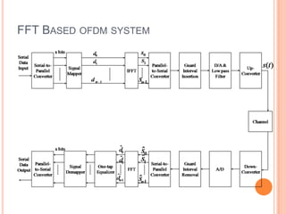
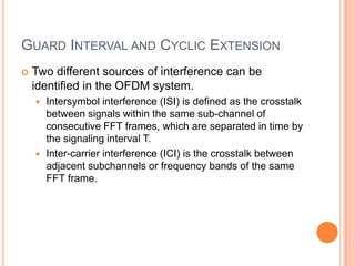
OFDM is a digital multi-carrier modulation technique that divides the available spectrum into several narrowband channels or subcarriers. It allows for high data rates by transmitting multiple digital signals over different subcarriers that are spaced closely together. The data is divided into several parallel data streams or channels, with each subcarrier modulated with a conventional modulation scheme like QAM at a low symbol rate. OFDM has become popular for applications like wireless networking due to its ability to combat multipath fading and its high spectral efficiency. It implements the orthogonal subcarriers using the inverse fast Fourier transform (IFFT) and fast Fourier transform (FFT) to generate the signal and decode it.

1. OFDM

2. INTRODUCTION
 Orthogonal frequency-division multiplexing (OFDM) is a frequency-
division multiplexing (FDM) scheme used as a digital multi-carrier
modulation method.
 A large number of closely-spaced orthogonal sub-carriers are used to carry
data.
 The data is divided into several parallel data streams or channels, one for
each sub-carrier.
 Each sub-carrier is modulated with a conventional modulation scheme
(such as QAM or PSK) at a low symbol rate, maintaining total data rates
similar to conventional single-carrier modulation schemes in the same
bandwidth.
 OFDM has developed into a popular scheme used in applications such as
digital video and audio broadcasting, wireless networking and WIMAX.

3. WHY OFDM?
 Can easily adapt to severe channel conditions without complex time-
domain equalization.
 Robust against narrow-band co-channel interference.
 Robust against inter-symbol interference (ISI) and fading caused by
multipath propagation.
 High spectral efficiency as compared to conventional modulation schemes,
spread spectrum, etc.
 Efficient implementation using Fast Fourier Transform (FFT).
 Low sensitivity to time synchronization errors.

4. FFT BASED OFDM SYSTEM

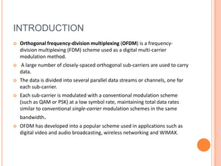
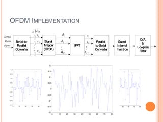
5. OFDM IMPLEMENTATION
x bits
x1 d1 s1
Serial
D/A
Data Serial-to- x2 Signal d2 s2 Parallel- Guard
&
Input Parallel Mapper IFFT to-Serial Interval
  Lowpass
Converter x n 1
(QPSK)
dn 1 sn 1
Converter Insertion
Filter
x= [1,0,1,1,0,0…] x1=[1,0] d1=[-1]
x2=[1,1] d2=[-i]
x3=[0,0] d3=[1]
…….. ……..

6. OFDM IMPLEMENTATION
x bits
x1 d1 s1
Serial
D/A
Data Serial-to- x2 Signal d2 s2 Parallel- Guard
&
Input Parallel Mapper IFFT to-Serial Interval
  Lowpass
Converter x n 1
(QPSK)
dn 1 sn 1
Converter Insertion
Filter
0.2
0.2 0.2
0.15
0.15 0.15
0.1
0.1 0.1
0.05 0.05 0.05
0 0
0
-0.05 -0.05
-0.05
-0.1 -0.1
-0.15 -0.1 -0.15
-0.2 -0.2
0 10 20 30 40 50 60
-0.15 70 0 10 20 30 40 50 60 70 80
-0.2
0 10 20 30 40 50 60 70 80

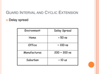
7. HOW?
 Discrete Fourier transform (DFT) and inverse DFT (IDFT) processes are
useful for implementing these orthogonal signals.
 Note that DFT and IDFT can be implemented efficiently by using fast
Fourier transform (FFT) and inverse fast Fourier transform (IFFT),
respectively.
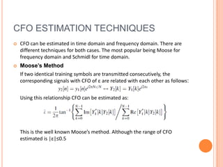
 In the OFDM transmission system, N-point IFFT is taken for the transmitted
symbols , so as to generate , the samples for the sum
of N orthogonal subcarrier signals.
 Let y[n] denote the received sample that corresponds to x[n] with the
additive noise w[n] (i.e., y[n] =x[n]+w[n]).
 Taking the N-point FFT of the received samples, , the noisy
version of transmitted symbols can be obtained in the receiver.

8. ORTHOGONALITY
 Two conditions must be considered for the
orthogonality between the subcarriers.
 Each subcarrier has exactly an integer number of cycles
in the FFT interval.
 The number of cycles between adjacent subcarriers
differs by exactly one.

9. ORTHOGONALITY
Time domain Frequency domain
Example of four subcarriers within one OFDM symbol Spectra of individual subcarriers

10. GUARD INTERVAL AND CYCLIC EXTENSION
 Two different sources of interference can be
identified in the OFDM system.
 Intersymbol interference (ISI) is defined as the crosstalk
between signals within the same sub-channel of
consecutive FFT frames, which are separated in time by
the signaling interval T.
 Inter-carrier interference (ICI) is the crosstalk between
adjacent subchannels or frequency bands of the same
FFT frame.

11. GUARD INTERVAL AND CYCLIC EXTENSION
 Delay spread
Environment Delay Spread
Home < 50 ns
Office ~ 100 ns
Manufactures 200 ~ 300 ns
Suburban < 10 us

12. GUARD INTERVAL AND CYCLIC EXTENSION
 For the purpose to eliminate the effect of ISI, the guard
interval could consist of no signals at all.
 Guard interval (or cyclic extension) is used in OFDM
systems to combat against multipath fading.
Tg :guard interval
Tdelay-spread : multi path delay spread
Tg > Tdelay-spread
 In that case, however, the problem of inter-carrier
interference (ICI) would arise.
 The reason is that there is no integer number of cycles
difference between subcarriers within the FFT interval.

13. GUARD INTERVAL AND CYCLIC EXTENSION
If T g < T dely-spread
Tg Symbol 1 Tg Symbol 2 Tg Symbol 3 Tg Symbol 4 ﹒ ﹒ ﹒ ﹒
Tg Symbol 1 Tg Symbol 2 Tg Symbol 3 ﹒ ﹒ ﹒ ﹒
Tdely-spread
If T g > T dely-spread
Tg Symbol 1 Tg Symbol 2 Tg Symbol 3 Tg Symbol 4 ﹒ ﹒ ﹒ ﹒
Tg Symbol 1 Tg Symbol 2 Tg Symbol 3 ﹒ ﹒ ﹒ ﹒
Tdely-spread

14. GUARD INTERVAL AND CYCLIC EXTENSION
 To eliminate ICI, the OFDM symbol is cyclically
extended in the guard interval.
 This ensures that delayed replicas of the OFDM
symbol always have an integer number of cycles
within the FFT interval, as long as the delay is
smaller than the guard interval.
Guard Interval
(Cyclic Extension)

15. GUARD INTERVAL AND CYCLIC EXTENSION
 Effect of multipath with zero signals in the guard
interval, the delayed subcarrier 2 causes ICI on
subcarrier 1 and vice versa.
Part of subcarrier #2
causing ICI on
subcarrier #1
Subcarrier #1
Delayed subcarrier #2
Guard time FFT integration time=1/carrier spacing Guard time FFT integration time=1/carrier spacing
OFDM symbol time OFDM symbol time

16. GUARD INTERVAL AND CYCLIC EXTENSION

17. CFO
 The carrier frequency offset (CFO) is caused by Doppler frequency shift fd .
 We intend to generate exactly the same carrier frequencies in the
transmitter and receiver, but ,there may be an unavoidable difference
between them due to the physically inherent nature of the oscillators. Let
fc and f ’c denote the carrier frequencies in the transmitter and receiver,
respectively. Let foffset denote their difference (i.e., foffset = fc - f ’c).
 Doppler frequency fd is determined by the carrier frequency fc and the
velocity v of the terminal (receiver) as
fd = (v.fc)/c
where c is the speed of light. Let us define the normalized CFO, Ɛ, as a
ratio of the CFO to subcarrier spacing Δf , shown as
Ɛ=(Foffset / Δf)
Let Ɛi and Ɛf denote the integer part and fractional part of Ɛ, respectively,
and therefore,
Ɛ=Ɛi+Ɛf, where Ɛi= |Ɛ|.

18. EFFECT OF INTEGER CARRIER FREQUENCY
OFFSET(IFO)
 Due to the IFO, the transmit signal X(k) is cyclic shifted by Ɛi in the receiver,
and thus producing X(k-Ɛi) in the kth subcarrier. Unless the cyclic shift is
compensated, it will incur a significant degradation in the BER
performance. However, we note that the orthogonality among the
subcarrier frequency components is not destroyed and thus, ICI does not
occur.

19. EFFECT OF FRACTIONAL CARRIER FREQUENCY
OFFSET(FFO)
 It is clear from this figure that amplitude and phase distortion becomes
severe as FFO increases.

21. CFO ESTIMATION TECHNIQUES
 CFO can be estimated in time domain and frequency domain. There are
different techniques for both cases. The most popular being Moose for
frequency domain and Schmidl for time domain.
 Moose’s Method
If two identical training symbols are transmitted consecutively, the
corresponding signals with CFO of ε are related with each other as follows:
Using this relationship CFO can be estimated as:
This is the well known Moose’s method. Although the range of CFO
estimated is |ε|≤0.5

22.  Schmidl’s and the Improvement method is different in terms of the
Pilot arrangement.
 In Schmidl method we use two repeated N/2 length long pilot
sequences.
 While in the Improvement method we use four repeated N/4 length
long pilot sequences.

23.  Schmidl Method
Here CFO estimation is done with a single step. We use the correlation
between the two PN sequences to determine an intermediate variable.
In is the sum of all noise, which can be regarded as AWGN when N is larger
enough.
CFO estimated by taking the phase of ϕ.

24.  Improvement Method
This estimation is done in two steps.
First we do a coarse estimation to get the coarse CFO value.
Then after correcting for this rough value we do a fine estimation on
the corrected signal to get a better approximation to the true value.
 Coarse Estimation
This estimation is done by the following iteration to get the
intermediate value.
Essentially we are correlating the first and fourth N/4 length pilot
symbols.
Coarse estimate is obtained by taking the phase of φ1.

25.  Correction
The received signal is corrected by accounting for the CFO
estimated.
 Fine Estimation
This estimation is done by the following iteration to get a second
intermediate value.
Here we are correlating the second and third N/4 length pilot
symbols. Where ε2=ε-ε1 the residual CFO.
Fine estimate is obtained by taking the phase of φ2.
The total CFO is the sum of the fine and coarse estimates.

26. COMPARISON BETWEEN SCHMIDL AND MOOSE

27. COMPARISON BETWEEN SCHMIDL AND IMPROVEMENT IN AWGN CHANNEL

28. COMPARISON BETWEEN SCHMIDL AND IMPROVEMENT IN COST 207
CHANNEL MODEL