Download to read offline
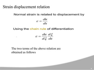
![Thus the normal strain relation can be written as
which can be written in matrix form as
where [B] is a row matrix called the strain-displacement matrix, given
by since x2 – x1 = element length = le
10](https://image.slidesharecdn.com/sushma-fem-201029163013/85/Expressions-for-shape-functions-of-linear-element-10-320.jpg)
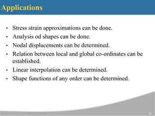
![Properties od stiffness matrix
The dimension of the global stiffness matrix is (nxn),
where n is total number d.o.f. of the body(or structure).
It is symmetric matrix.
It is singular matrix, and hence [K]-1 does not exist.
For global stiffness matrix, sum of any row or column
is equal to zero.
It is positive definite i.e. all diagonal elements are
nonzero and positive.
I tis banded matrix. That is, all elements outside the
band are zero.
11](https://image.slidesharecdn.com/sushma-fem-201029163013/85/Expressions-for-shape-functions-of-linear-element-11-320.jpg)


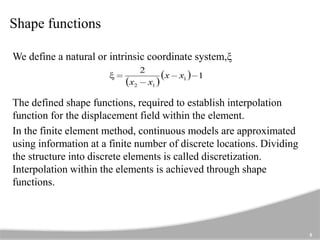
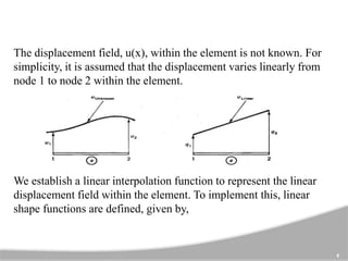
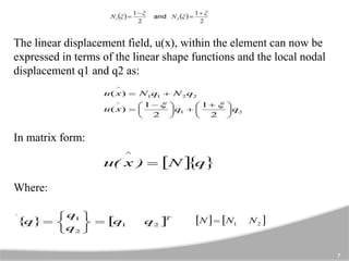
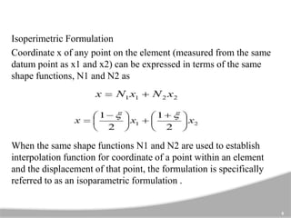
The document explains the use of linear shape functions in finite element modeling to interpolate solutions between discrete values at mesh nodes. It outlines the concepts of natural coordinates, the strain-displacement matrix, and properties of the stiffness matrix, emphasizing the importance of linear interpolation to estimate displacement fields within elements. Applications include stress-strain approximations, nodal displacement determination, and establishing relations between local and global coordinates.