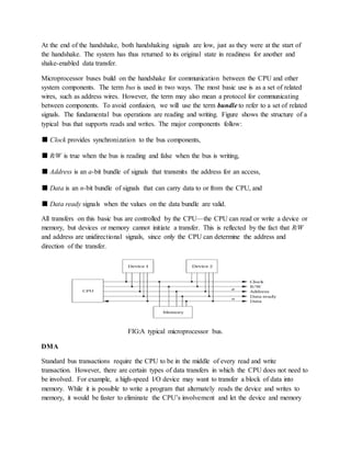
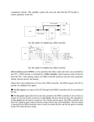
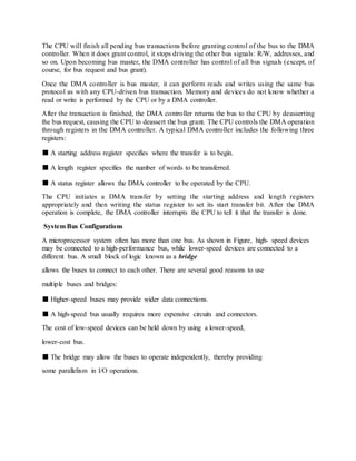
This document discusses bus-based computer systems and how they interconnect microprocessors, memory, and I/O devices using a CPU bus. It describes the basic components and functions of a CPU bus including address and data lines. It also discusses bus protocols using a four-cycle handshake and how direct memory access (DMA) allows bus transactions without CPU involvement by letting other devices become bus masters. The document concludes by discussing multiple bus systems and advanced bus architectures like AMBA.

1. Bus-Based Computer Systems
INTRODUCTION
In this chapter, we concentrate on bus-based computer systems created using microprocessors,
I/O devices, and memory components. The microprocessor is an important element of the
embedded computing system, but it cannot do its job without memories and I/O devices. We
need to understand how to interconnect microprocessors and devices using the CPU bus.
THE CPU BUS
A computer system encompasses much more than the CPU;it also includes memory and I/O
devices. The bus is the mechanism by which the CPU communicates with memory and devices.
A bus is, at a minimum, a collection of wires, but the bus also defines a protocol by which the
CPU, memory, and devices communicate. One of the major roles of the bus is to provide an
interface to memory. (Of course, I/O devices also connect to the bus.) Based on understanding of
the bus, we study the characteristics of memory components in this section.
Bus Protocols
The basic building block of most bus protocols is the four-cycle handshake. The handshake
ensures that when two devices want to communicate, one is ready to transmit and the other is
ready to receive. The handshake uses a pair of wires dedicated to the handshake: enq (meaning
enquiry) and ack (meaning acknowledge). Extra wires are used for the data transmitted during
the handshake. The four cycles are described below.
1. Device 1 raises its output to signal an enquiry, which tells device 2 that it should get ready
to listen for data.
2. When device 2 is ready to receive, it raises its output to signal an acknowledgment. At this
point, devices 1 and 2 can transmit or receive.
3. Once the data transfer is complete, device 2 lowers its output, signaling that it has received the
data.
4. After seeing that ack has been released, device 1 lowers its output.

2. At the end of the handshake, both handshaking signals are low, just as they were at the start of
the handshake. The system has thus returned to its original state in readiness for another and
shake-enabled data transfer.
Microprocessor buses build on the handshake for communication between the CPU and other
system components. The term bus is used in two ways. The most basic use is as a set of related
wires, such as address wires. However, the term may also mean a protocol for communicating
between components. To avoid confusion, we will use the term bundle to refer to a set of related
signals. The fundamental bus operations are reading and writing. Figure shows the structure of a
typical bus that supports reads and writes. The major components follow:
■ Clock provides synchronization to the bus components,
■ R/W is true when the bus is reading and false when the bus is writing,
■ Address is an a-bit bundle of signals that transmits the address for an access,
■ Data is an n-bit bundle of signals that can carry data to or from the CPU, and
■ Data ready signals when the values on the data bundle are valid.
All transfers on this basic bus are controlled by the CPU—the CPU can read or write a device or
memory, but devices or memory cannot initiate a transfer. This is reflected by the fact that R/W
and address are unidirectional signals, since only the CPU can determine the address and
direction of the transfer.
FIG:A typical microprocessor bus.
DMA
Standard bus transactions require the CPU to be in the middle of every read and write
transaction. However, there are certain types of data transfers in which the CPU does not need to
be involved. For example, a high-speed I/O device may want to transfer a block of data into
memory. While it is possible to write a program that alternately reads the device and writes to
memory, it would be faster to eliminate the CPU’s involvement and let the device and memory

3. communicate directly. This capability requires that some unit other than the CPU be able to
control operations on the bus.
Fig: Bus signals for multiplexing address and data.
Fig: Bus signals for multiplexing address and data.
Direct memory access (DMA) is a bus operation that allows reads and writes not controlled by
the CPU. A DMA transfer is controlled by a DMA controller, which requests control of the bus
from the CPU. After gaining control, the DMA controller performs read and write operations
directly between devices and memory.
Figure shows the configuration of a bus with a DMA controller. The DMA requires the CPU to
provide two additional bus signals:
■ The bus request is an input to the CPU through which DMA controllers ask for ownership of
the bus.
■ The bus grant signals that the bus has been granted to the DMA controller.A device that can
initiate its own bus transfer is known as a bus master. Devices that do not have the capability to
be bus masters do not need to connect to a bus request and bus grant. The DMA controller uses
these two signals to gain control of the bus using a classic four-cycle handshake. The bus request
is asserted by the DMA controller when it wants to control the bus, and the bus grant is asserted
by the CPU when the bus is ready.

4. The CPU will finish all pending bus transactions before granting control of the bus to the DMA
controller. When it does grant control, it stops driving the other bus signals: R/W, addresses, and
so on. Upon becoming bus master, the DMA controller has control of all bus signals (except, of
course, for bus request and bus grant).
Once the DMA controller is bus master, it can perform reads and writes using the same bus
protocol as with any CPU-driven bus transaction. Memory and devices do not know whether a
read or write is performed by the CPU or by a DMA controller.
After the transaction is finished, the DMA controller returns the bus to the CPU by deasserting
the bus request, causing the CPU to deassert the bus grant. The CPU controls the DMA operation
through registers in the DMA controller. A typical DMA controller includes the following three
registers:
■ A starting address register specifies where the transfer is to begin.
■ A length register specifies the number of words to be transferred.
■ A status register allows the DMA controller to be operated by the CPU.
The CPU initiates a DMA transfer by setting the starting address and length registers
appropriately and then writing the status register to set its start transfer bit. After the DMA
operation is complete, the DMA controller interrupts the CPU to tell it that the transfer is done.
System Bus Configurations
A microprocessor system often has more than one bus. As shown in Figure, high- speed devices
may be connected to a high-performance bus, while lower-speed devices are connected to a
different bus. A small block of logic known as a bridge
allows the buses to connect to each other. There are several good reasons to use
multiple buses and bridges:
■ Higher-speed buses may provide wider data connections.
■ A high-speed bus usually requires more expensive circuits and connectors.
The cost of low-speed devices can be held down by using a lower-speed,
lower-cost bus.
■ The bridge may allow the buses to operate independently, thereby providing
some parallelism in I/O operations.

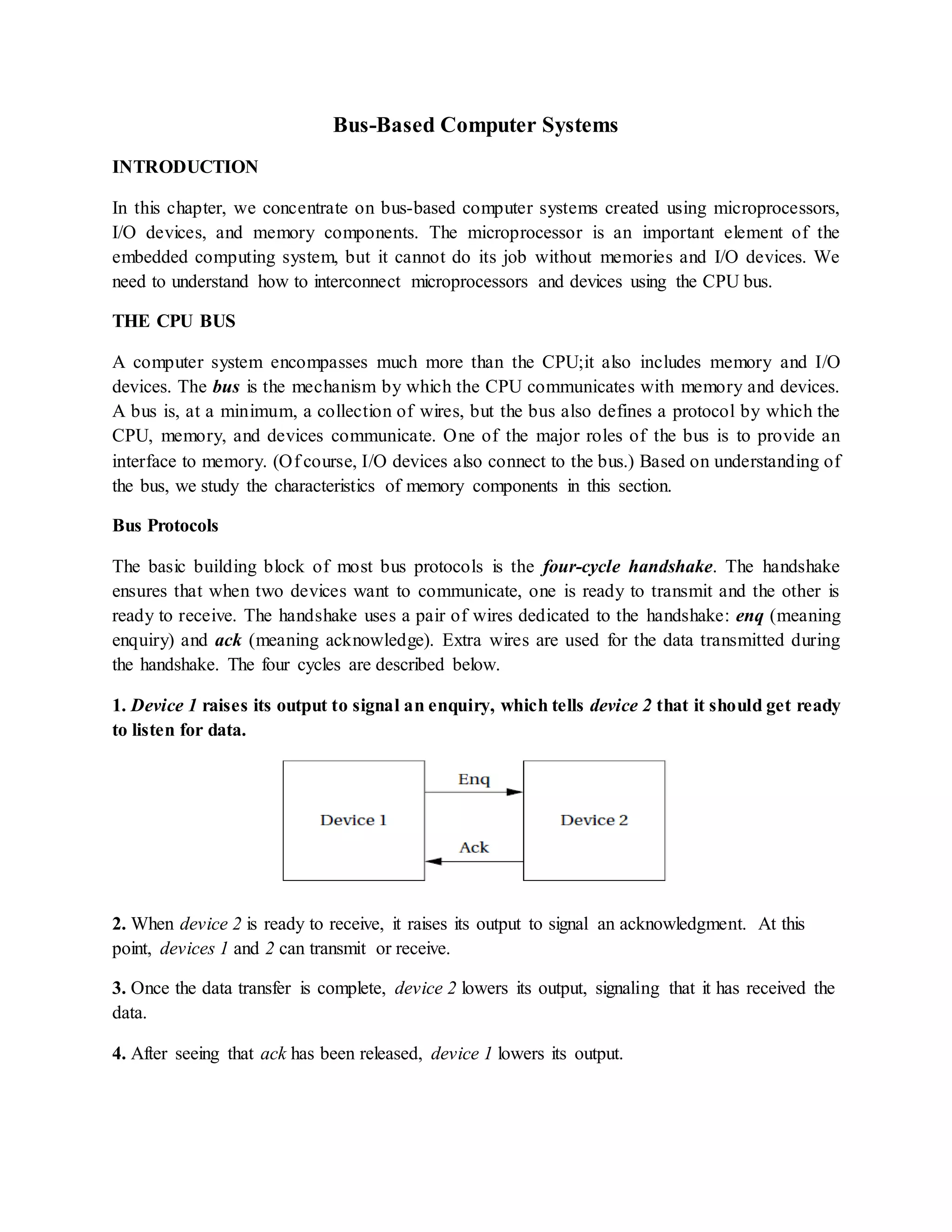
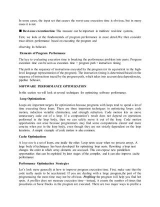
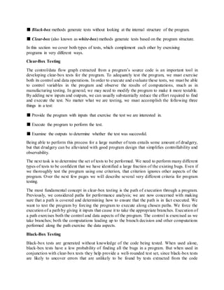
5. FIGURE A multiple bus system.
AMBA Bus
Since the ARM CPU is manufactured by many different vendors, the bus provided off-chip can
vary from chip to chip. ARM has created a separate bus specification for single-chip systems.
The AMBA bus [ARM99A] supports CPUs, memories, and peripherals integrated in a system-
on-silicon. As shown in Figure 4.14, the AMBA specification includes two buses. The AMBA
high-performance bus (AHB) is optimized for high-speed transfers and is directly connected to
the CPU. It supports several high-performance features: pipelining, burst transfers, split
transactions,
and multiple bus masters. A bridge can be used to connect the AHB to an AMBA peripherals bus
(APB). This bus is designed to be simple and easy to implement; it also consumes relatively
little power. The AHB assumes that all peripherals act as slaves, simplifying the logic required
in both the peripherals and the bus controller. It also does not perform pipelined operations,
which simplifies the bus logic.
PROGRAM-LEVEL PERFORMANCE ANALYSIS
Because embedded systems must perform functions in real time, we often need to know how fast
a program runs. The techniques we use to analyze program execution time are also helpful in

6. analyzing properties such as power consumption. In this section, we study how to analyze
programs to estimate their run times. We also examine how to optimize programs to improve
their execution times; of course, optimization relies on analysis. In order to understand the total
execution time of our program, we must look at execution paths, which in general are far longer
than the pipeline and cache window The pipeline and cache influence execution time,but
execution time is a global property of the program.While we might hope that the execution time
of programs could be precisely determined, this is in fact difficult to do in practice:
■ The execution time of a program often varies with the input data values because those values
select different execution paths in the program. For example, loops may be executed a varying
number of times, and different branches may execute blocks of varying complexity.
■ The cache has a major effect on program performance, and once again, the cache’s behavior
depends in part on the data values input to the program.
■ Execution times may vary even at the instruction level. Floating-point operations are the most
sensitive to data values, but the normal integer execution pipeline can also introduce data-
dependent variations. In general, the execution
time of an instruction in a pipeline depends not only on that instruction but on the instructions
around it in the pipeline.
We can measure program performance in several ways:
■ Some microprocessor manufacturers supply simulators for their CPUs: The simulator runs on
a workstation or PC, takes as input an executable for the microprocessor along with input
data,and simulates the execution of that program. Some of these simulato rs go beyond
functional simulation to measure the execution time of the program. Simulation is clearly slower
than executing the program on the actual microprocessor, but it also provides much greater
visibility during execution. Be careful—some microprocessor performance simulators are not
100% accurate, and simulation of I/O-intensive code may be difficult.
■ A timer connected to the microprocessor bus can be used to measure performance of
executing sections of code. The code to be measured would reset and start the timer at its start
and stop the timer at the end of execution. The length of the program that can be measured is
limited by the accuracy of the timer.
■ A logic analyzer can be connected to the microprocessor bus to measure the start and stop
times of a code segment. This technique relies on the code being able to produce identifiable
events on the bus to identify the start and stop of execution. The length of code that can be
measured is limited by the size of the logic analyzer’s buffer.
We are interested in the following three different types of performance measures on programs:
■ Average-case execution time This is the typical execution time we would expect for typical
data. Clearly, the first challenge is defining typical inputs.
■ Worst-case execution time The longest time that the program can spend on any input
sequence is clearly important for systems that must meet deadlines.

7. In some cases, the input set that causes the worst-case execution time is obvious, but in many
cases it is not.
■ Best-case execution time This measure can be important in multirate real-time systems,
First, we look at the fundamentals of program performance in more detail.We then consider
trace-driven performance based on executing the program and
observing its behavior.
Elements of Program Performance
The key to evaluating execution time is breaking the performance problem into parts. Program
execution time can be seen as execution time = program path + instruction timing
The path is the sequence of instructions executed by the program (or its equivalent in the high-
level language representation of the program). The instruction timing is determined based on the
sequence of instructions traced by the program path, which takes into account data dependencies,
pipeline behavior,
SOFTWARE PERFORMANCE OPTIMIZATION
In this section we will look at several techniques for optimizing software performance.
Loop Optimizations
Loops are important targets for optimization because programs with loops tend to spend a lot of
time executing those loops. There are three important techniques in optimizing loops: code
motion, induction variable elimination, and strength reduction. Code motion lets us move
unnecessary code out of a loop. If a computation’s result does not depend on operations
performed in the loop body, then we can safely move it out of the loop. Code motion
opportunities can arise because programmers may find some computations clearer and more
concise when put in the loop body, even though they are not strictly dependent on the loop
iterations. A simple example of code motion is also common.
Cache Optimizations
A loop nest is a set of loops, one inside the other. Loop nests occur when we process arrays. A
large body of techniques has been developed for optimizing loop nests. Rewriting a loop nest
changes the order in which array elements are accessed. This can expose new parallelism
opportunities that can be exploited by later stages of the compiler, and it can also improve cache
performance
Performance Optimization Strategies
Let’s look more generally at how to improve program execution time. First, make sure that the
code really needs to be accelerated. If you are dealing with a large program,the part of the
programusing the most time may not be obvious. Profiling the program will help you find hot
spots. A profiler does not measure execution time—instead, it counts the number of times that
procedures or basic blocks in the program are executed. There are two major ways to profile a

8. program:We can modify the executable program by adding instructions that increment a location
every time the program passes that point in the program; or we can sample the program counter
during execution and keep track of the distribution of PC values.
Profiling adds relatively little overhead to the program and it gives us some useful information
about where the program spends most of its time. You may be able to redesign your algorithm to
improve efficiency. Examining asymptotic performance is often a good guide to efficiency.
Doing fewer operations is usually the key to performance. In a few cases, however, brute force
may provide a better implementation. A seemingly simple high-level language statement may in
fact hide a very long sequence of operations that slows down the algorithm. Using dynamically
allocated memory is one example, since managing the heap takes time but is hidden from the
programmer. For example, a sophisticated algorithm that uses dynamic storage may be slower in
practice than an algorithm that performs more operations on statically allocated memory.
Finally, you can look at the implementation of the program itself. A few hints on program
implementation are summarized below.
■ Try to use registers efficiently. Group accesses to a value together so that the value can be
brought into a register and kept there.
■ Make use of page mode accesses in the memory system whenever possible. Page mode reads
and writes eliminate one step in the memory access. You can increase use of page mode by
rearranging your variables so that more can be referenced contiguously.
■ Analyze cache behavior to find major cache conflicts. Restructure the code to eliminate as
many of these as you can as follows:
—For instruction conflicts, if the offending code segment is small, try to rewrite the segment to
make it as small as possible so that it better fits into the cache. Writing in assembly language
may be necessary. For conflicts across larger spans of code, try moving the instructions or
padding with NOPs.
—For scalar data conflicts, move the data values to different locations to reduce conflicts.
—For array data conflicts, consider either moving the arrays or changing your array access
patterns to reduce conflicts.
PROGRAM-LEVEL ENERGY AND POWER ANALYSIS AND OPTIMIZATION
Power consumption is a particularly important design metric for battery-powered systems
because the battery has a very limited lifetime. However, power consumption is increasingly
important in systems that run off the power grid. Fast chips run hot, and controlling power
consumption is an important element of increasing reliability and reducing system cost.
Ultimately, we must consume the energy required to perform necessary computations. However,
there are opportunities for saving power. Examples appear below.
■ We may be able to replace the algorithms with others that do things in clever ways that
consume less power.

9. ■ Memory accesses are a major component of power consumption in many applications. By
optimizing memory accesses we may be able to significantly reduce power.
■ We may be able to turn off parts of the system—such as subsystems of the CPU, chips in the
system, and so on—when we do not need them in order to save power.
The first step in optimizing a program’s energy consumption is knowing how much energy the
program consumes. It is possible to measure power consumption for an instruction or a small
code fragment. The technique, illustrated in Figure, executes the code under test over and over in
a loop. By measuring the current flowing into the CPU, we are measuring the power
consumption of the complete loop, including both the body and other code. By separately
measuring the power consumption of a loop with no body (making sure, of course, that the
compiler hasn’t optimized away the empty loop),we can calculate the power consumption of the
loop body code as the difference between the full loop and the bare loop energy cost of an
instruction.
Several factors contribute to the energy consumption of the program.
■ Energy consumption varies somewhat from instruction to instruction.
■ The sequence of instructions has some influence.
■ The opcode and the locations of the operands also matter.
Choosing which instructions to use can make some difference in a program’s energy
consumption, but concentrating on the instruction opcodes has limited payoffs in most CPUs.
The program has to do a certain amount of computation to perform its function. While there may
be some clever ways to perform that computation, the energy cost of the basic computation will
change only a fairly small amount compared to the total system energy consumption, and usually
only after a great deal of effort. We are further hampered in our ability to optimize instruction
level energy consumption because most manufacturers do not provide detailed, instruction-level
energy consumption figures for their processors.
In many applications, the biggest payoff in energy reduction for a given amount of designer
effort comes from concentrating on the memory system. As a result, the biggest payoffs in
energy optimization come from properly organizing instructions and data in memory. Accesses
to registers are the most energy efficient; cache accesses are more energy efficient than main
memory accesses. Caches are an important factor in energy consumption.
As the instruction cache size increases, the energy cost of the software on the CPU declines, but
the instruction cache comes to dominate the energy consumption. Experiments like this on
several benchmarks show that many programs have sweet spots in energy consumption. If the
cache is too small, the program runs slowly and the system consumes a lot of power due to the
high cost of main memory accesses. If the cache is too large, the power consumption is high
without a corresponding payoff in performance. At intermediate values, the execution time and
power consumption are both good.
The best overall advice is that high performance = low power. Generally speaking, making the
program run faster also reduces energy consumption. Clearly, the biggest factor that can be

10. reasonably well controlled by the programmer is the memory access patterns. If the program can
be modified to reduce instruction or data cache conflicts, for example, the energy required by the
memory system can be significantly reduced. The effectiveness of changes such as reordering
instructions or selecting different instructions depends on the processor involved, but they are
generally less effective than cache optimizations.
A few optimizations mentioned previously for performance are also often useful for improving
energy consumption:
■ Try to use registers efficiently. Group accesses to a value together so that the value can be
brought into a register and kept there.
■ Analyze cache behavior to find major cache conflicts. Restructure the code to eliminate as
many of these as you can:
—For instruction conflicts, if the offending code segment is small, try to rewrite the segment to
make it as small as possible so that it better fits into the cache. Writing in assembly language
may be necessary. For conflicts across larger spans of code, try moving the instructions or
padding with NOPs.
—For scalar data conflicts, move the data values to different locations to reduce conflicts.
—For array data conflicts, consider either moving the arrays or changing your array access
patterns to reduce conflicts.
■ Make use of page mode accesses in the memory system whenever possible. Page mode reads
and writes eliminate one step in the memory access, saving a considerable amount of power.
ANALYSIS AND OPTIMIZATION OF PROGRAM SIZE
The memory footprint of a program is determined by the size of its data and instructions. Both
must be considered to minimize program size. Data provide an excellent opportunity for
minimizing size because the data are most highly dependent on programming style. Because
inefficient programs often keep several copies of data, identifying and eliminating duplications
can lead to significant memory savings usually with little performance penalty. Buffers should be
sized carefully—rather than defining a data array to a large size that the program will never
attain, determine the actual maximum amount of data held in the buffer and allocate the array
accordingly. Data can sometimes be packed, such as by storing several flags in a single word and
extracting them by using bit-level operations. A very low-level technique for minimizing data is
to reuse values. For instance, if several constants happen to have the same value, they can be
mapped to the same location. Data buffers can often be reused at several different points in the
program.
This technique must be used with extreme caution, however, since subsequent versions of the
program may not use the same values for the constants. A more generally applicable technique is
to generate data on the fly rather than store it. Of course, the code required to generate the data
takes up space in the program, but when complex data structures are involved there may be some
net space savings from using code to generate data.

11. Minimizing the size of the instruction text of a program requires a mix of high-level program
transformations and careful instruction selection. Encapsulating functions in subroutines can
reduce program size when done carefully. Because subroutines have overhead for parameter
passing that is not obvious from the high-level language code, there is a minimum-size function
body for which a subroutine makes sense. Architectures that have variable-size instruction
lengths are particularly good candidates for careful coding to minimize program size, which
may require assembly language coding of key program segments. There may also be cases in
which one or a sequence of instructions is much smaller than alternative implementations for
example, a multiply-accumulate instruction may be both smaller and faster than separate
arithmetic operations. When reducing the number of instructions in a program, one important
technique is the proper use of subroutines. If the program performs identical operations
repeatedly, these operations are natural candidates for subroutines. Even if the operations vary
somewhat, you may be able to construct a properly parameterized subroutine that saves space. Of
course, when considering the code size savings, the subroutine linkage code must be counted into
the equation. There is extra code not only in the subroutine body but also in each call to the
subroutine that handles parameters. In some cases, proper instruction selection may reduce code
size; this is particularly true in CPUs that use variable-length instructions.
Some microprocessor architectures support dense instruction sets, specially designed instruction
sets that use shorter instruction formats to encode the instructions. The ARM Thumb instruction
set and the MIPS-16 instruction set for the MIPS architecture are two examples of this type of
instruction set. In many cases, a microprocessor that supports the dense instruction set also
supports the normal instruction set, although it is possible to build a microprocessor that executes
only the dense instruction set. Special compilation modes produce the program in terms of the
dense instruction set. Program size of course varies with the type of program,but programs using
the dense instruction set are often 70 to 80% of the size of the standard instruction set
equivalents.
PROGRAM VALIDATION AND TESTING
Complex systems need testing to ensure that they work as they are intended. But bugs can be
subtle, particularly in embedded systems, where specialized hardware and real-time
responsiveness make programming more challenging. Fortunately, there are many available
techniques for software testing that can help us generate a comprehensive set of tests to ensure
that our system works properly. We examine the role of validation in the overall design
methodology. In this section, we concentrate on nuts-and-bolts techniques for creating a good set
of tests for a given program.
The first question we must ask ourselves is how much testing is enough. Clearly, we cannot test
the program for every possible combination of inputs. Because we cannot implement an infinite
number of tests, we naturally ask ourselves what a reasonable standard of thoroughness is. One
of the major contributions of software testing is to provide us with standards of thoroughness that
make sense. Following these standards does not guarantee that we will find all bugs. But by
breaking the testing problem into sub problems and analyzing each sub problem, we can identify
testing methods that provide reasonable amounts of testing while keeping the testing time within
reasonable bounds.
The two major types of testing strategies:

12. ■ Black-box methods generate tests without looking at the internal structure of the program.
■ Clear-box (also known as white-box) methods generate tests based on the program structure.
In this section we cover both types of tests, which complement each other by exercising
programs in very different ways.
Clear-Box Testing
The control/data flow graph extracted from a program’s source code is an important tool in
developing clear-box tests for the program. To adequately test the program, we must exercise
both its control and data operations. In order to execute and evaluate these tests, we must be able
to control variables in the program and observe the results of computations, much as in
manufacturing testing. In general, we may need to modify the program to make it more testable.
By adding new inputs and outputs, we can usually substantially reduce the effort required to find
and execute the test. No matter what we are testing, we must accomplish the following three
things in a test:
■ Provide the program with inputs that exercise the test we are interested in.
■ Execute the program to perform the test.
■ Examine the outputs to determine whether the test was successful.
Being able to perform this process for a large number of tests entails some amount of drudgery,
but that drudgery can be alleviated with good program design that simplifies controllability and
observability.
The next task is to determine the set of tests to be performed. We need to perform many different
types of tests to be confident that we have identified a large fraction of the existing bugs. Even if
we thoroughly test the program using one criterion, that criterion ignores other aspects of the
program. Over the next few pages we will describe several very different criteria for program
testing.
The most fundamental concept in clear-box testing is the path of execution through a program.
Previously, we considered paths for performance analysis; we are now concerned with making
sure that a path is covered and determining how to ensure that the path is in fact executed. We
want to test the program by forcing the program to execute along chosen paths. We force the
execution of a path by giving it inputs that cause it to take the appropriate branches. Execution of
a path exercises both the control and data aspects of the program. The control is exercised as we
take branches; both the computations leading up to the branch decision and other computations
performed along the path exercise the data aspects.
Black-Box Testing
Black-box tests are generated without knowledge of the code being tested. When used alone,
black-box tests have a low probability of finding all the bugs in a program. But when used in
conjunction with clear-box tests they help provide a well-rounded test set, since black-box tests
are likely to uncover errors that are unlikely to be found by tests extracted from the code

13. structure. Black-box tests can really work. For instance, when asked to test an instrument whose
front panel was run by a microcontroller, one acquaintance of the author used his hand to depress
all the buttons simultaneously. The front panel immediately locked up. This situation could occur
in practice if the instrument were placed face-down on a table, but discovery of this bug would
be very unlikely via clear-box tests. One important technique is to take tests directly from the
specification for the code under design. The specification should state which outputs are
expected for certain inputs. Tests should be created that provide specified outputs and evaluate
whether the results also satisfy the inputs. We can’t test every possible input combination, but
some rules of thumb help us select reasonable sets of inputs. When an input can range across a
set of values, it is a very good idea to test at the ends of the range. For example, if an input must
be between 1 and 10, 0, 1, 10, and 11 are all important values to test. We should be sure to
consider tests both within and outside the range, such as, testing values within the range and
outside the range. We may want to consider tests well outside the valid range as well as
boundary-condition tests.
Random tests form one category of black-box test. Random values are generated with a given
distribution. The expected values are computed independently of the system, and then the test
inputs are applied. A large number of tests must be applied for the results to be statistically
significant, but the tests are easy to generate.
Regression tests form an extremely important category of tests. When tests are created during
earlier stages in the system design or for previous versions of the system, those tests should be
saved to apply to the later versions of the system. Clearly, unless the system specification
changed, the new system should be able to pass old tests. In some cases old bugs can creep back
into systems, such as when an old version of a software module is inadvertently installed. In
other cases regression tests simply exercise the code in different ways than would be done for the
current version of the code and therefore possibly exercise different bugs. Some embedded
systems, particularly digital signal processing systems, lend themselves to numerical analysis.
Signal processing algorithms are frequently implemented with limited-range arithmetic to save
hardware costs. Aggressive data sets can be generated to stress the numerical accuracy of the
system. These tests can often be generated from the original formulas without reference to the
source code .