Beginner's idea to Computer Aided Engineering - ANSYS
This document contains a student assignment containing various exercises involving calculations of stress and deformation of mechanical parts using analytical calculations and finite element analysis (FEA) in ANSYS. The exercises involve cylindrical bars, cantilever beams, hollow beams, and combined struts under various loads. The student provides the part dimensions, applied loads, material properties, screenshots of the FEA models, and compares the results of calculations to FEA results, noting good agreement overall with some differences explained by modeling approximations.
In this document
Powered by AI
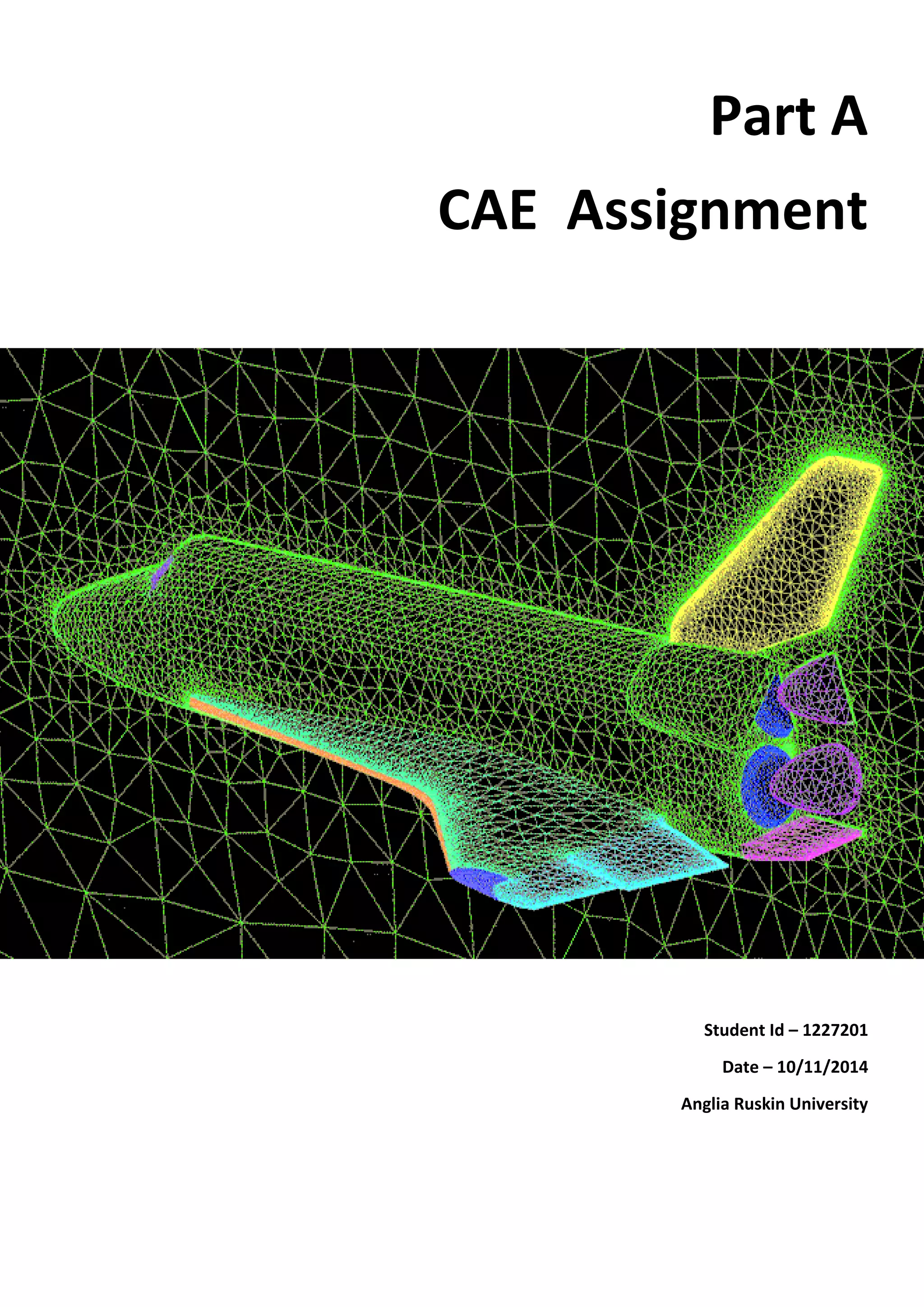
Introduction of CAE assignment for a student at Anglia Ruskin University, with student ID and date.
Outline of the workbook content including parts and exercises along with references and appendix.
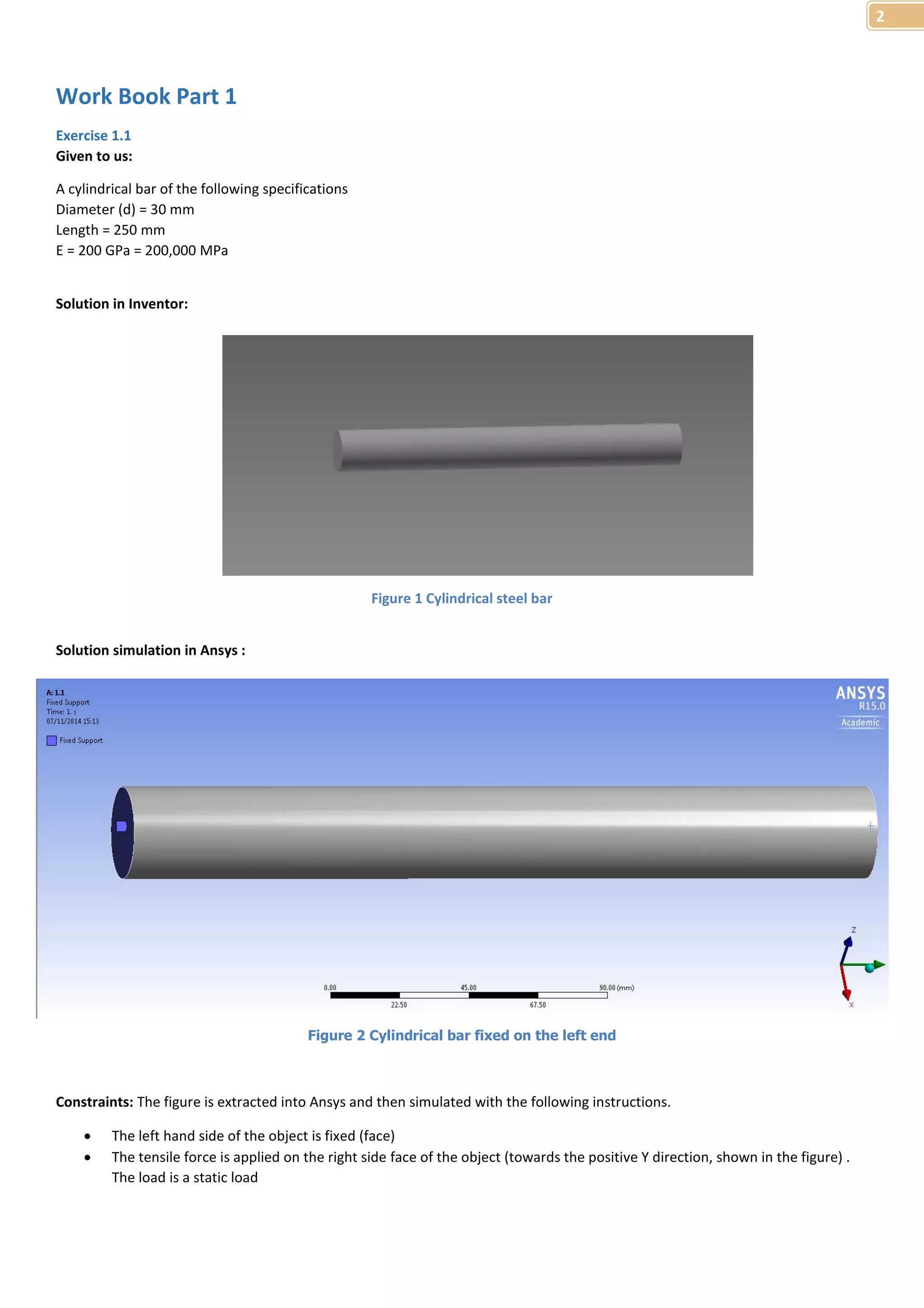
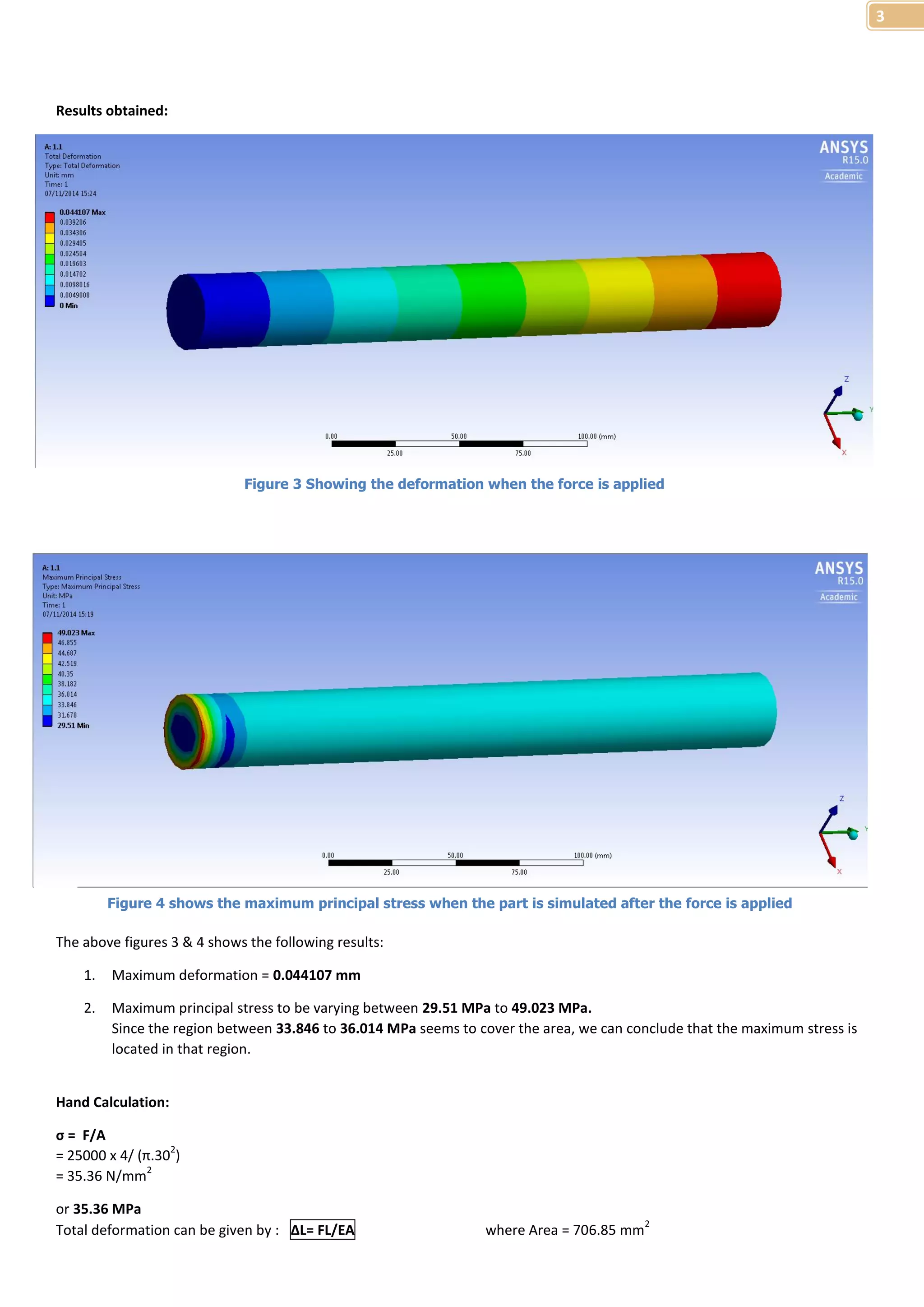
Analysis and simulation of a cylindrical bar subjected to tensile stress using Inventor and Ansys.
FEA results for a cantilever beam subjected to a load, showcasing stress and deformation calculations.
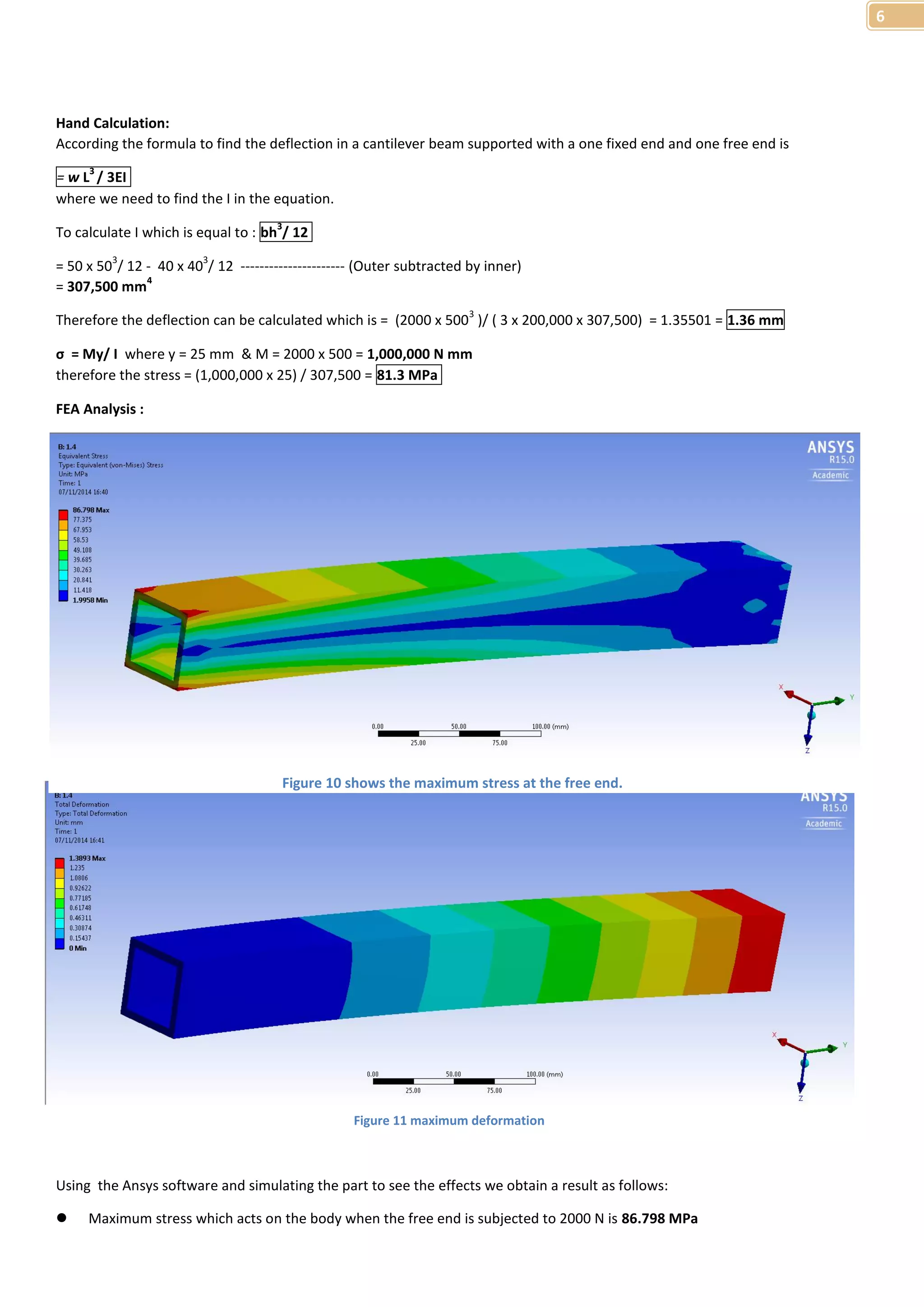
Detailed analysis of a hollow cantilever beam and comparison of hand calculations with FEA results.
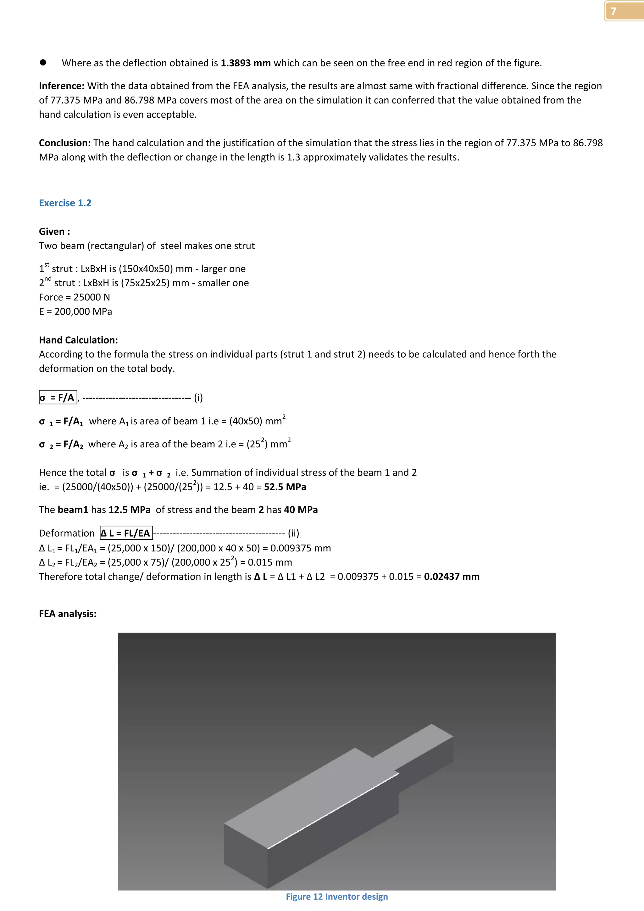
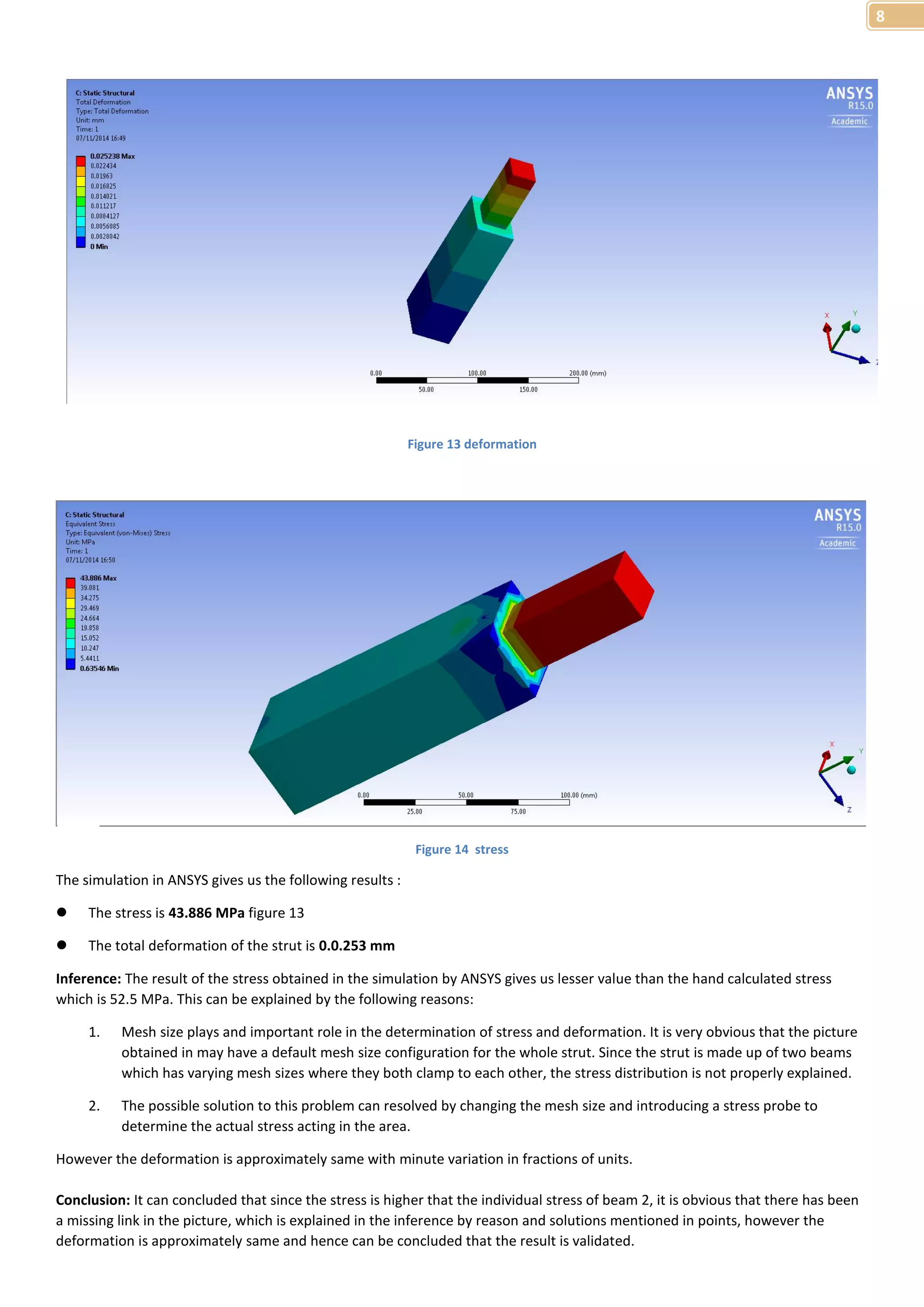
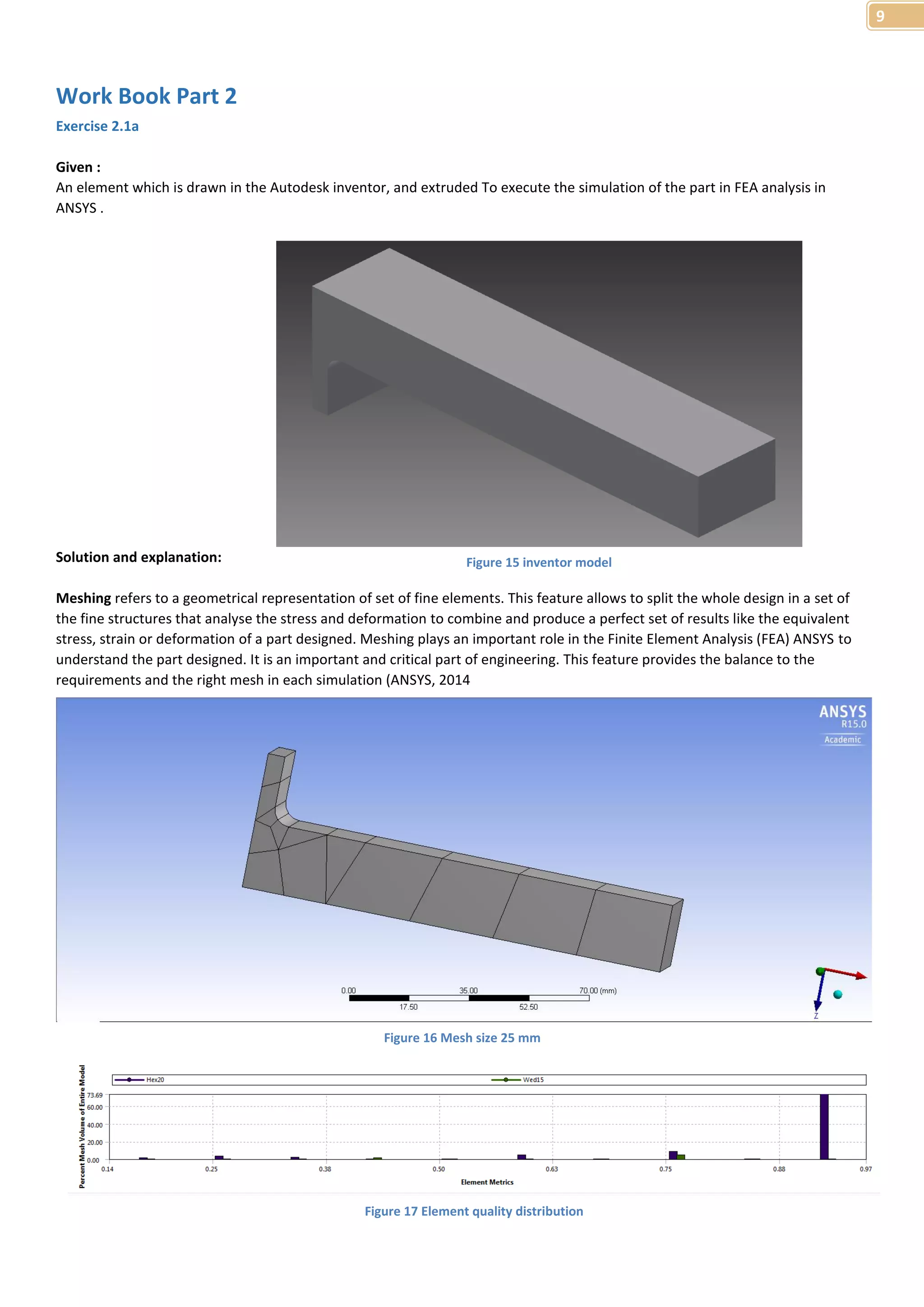
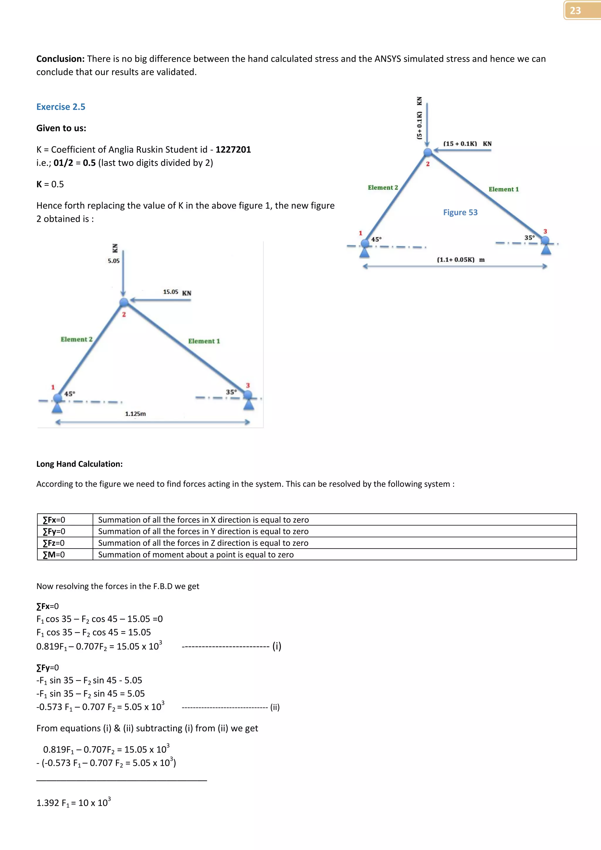
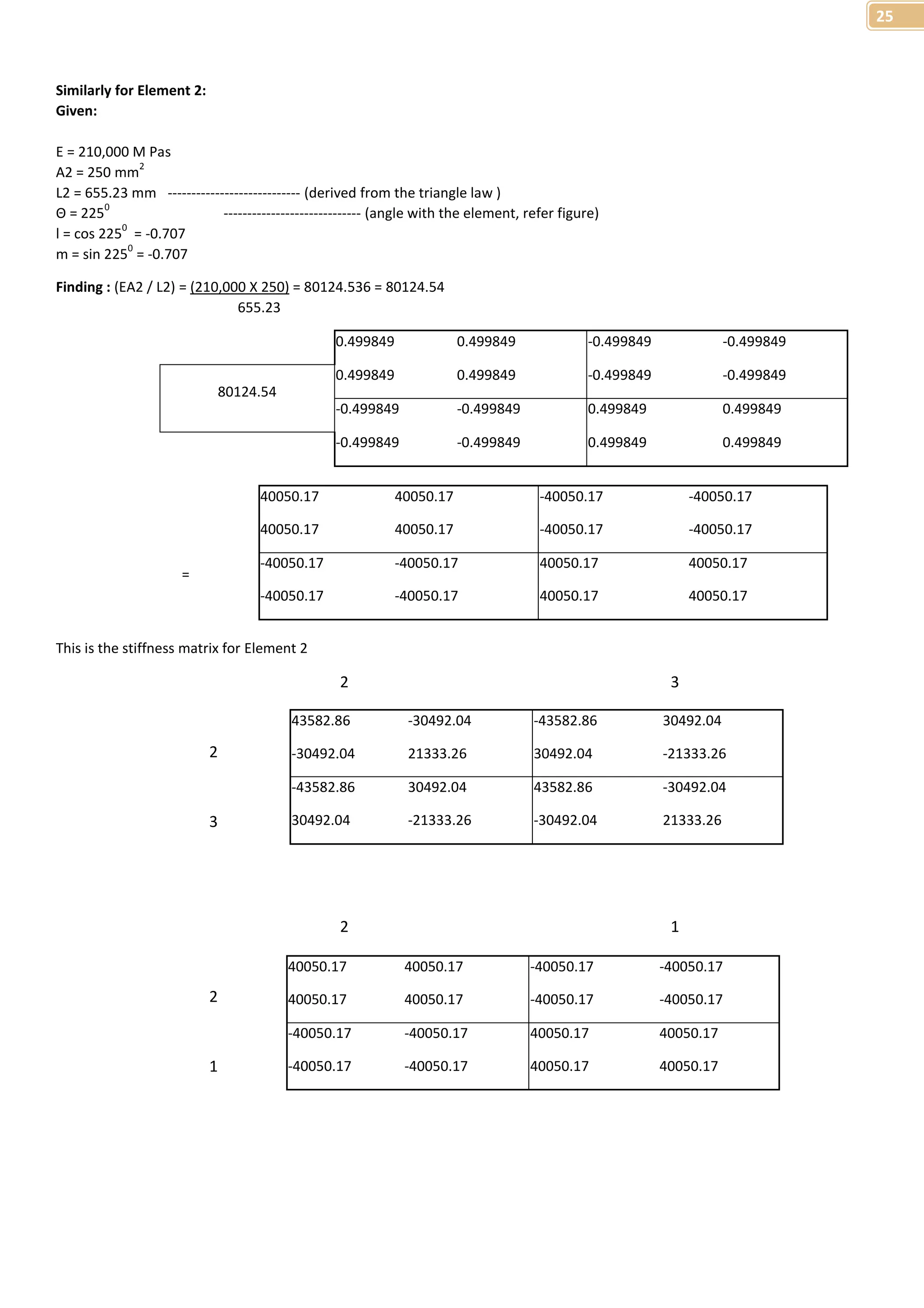
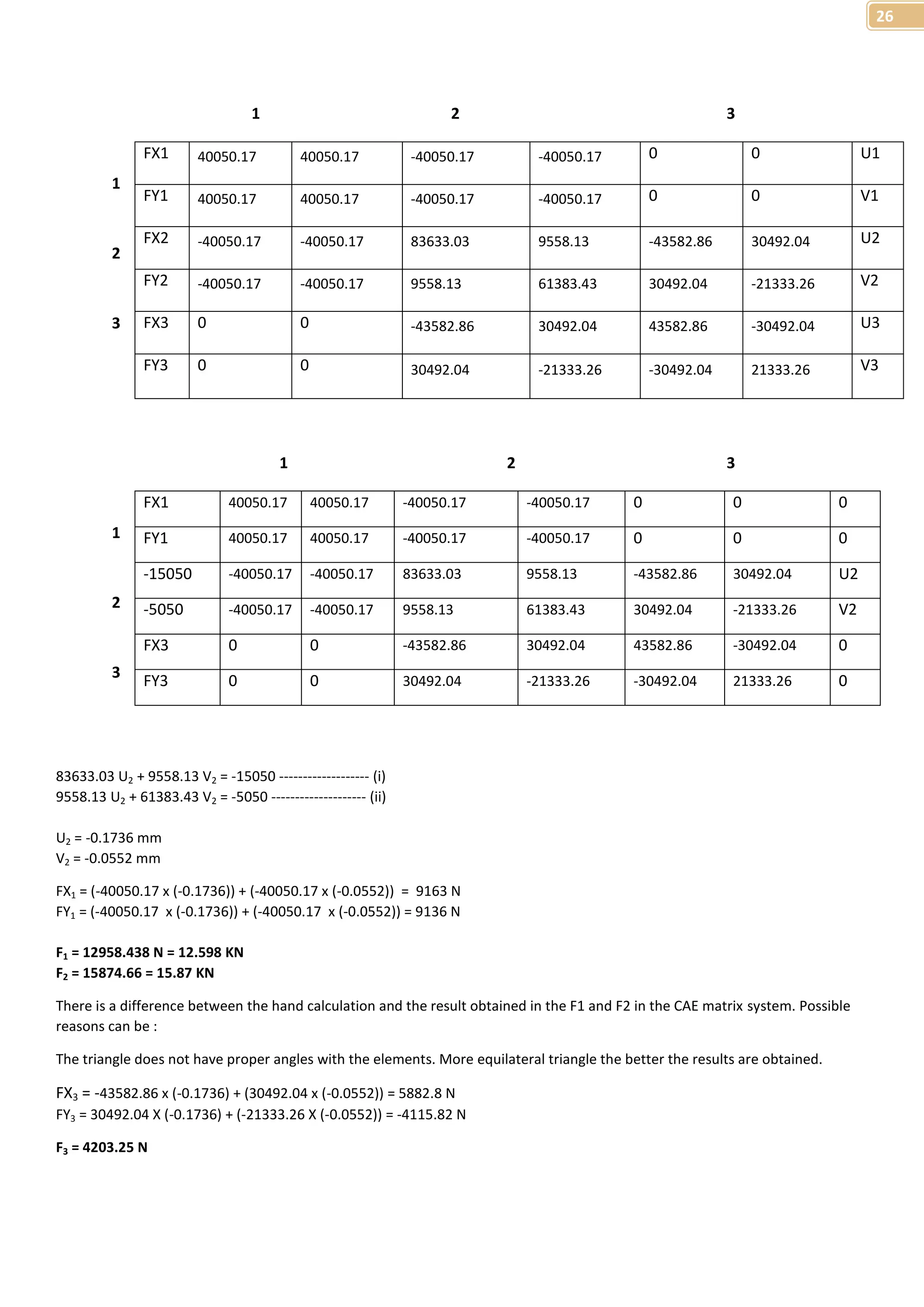
Calculates stress and deformation on two steel struts under load and compares hand calculations to FEA.
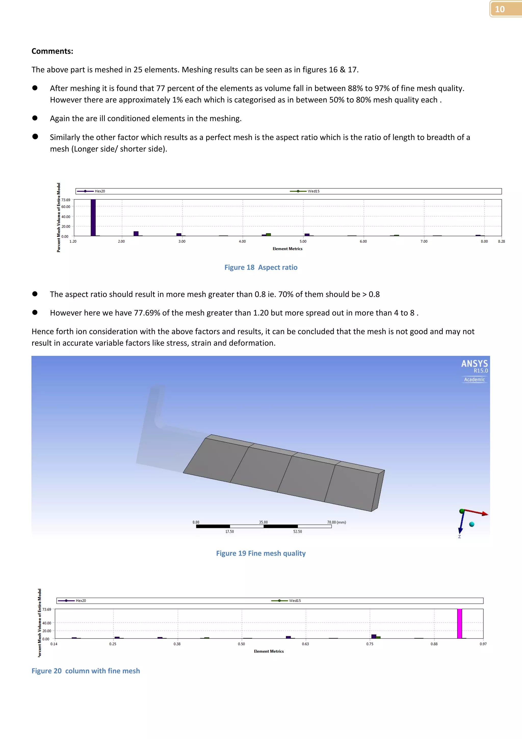
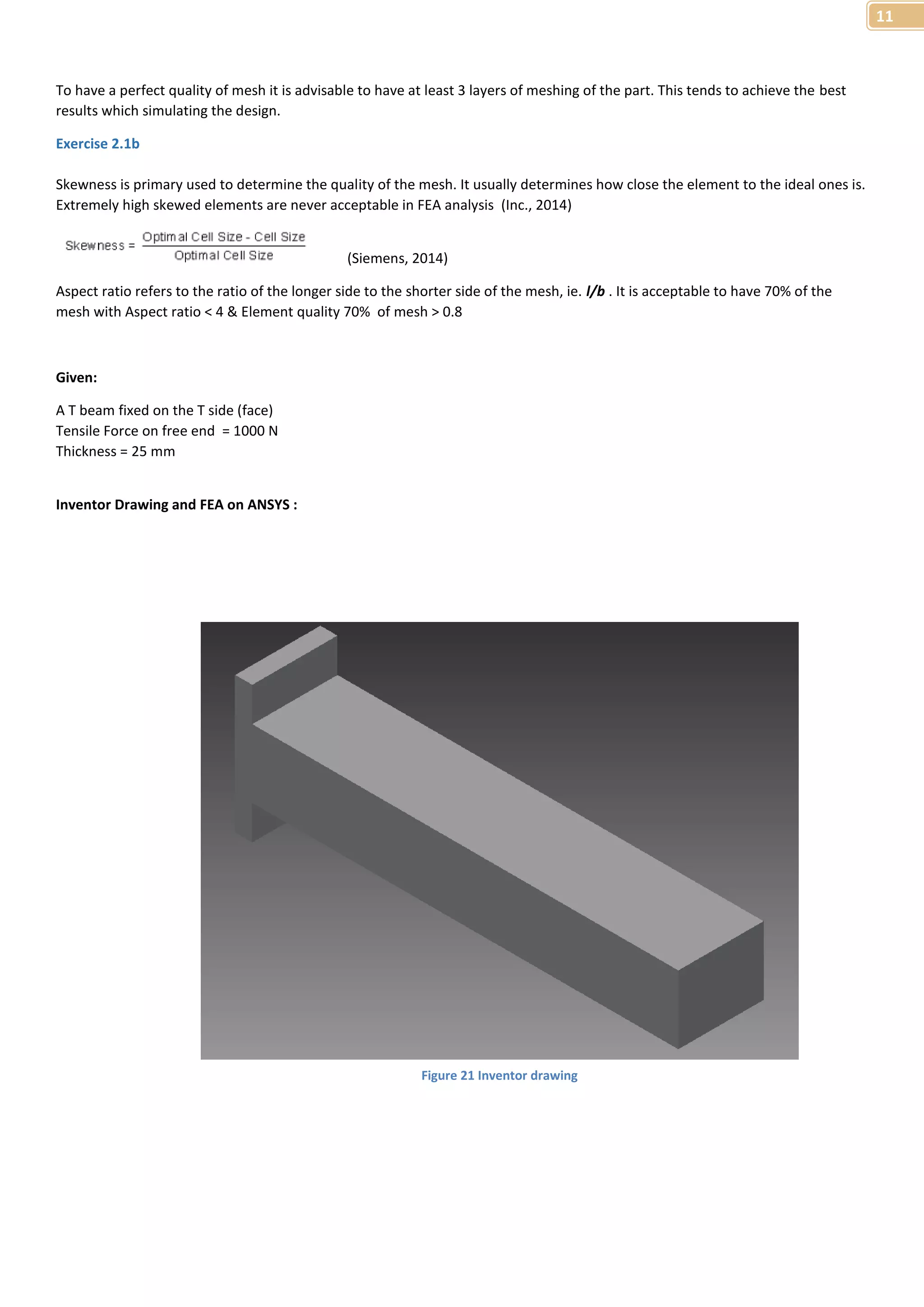
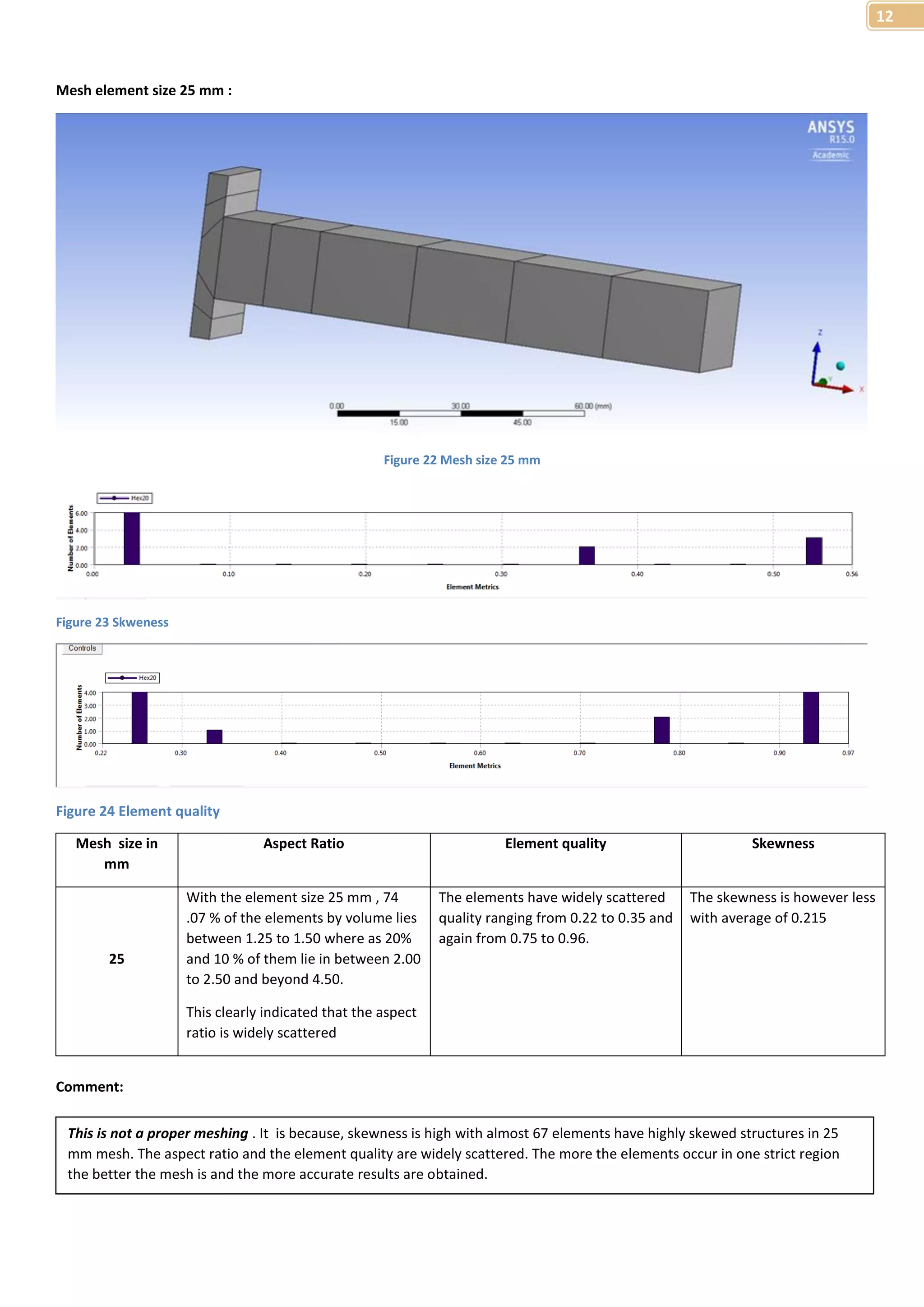
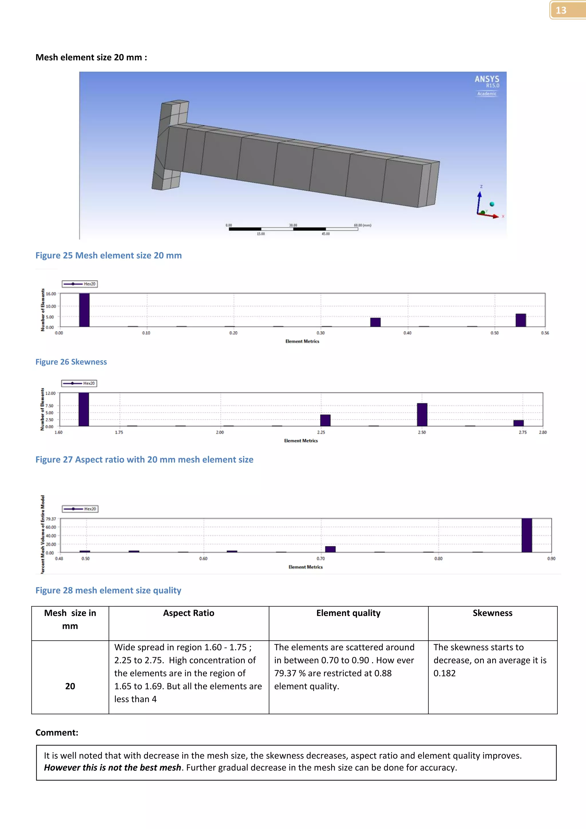
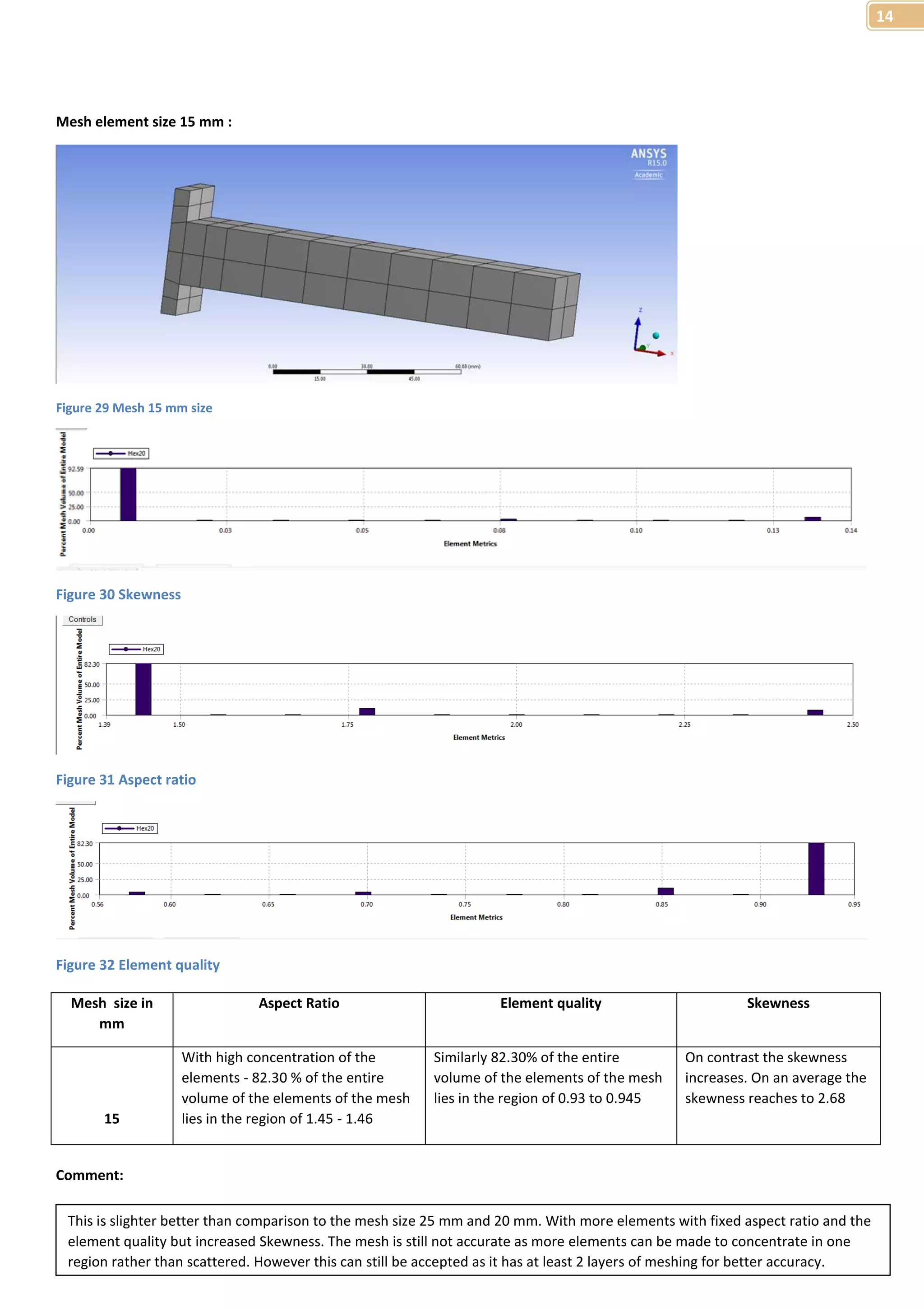
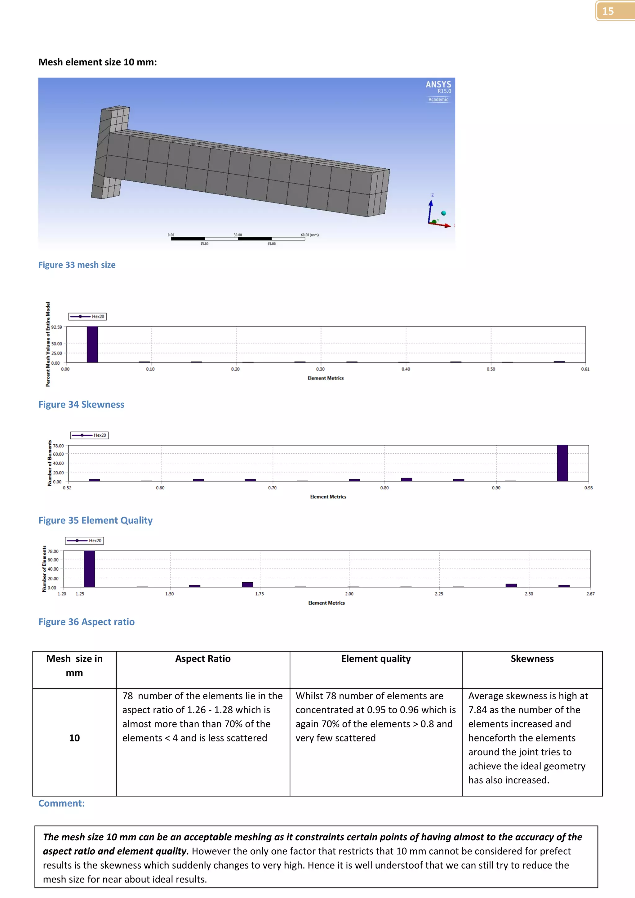
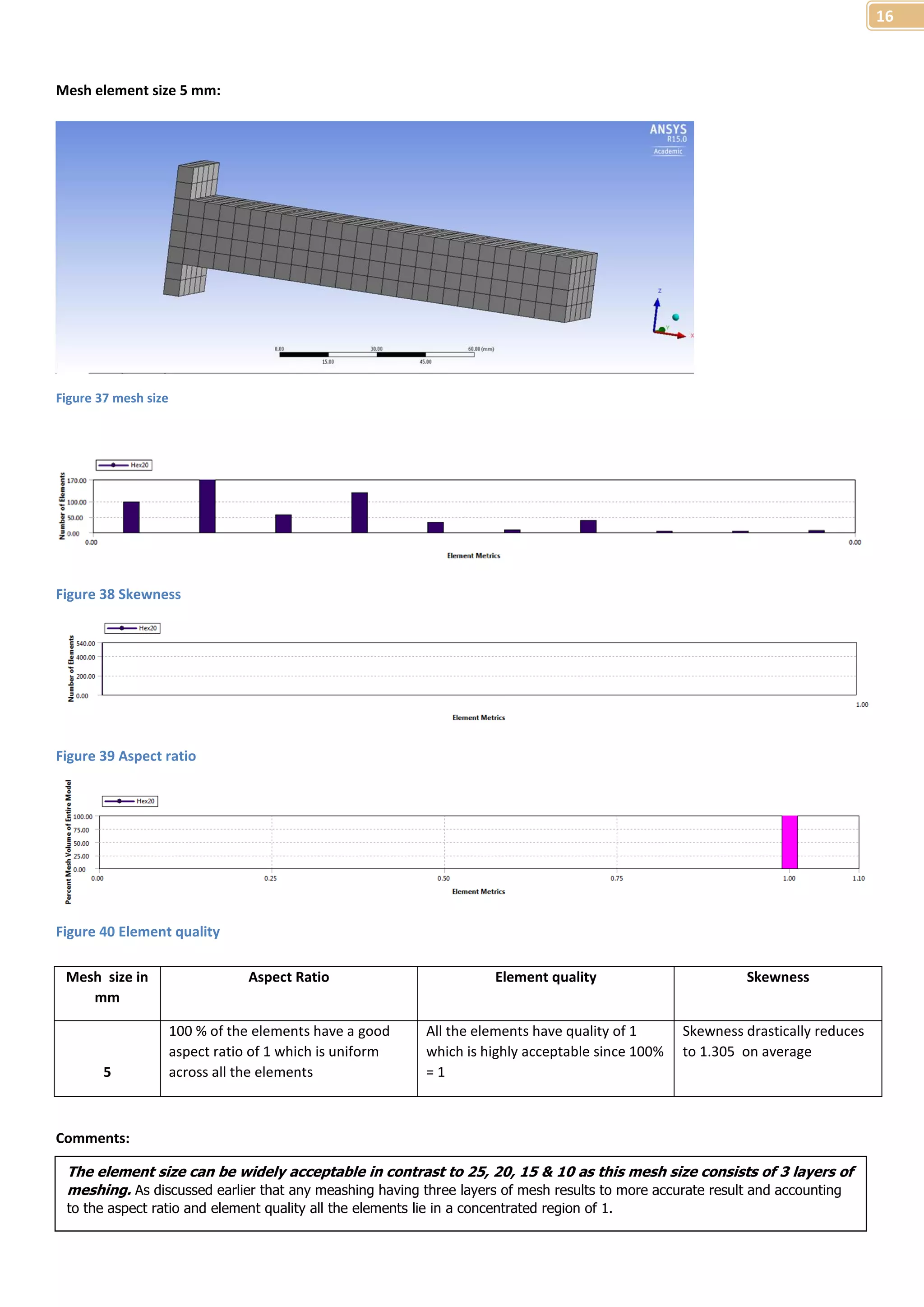
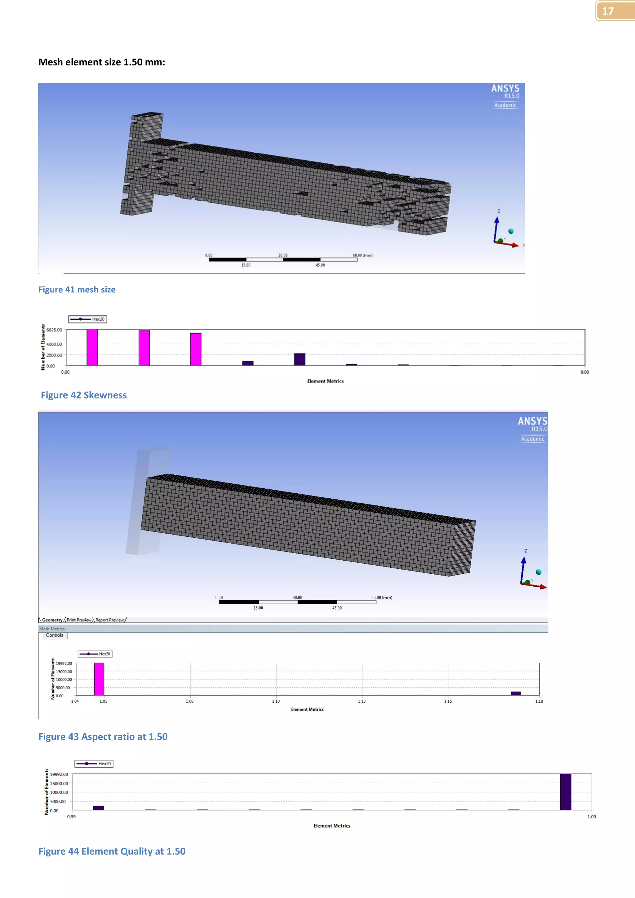
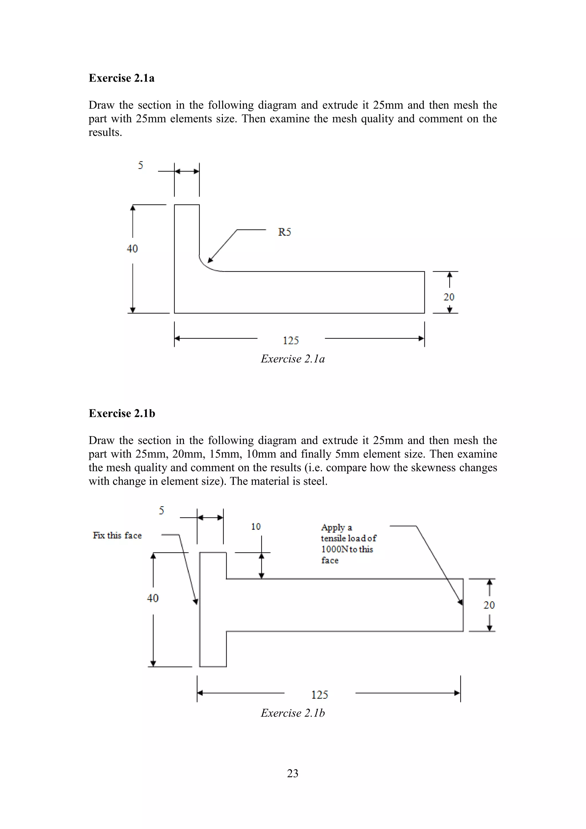
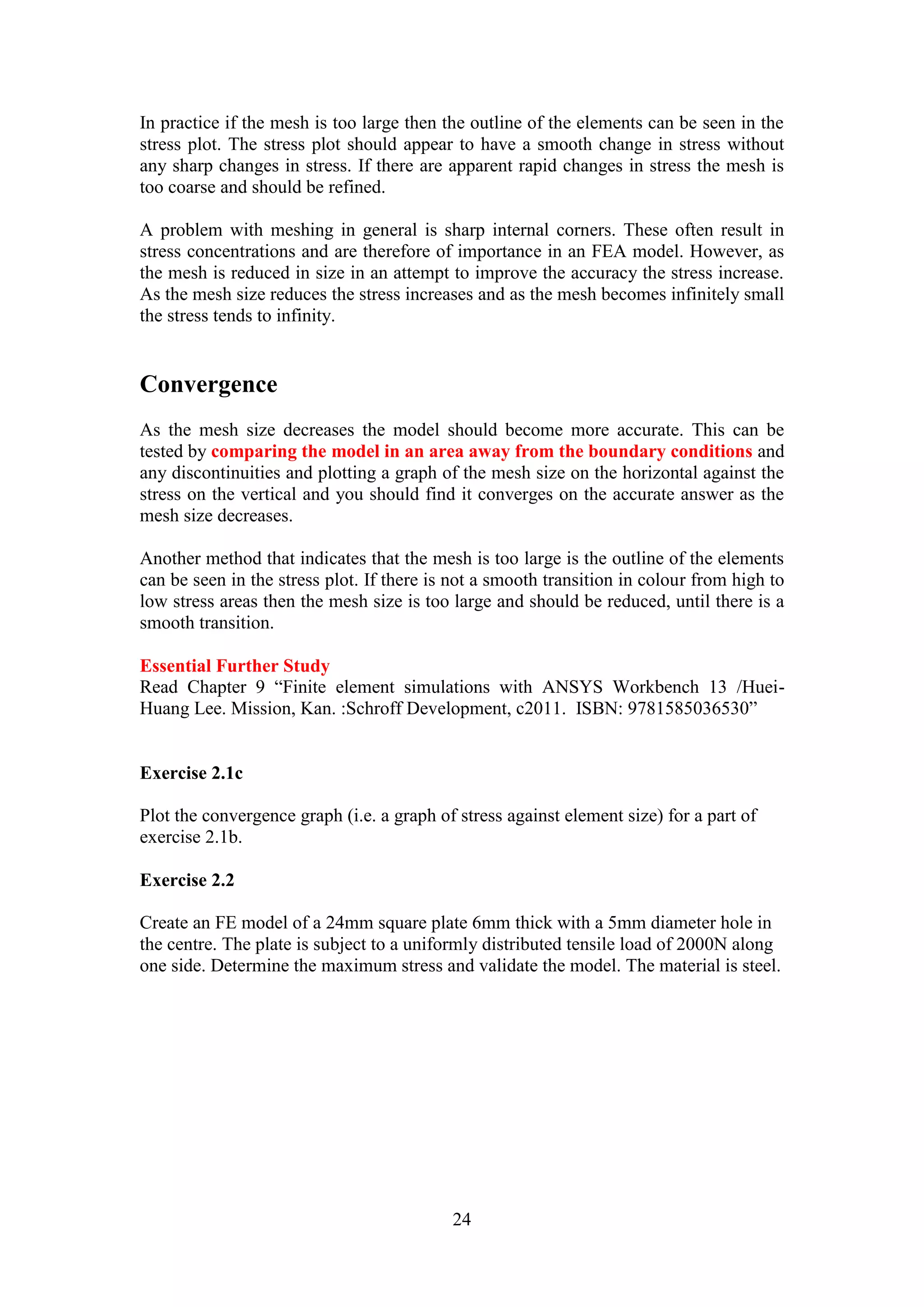
Overview of meshing processes in FEA and assessment of the mesh quality in an Autodesk Inventor model.
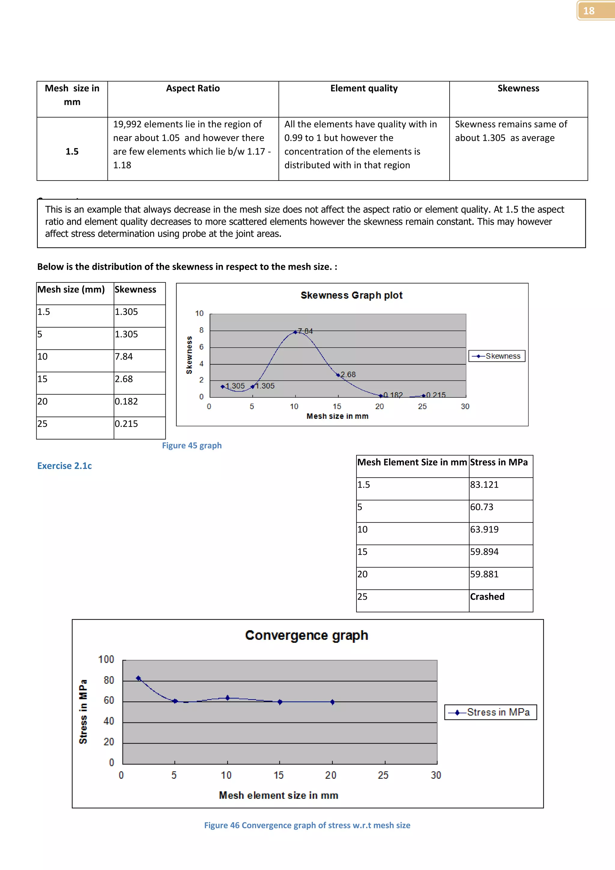
Evaluation of different mesh sizes (25mm to 5mm) and their effects on mesh quality using skewness.
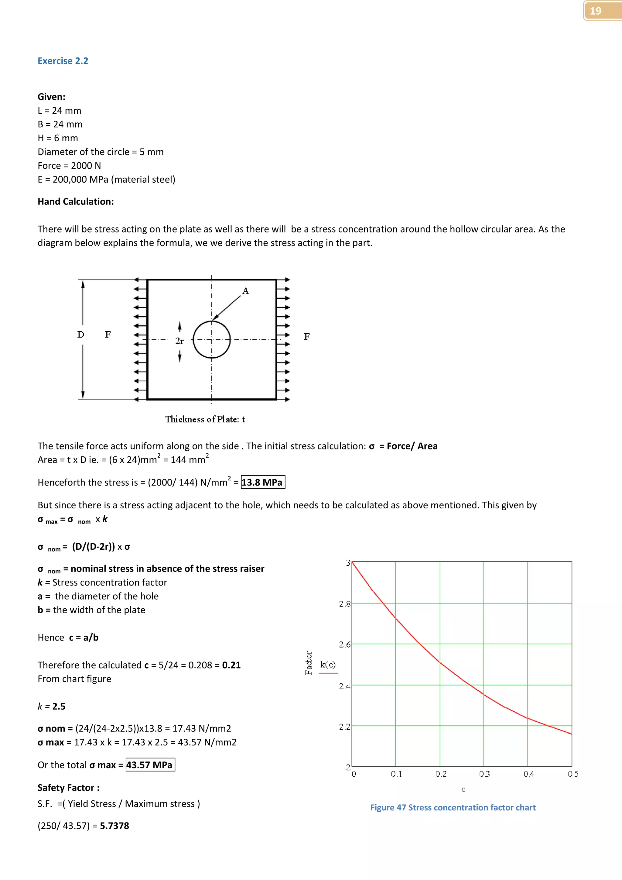
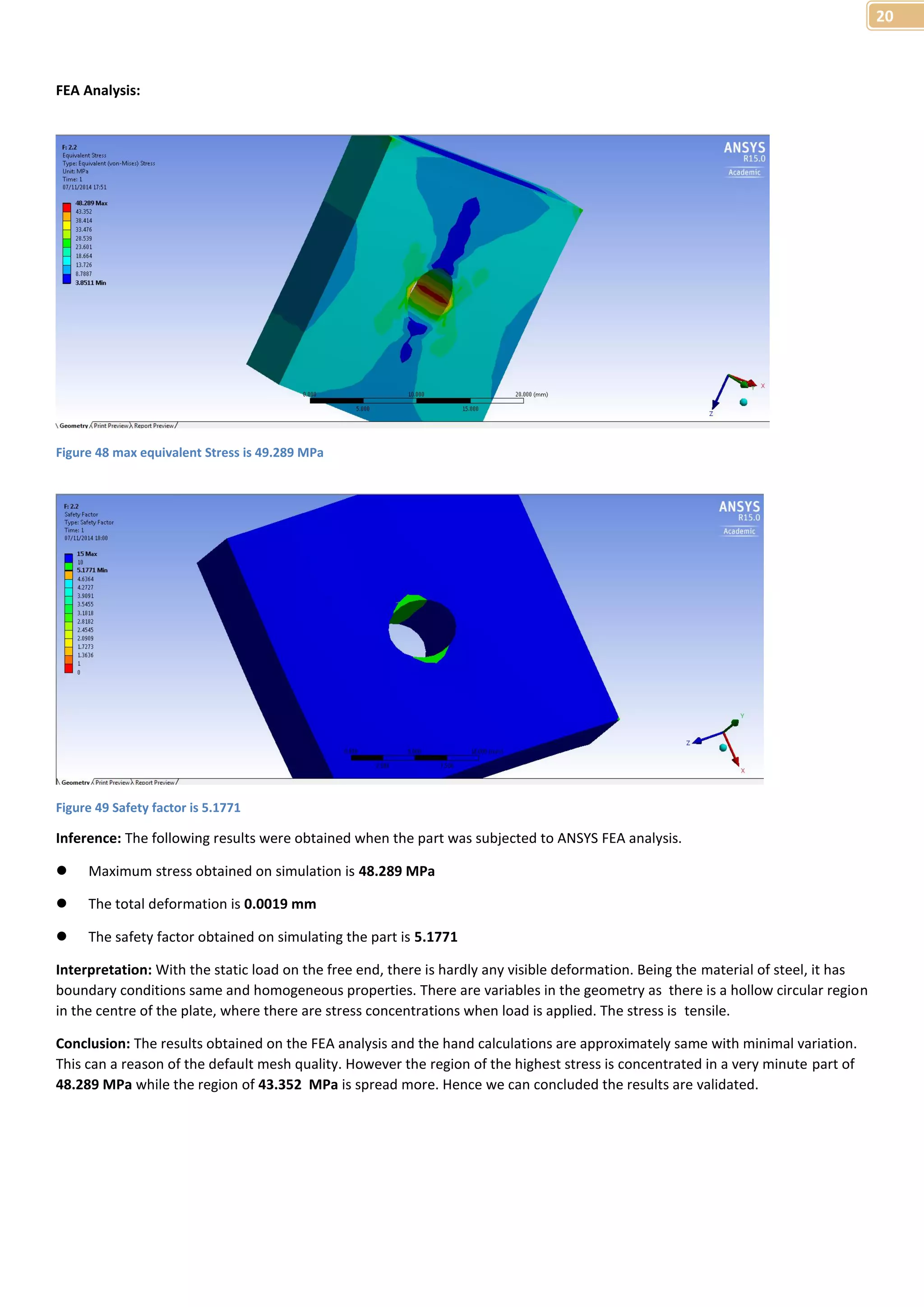
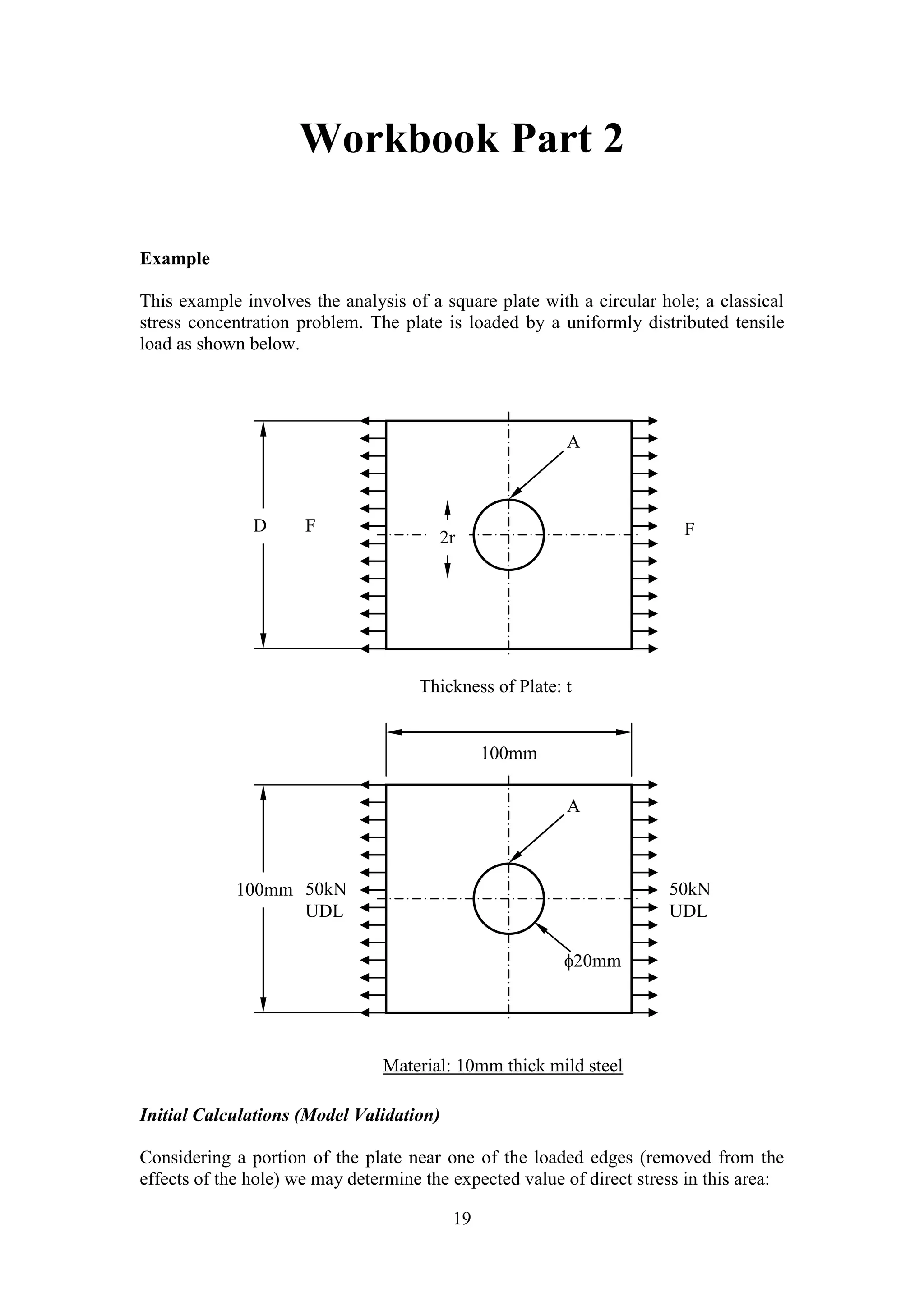
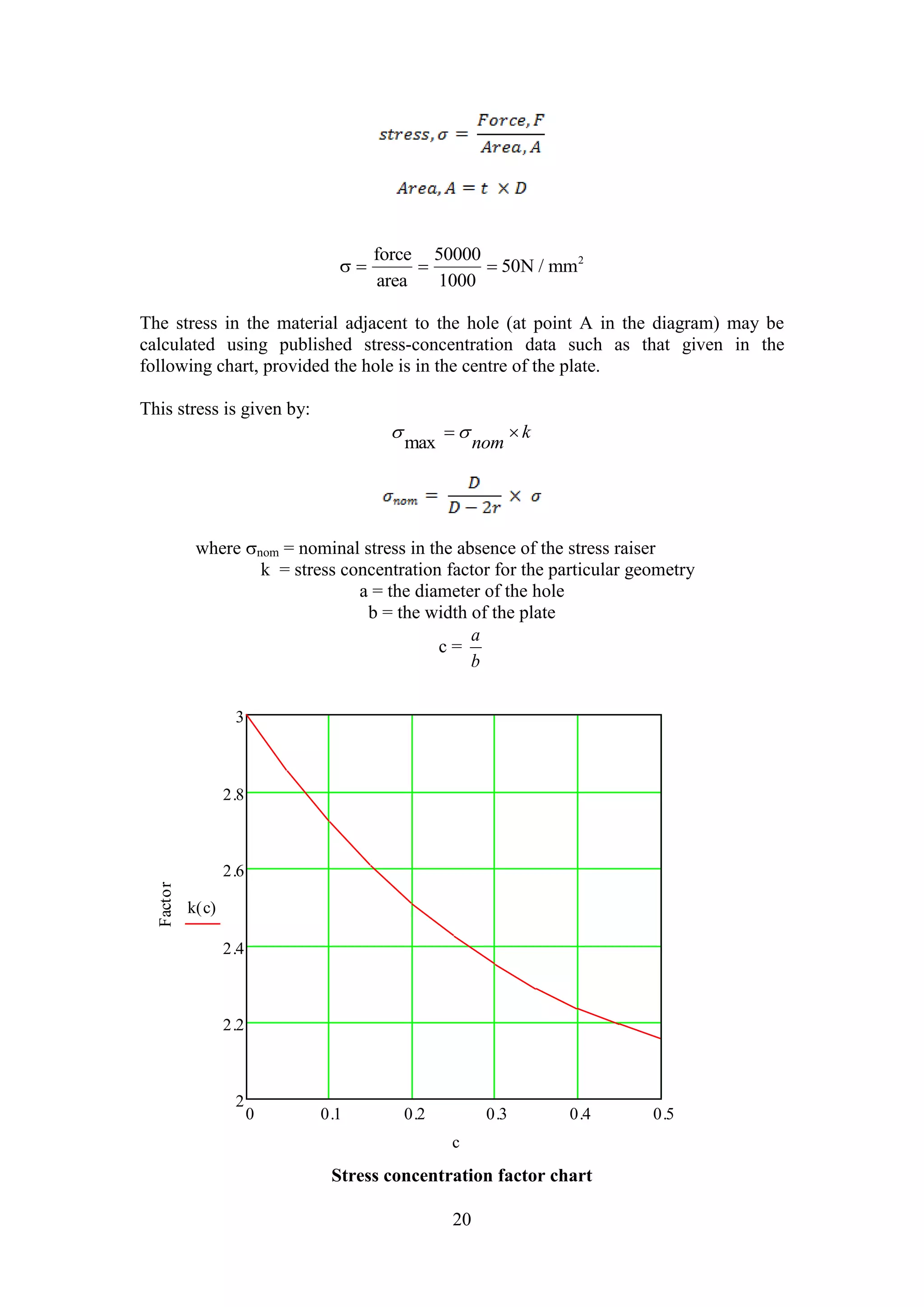
Calculations for stress concentration around a hole in a rectangular steel plate subjected to tensile load.
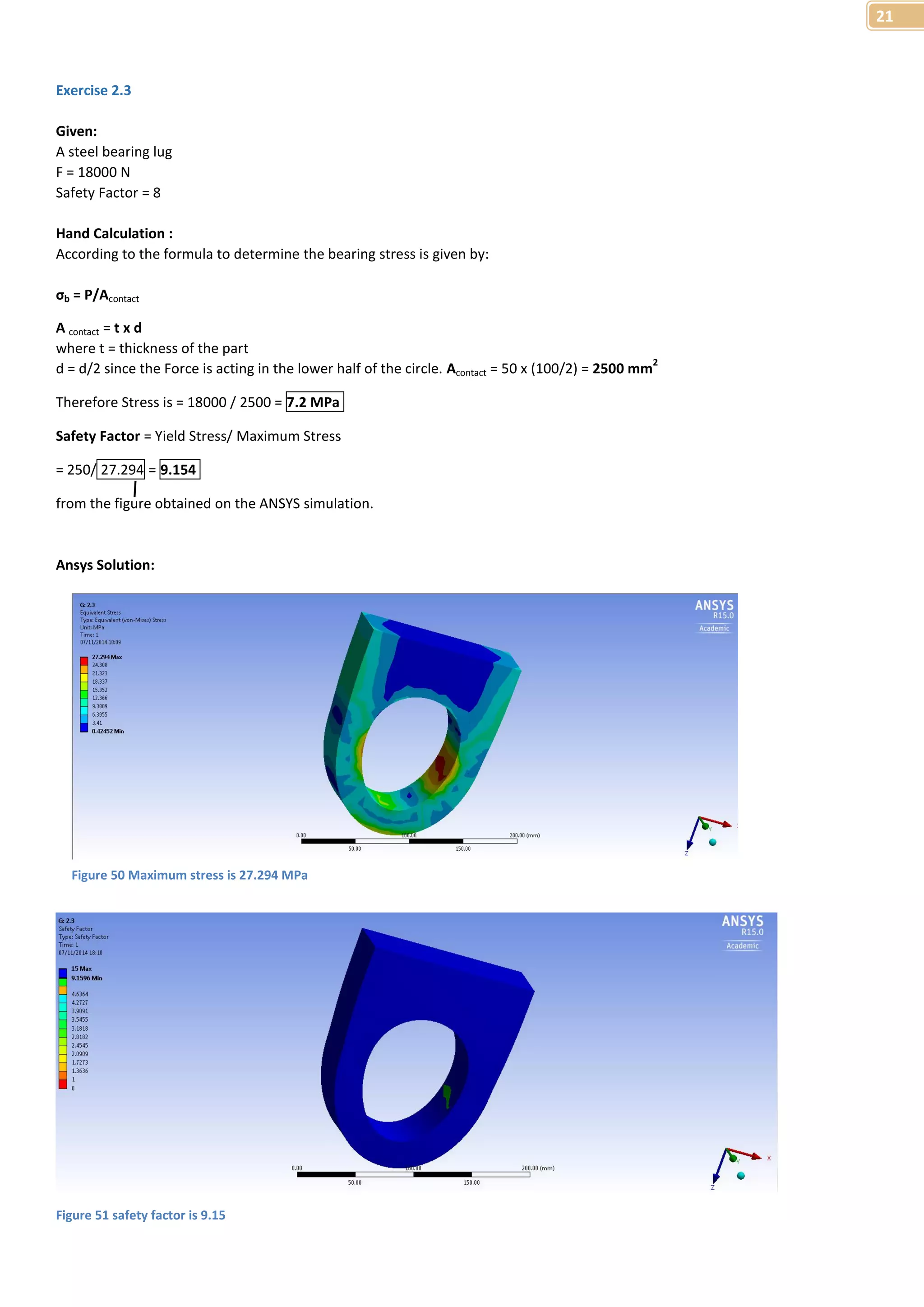
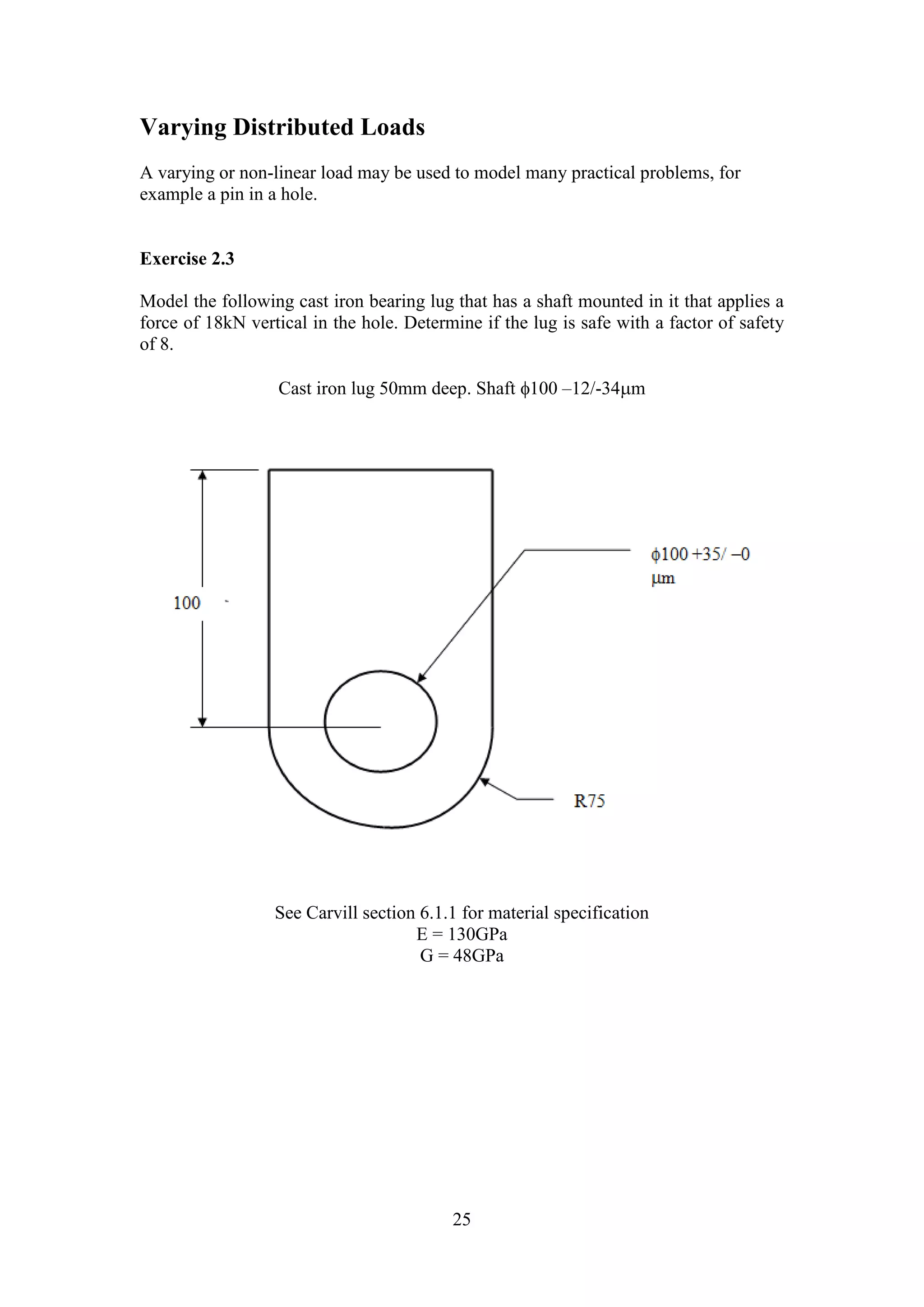
Assessment of bearing stress in a lug using hand calculations and FEA results with safety factor analysis.
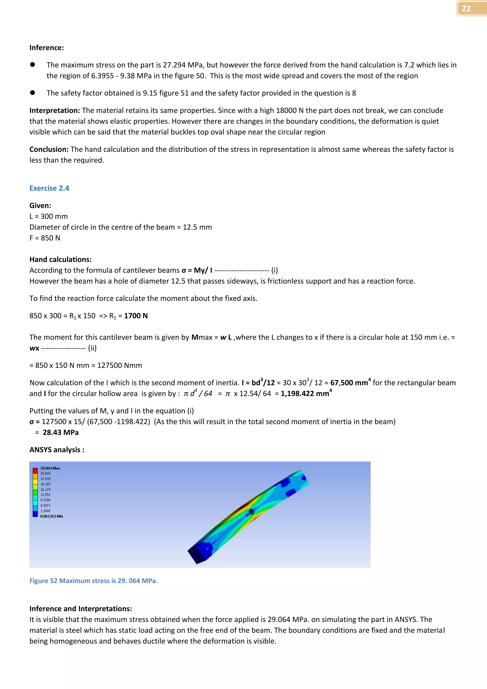
Analysis of stresses in a cantilever beam with a hole, comparing hand calculations to FEA simulations.
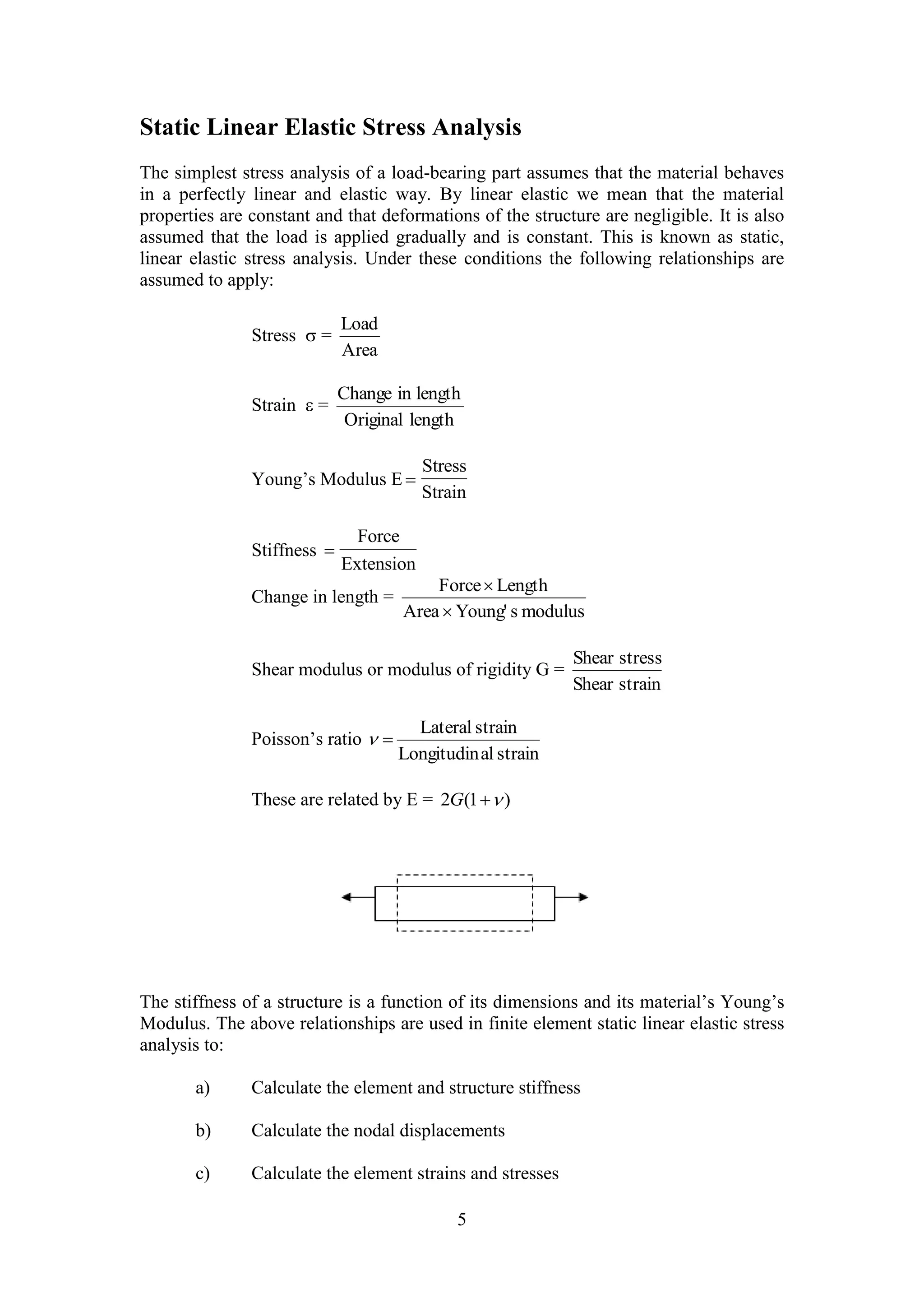
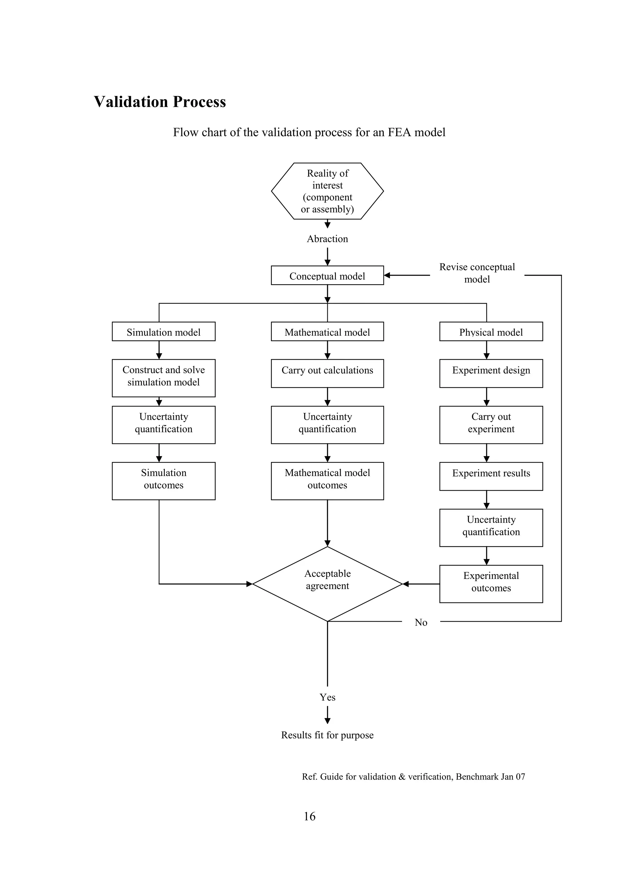
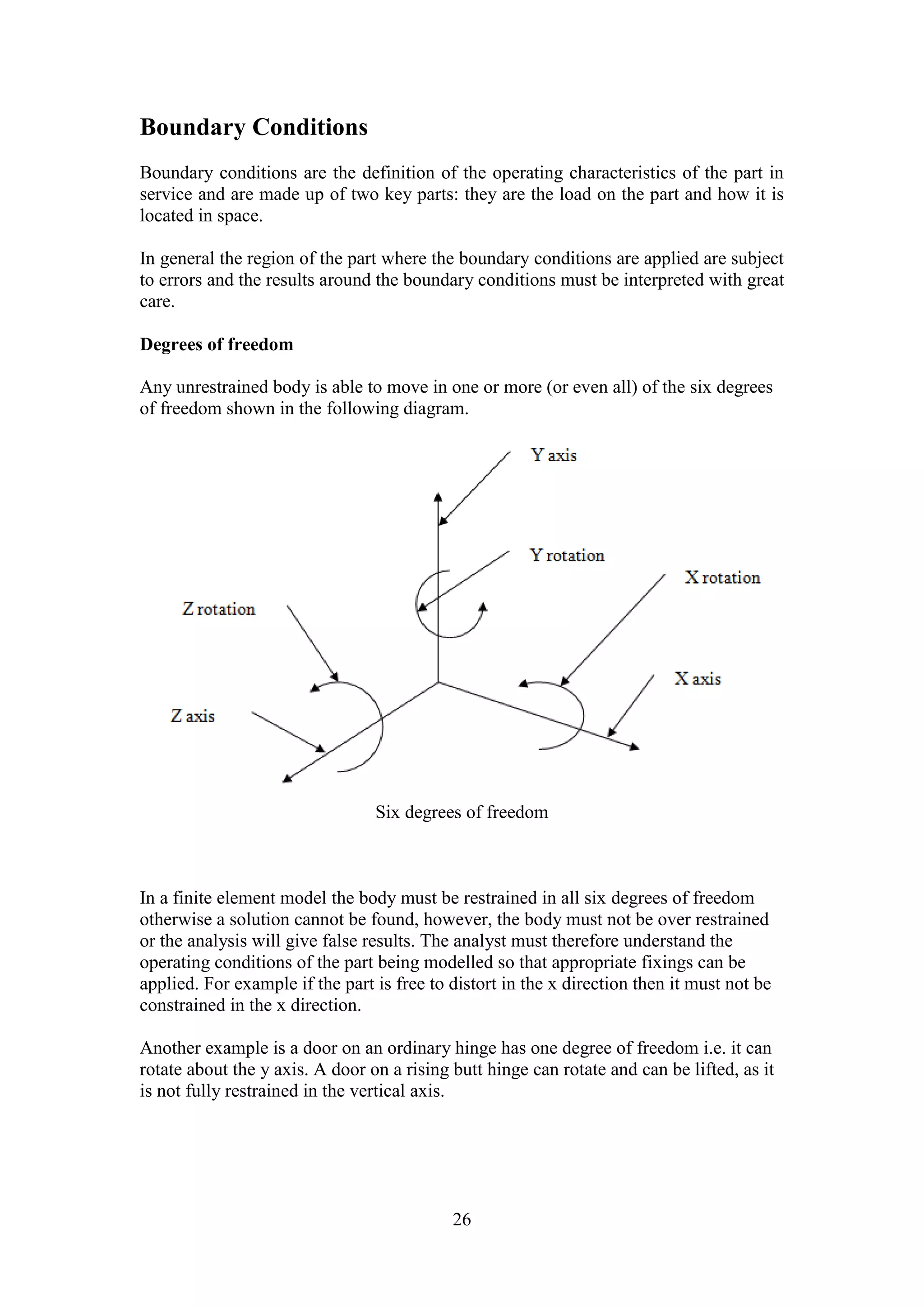
Validation of FE models, discussions on boundary conditions, and comprehensive finite element method guidelines.
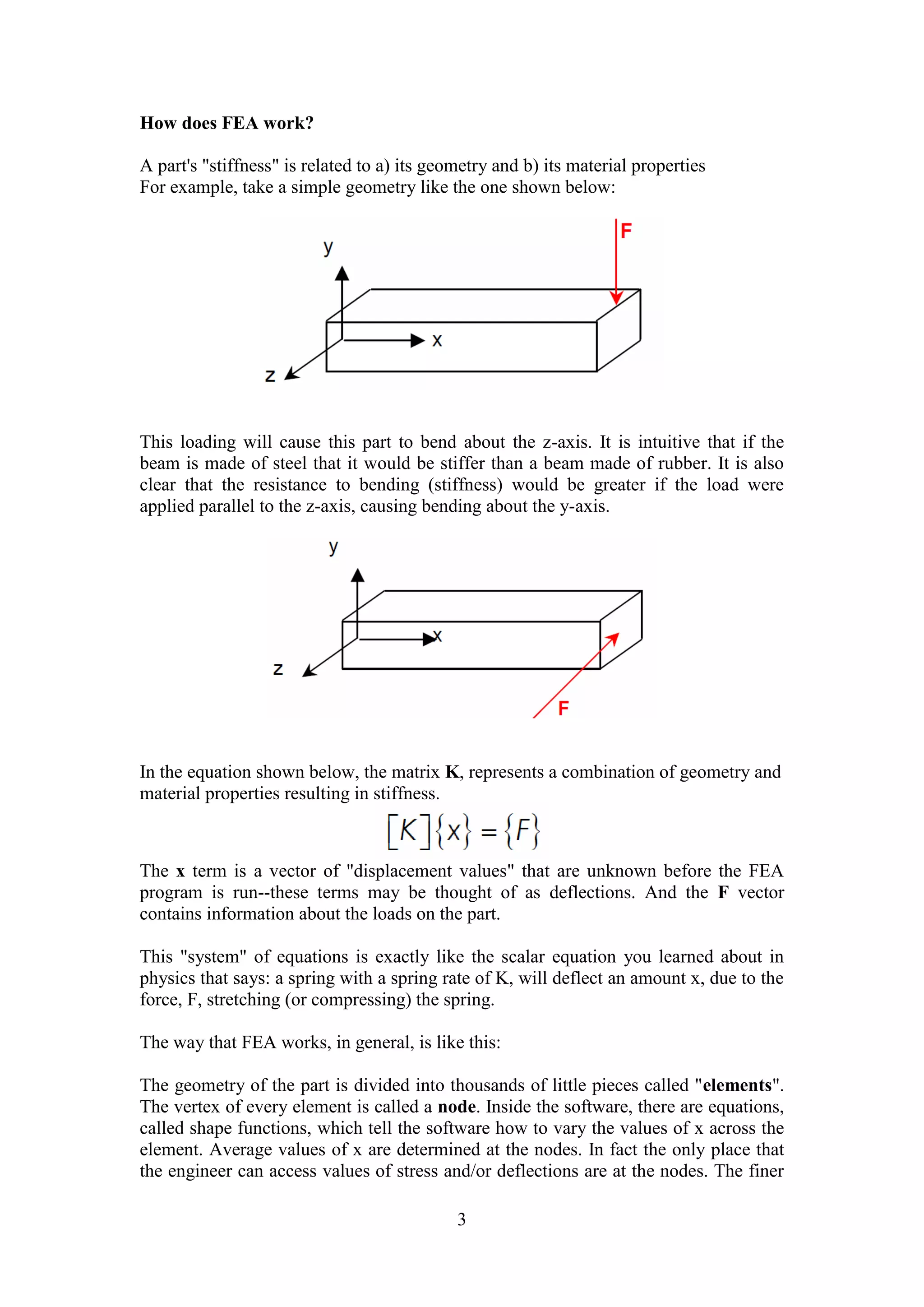
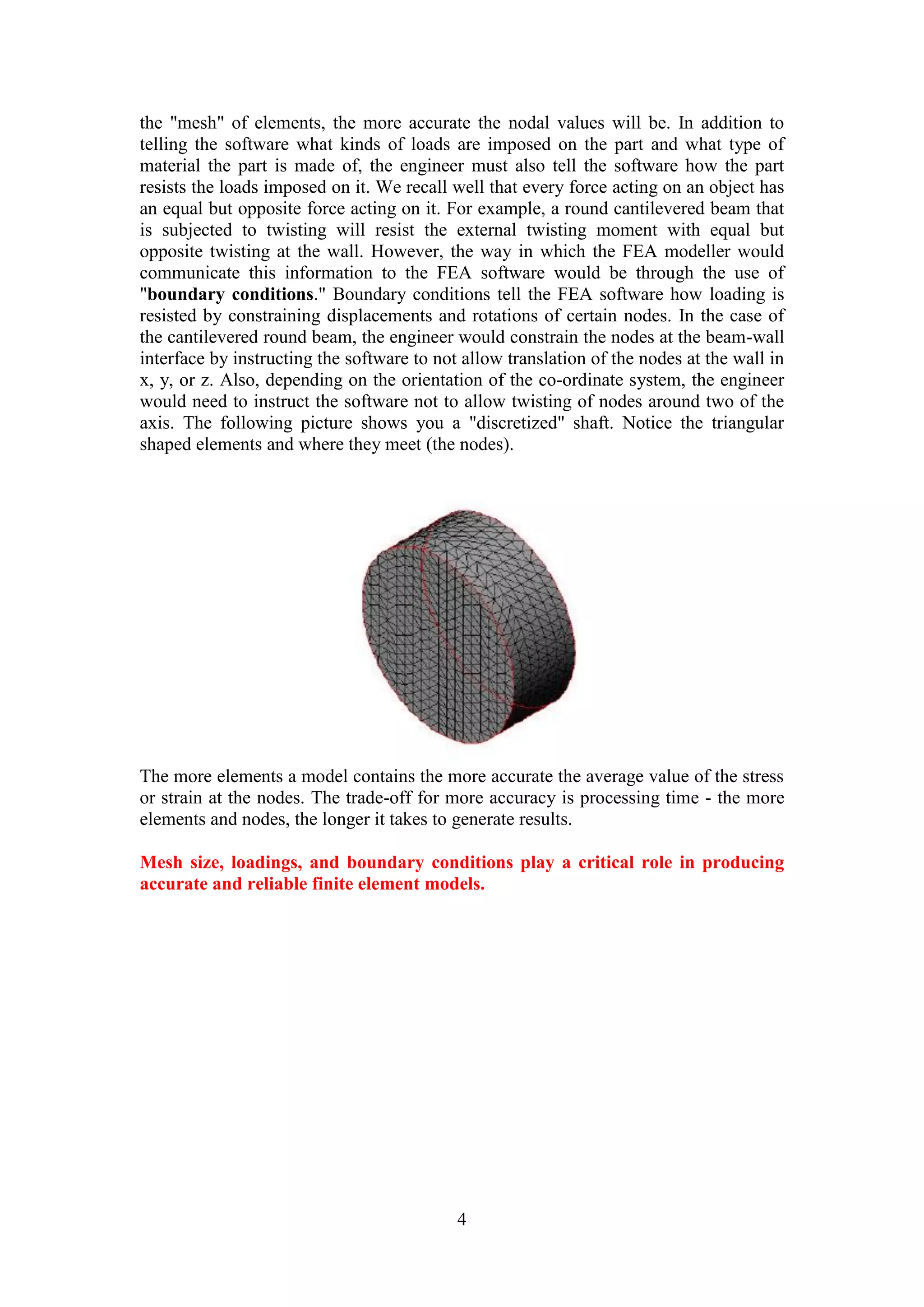
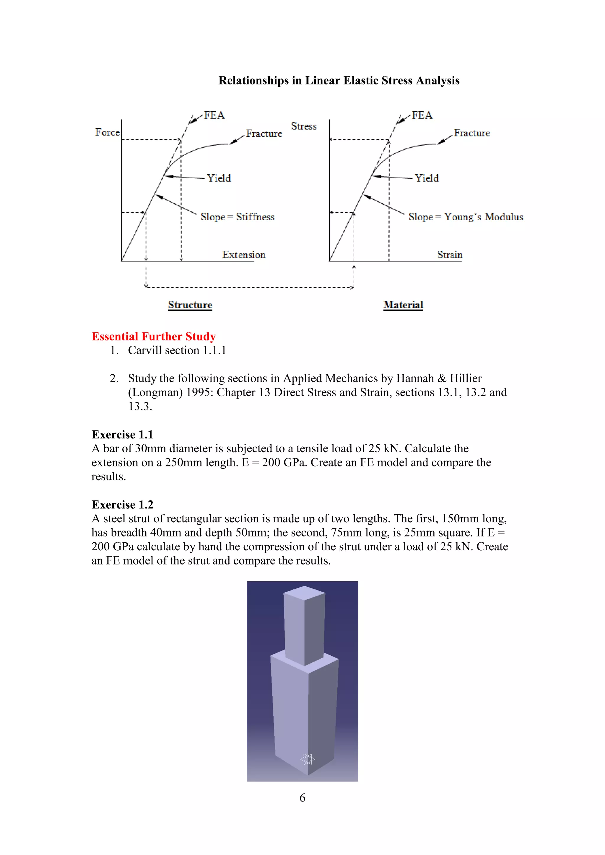
An overview of finite element analysis applications, outlining essential theory, calculations, and relationships.
Key questions for validating FEA results, material failure theories, and considerations in safety factor evaluations.
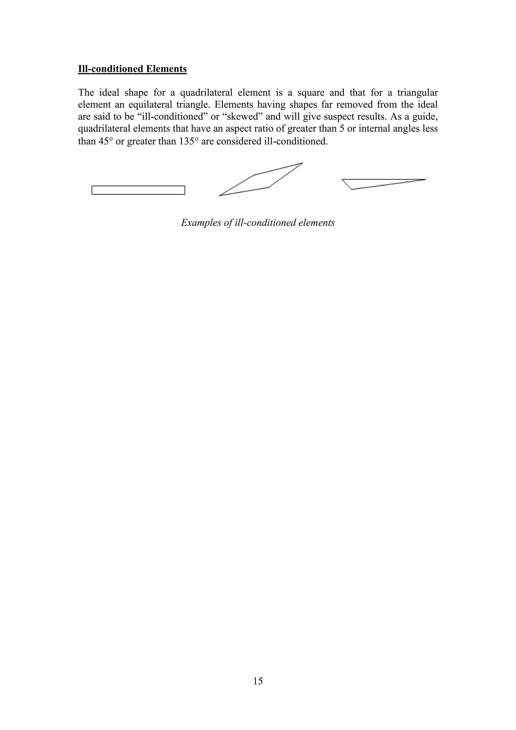
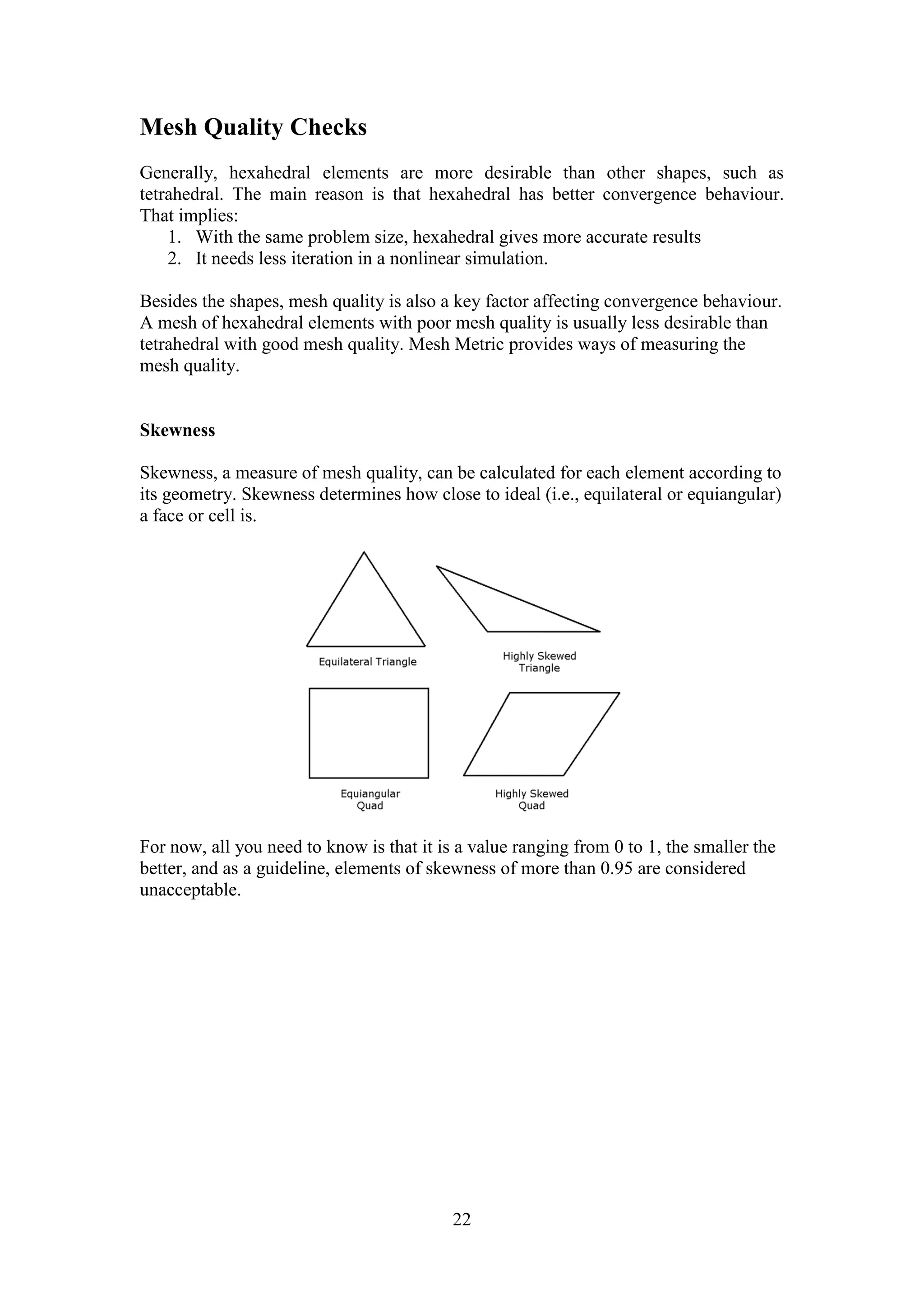
Recommendations for mesh quality checks, guidelines for convergence, and various computational exercises in FEA.
2
Work BookPart 1
Exercise 1.1
Given to us:
A cylindrical bar of the following specifications
Diameter (d) = 30 mm
Length = 250 mm
E = 200 GPa = 200,000 MPa
Solution in Inventor:
Figure 1 Cylindrical steel bar
Solution simulation in Ansys :
Constraints: The figure is extracted into Ansys and then simulated with the following instructions.
The left hand side of the object is fixed (face)
The tensile force is applied on the right side face of the object (towards the positive Y direction, shown in the figure) .
The load is a static load
Figure 2 Cylindrical bar fixed on the left end
4.
3
Results obtained:
Figure 3 Showing the deformation when the force is applied
Figure 4 shows the maximum principal stress when the part is simulated after the force is applied
The above figures 3 & 4 shows the following results:
1. Maximum deformation = 0.044107 mm
2. Maximum principal stress to be varying between 29.51 MPa to 49.023 MPa.
Since the region between 33.846 to 36.014 MPa seems to cover the area, we can conclude that the maximum stress is
located in that region.
Hand Calculation:
σ = F/A
= 25000 x 4/ (π.302)
= 35.36 N/mm2
or 35.36 MPa
Total deformation can be given by : ΔL= FL/EA where Area = 706.85 mm2
5.
4
= (25000X 250 ) / (200,000 X 706.85)
= 0.044210 mm
Interference: The result obtained on the Long hand calculation and the result from the Ansys FEA coincides with the long hand
calculation as the deformation is at the most same and the region of the maximum stress lies same result obtained on the hand
calculation.
Exercise 1.3
Given to us:
Steel Cantilever beam
L = 250 mm
b = 20 mm
h = 40 mm
E = 200 000 MPa
Load = 2000 N
Hand calculation:
formula give to us for deflection is : w L3 / 3EI but to calculate deflection we need to find I .
Formula for I = bh3/ 12
i.e = ( 20 x 403 )/ 12 = 106,666.6 mm4
therefore the deflection is = (2000 x 2503) / (3 x 200,000 x 106,666.6)
= 0.488 mm
σ = My / I -------------------------------------------- (1)
M= 2000 x 250 = 500,000 Nm ------------------------------- (2)
Putting the value of 2 in 1 we get
σ = (500,000 x 20) / 106,666.6 = 93.75 MPa
Figure 5 shows the steel cantilever beam in inventor
Figure 6 showing the maximum and minimum stress acting on the cantilever beam
6.
5
From theabove figures 6 & 7 it can be seen that the part has been FEA analyzed and that the following interference can be
made:
The maximum stress when the part is fixed on one end and subjected to tensile force of 2000 N on the free end, results in a
maximum of 95.309 MPa.
On the same analysis for the deformation in FEA, it results to be 0.49725 mm
Inference: We can conclude that the result obtained in the hand calculation and the results obtained from the FEA analysis of
the part shows a very minute or fraction difference in the figure however they are accurate to certain extent.
Conclusion: It can established that the results are validated with the hand calculation.
Exercise 1.4
Given to us :
Outer square = 50 mm
Inner Square = 40 mm
Extrude/ Length = 500 mm
Load = 200 Kg = 2,000 Newton
E= 200,000 MPa
Figure 7 shows the deformation on the cantilever beam
Figure 9 diagrammatic representation of the load and the fixed support.
Figure 8 hollow beam inventor
drawing
7.
6
Hand Calculation:
According the formula to find the deflection in a cantilever beam supported with a one fixed end and one free end is
= w L3 / 3EI
where we need to find the I in the equation.
To calculate I which is equal to : bh3/ 12
= 50 x 503/ 12 - 40 x 403/ 12 ---------------------- (Outer subtracted by inner)
= 307,500 mm4
Therefore the deflection can be calculated which is = (2000 x 5003 )/ ( 3 x 200,000 x 307,500) = 1.35501 = 1.36 mm
σ = My/ I where y = 25 mm & M = 2000 x 500 = 1,000,000 N mm
therefore the stress = (1,000,000 x 25) / 307,500 = 81.3 MPa
FEA Analysis :
Figure 10 shows the maximum stress at the free end.
Figure 11 maximum deformation
Using the Ansys software and simulating the part to see the effects we obtain a result as follows:
Maximum stress which acts on the body when the free end is subjected to 2000 N is 86.798 MPa
8.
7
Whereas the deflection obtained is 1.3893 mm which can be seen on the free end in red region of the figure.
Inference: With the data obtained from the FEA analysis, the results are almost same with fractional difference. Since the region
of 77.375 MPa and 86.798 MPa covers most of the area on the simulation it can conferred that the value obtained from the
hand calculation is even acceptable.
Conclusion: The hand calculation and the justification of the simulation that the stress lies in the region of 77.375 MPa to 86.798
MPa along with the deflection or change in the length is 1.3 approximately validates the results.
Exercise 1.2
Given :
Two beam (rectangular) of steel makes one strut
1st strut : LxBxH is (150x40x50) mm - larger one
2nd strut : LxBxH is (75x25x25) mm - smaller one
Force = 25000 N
E = 200,000 MPa
Hand Calculation:
According to the formula the stress on individual parts (strut 1 and strut 2) needs to be calculated and hence forth the
deformation on the total body.
σ = F/A , --------------------------------- (i)
σ 1 = F/A1 where A1 is area of beam 1 i.e = (40x50) mm2
σ 2 = F/A2 where A2 is area of the beam 2 i.e = (252) mm2
Hence the total σ is σ 1 + σ 2 i.e. Summation of individual stress of the beam 1 and 2
ie. = (25000/(40x50)) + (25000/(252)) = 12.5 + 40 = 52.5 MPa
The beam1 has 12.5 MPa of stress and the beam 2 has 40 MPa
Deformation Δ L = FL/EA ---------------------------------------- (ii)
Δ L1 = FL1/EA1 = (25,000 x 150)/ (200,000 x 40 x 50) = 0.009375 mm
Δ L2 = FL2/EA2 = (25,000 x 75)/ (200,000 x 252) = 0.015 mm
Therefore total change/ deformation in length is Δ L = Δ L1 + Δ L2 = 0.009375 + 0.015 = 0.02437 mm
FEA analysis:
Figure 12 Inventor design
9.
8
Figure 13deformation
Figure 14 stress
The simulation in ANSYS gives us the following results :
The stress is 43.886 MPa figure 13
The total deformation of the strut is 0.0.253 mm
Inference: The result of the stress obtained in the simulation by ANSYS gives us lesser value than the hand calculated stress
which is 52.5 MPa. This can be explained by the following reasons:
1. Mesh size plays and important role in the determination of stress and deformation. It is very obvious that the picture
obtained in may have a default mesh size configuration for the whole strut. Since the strut is made up of two beams
which has varying mesh sizes where they both clamp to each other, the stress distribution is not properly explained.
2. The possible solution to this problem can resolved by changing the mesh size and introducing a stress probe to
determine the actual stress acting in the area.
However the deformation is approximately same with minute variation in fractions of units.
Conclusion: It can concluded that since the stress is higher that the individual stress of beam 2, it is obvious that there has been
a missing link in the picture, which is explained in the inference by reason and solutions mentioned in points, however the
deformation is approximately same and hence can be concluded that the result is validated.
10.
9
Work BookPart 2
Exercise 2.1a
Given :
An element which is drawn in the Autodesk inventor, and extruded To execute the simulation of the part in FEA analysis in
ANSYS .
Solution and explanation:
Figure 15 inventor model
Meshing refers to a geometrical representation of set of fine elements. This feature allows to split the whole design in a set of
the fine structures that analyse the stress and deformation to combine and produce a perfect set of results like the equivalent
stress, strain or deformation of a part designed. Meshing plays an important role in the Finite Element Analysis (FEA) ANSYS to
understand the part designed. It is an important and critical part of engineering. This feature provides the balance to the
requirements and the right mesh in each simulation (ANSYS, 2014
Figure 16 Mesh size 25 mm
Figure 17 Element quality distribution
11.
10
Comments:
Theabove part is meshed in 25 elements. Meshing results can be seen as in figures 16 & 17.
After meshing it is found that 77 percent of the elements as volume fall in between 88% to 97% of fine mesh quality.
However there are approximately 1% each which is categorised as in between 50% to 80% mesh quality each .
Again the are ill conditioned elements in the meshing.
Similarly the other factor which results as a perfect mesh is the aspect ratio which is the ratio of length to breadth of a
mesh (Longer side/ shorter side).
Figure 18 Aspect ratio
The aspect ratio should result in more mesh greater than 0.8 ie. 70% of them should be > 0.8
However here we have 77.69% of the mesh greater than 1.20 but more spread out in more than 4 to 8 .
Hence forth ion consideration with the above factors and results, it can be concluded that the mesh is not good and may not
result in accurate variable factors like stress, strain and deformation.
Figure 19 Fine mesh quality
Figure 20 column with fine mesh
12.
11
To havea perfect quality of mesh it is advisable to have at least 3 layers of meshing of the part. This tends to achieve the best
results which simulating the design.
Exercise 2.1b
Skewness is primary used to determine the quality of the mesh. It usually determines how close the element to the ideal ones is.
Extremely high skewed elements are never acceptable in FEA analysis (Inc., 2014)
(Siemens, 2014)
Aspect ratio refers to the ratio of the longer side to the shorter side of the mesh, ie. l/b . It is acceptable to have 70% of the
mesh with Aspect ratio < 4 & Element quality 70% of mesh > 0.8
Given:
A T beam fixed on the T side (face)
Tensile Force on free end = 1000 N
Thickness = 25 mm
Inventor Drawing and FEA on ANSYS :
Figure 21 Inventor drawing
13.
12
Mesh elementsize 25 mm :
Figure 22 Mesh size 25 mm
Figure 23 Skweness
Figure 24 Element quality
Mesh size in
mm
Aspect Ratio Element quality Skewness
25
With the element size 25 mm , 74
.07 % of the elements by volume lies
between 1.25 to 1.50 where as 20%
and 10 % of them lie in between 2.00
to 2.50 and beyond 4.50.
This clearly indicated that the aspect
ratio is widely scattered
The elements have widely scattered
quality ranging from 0.22 to 0.35 and
again from 0.75 to 0.96.
The skewness is however less
with average of 0.215
Comment:
This is not a proper meshing . It is because, skewness is high with almost 67 elements have highly skewed structures in 25
mm mesh. The aspect ratio and the element quality are widely scattered. The more the elements occur in one strict region
the better the mesh is and the more accurate results are obtained.
14.
13
Mesh elementsize 20 mm :
Figure 25 Mesh element size 20 mm
Figure 26 Skewness
Figure 27 Aspect ratio with 20 mm mesh element size
Figure 28 mesh element size quality
Mesh size in
mm
Comment:
Aspect Ratio Element quality Skewness
20
Wide spread in region 1.60 - 1.75 ;
2.25 to 2.75. High concentration of
the elements are in the region of
1.65 to 1.69. But all the elements are
less than 4
The elements are scattered around
in between 0.70 to 0.90 . How ever
79.37 % are restricted at 0.88
element quality.
The skewness starts to
decrease, on an average it is
0.182
It is well noted that with decrease in the mesh size, the skewness decreases, aspect ratio and element quality improves.
However this is not the best mesh. Further gradual decrease in the mesh size can be done for accuracy.
15.
14
Mesh elementsize 15 mm :
Figure 29 Mesh 15 mm size
Figure 30 Skewness
Figure 31 Aspect ratio
Figure 32 Element quality
Mesh size in
mm
Comment:
Aspect Ratio Element quality Skewness
15
With high concentration of the
elements - 82.30 % of the entire
volume of the elements of the mesh
lies in the region of 1.45 - 1.46
Similarly 82.30% of the entire
volume of the elements of the mesh
lies in the region of 0.93 to 0.945
On contrast the skewness
increases. On an average the
skewness reaches to 2.68
This is slighter better than comparison to the mesh size 25 mm and 20 mm. With more elements with fixed aspect ratio and the
element quality but increased Skewness. The mesh is still not accurate as more elements can be made to concentrate in one
region rather than scattered. However this can still be accepted as it has at least 2 layers of meshing for better accuracy.
16.
15
Mesh elementsize 10 mm:
Figure 33 mesh size
Figure 34 Skewness
Figure 35 Element Quality
Figure 36 Aspect ratio
Mesh size in
mm
Comment:
Aspect Ratio Element quality Skewness
10
78 number of the elements lie in the
aspect ratio of 1.26 - 1.28 which is
almost more than than 70% of the
elements < 4 and is less scattered
Whilst 78 number of elements are
concentrated at 0.95 to 0.96 which is
again 70% of the elements > 0.8 and
very few scattered
Average skewness is high at
7.84 as the number of the
elements increased and
henceforth the elements
around the joint tries to
achieve the ideal geometry
has also increased.
The mesh size 10 mm can be an acceptable meshing as it constraints certain points of having almost to the accuracy of the
aspect ratio and element quality. However the only one factor that restricts that 10 mm cannot be considered for prefect
results is the skewness which suddenly changes to very high. Hence it is well understoof that we can still try to reduce the
mesh size for near about ideal results.
17.
16
Mesh elementsize 5 mm:
Figure 37 mesh size
Figure 38 Skewness
Figure 39 Aspect ratio
Figure 40 Element quality
Mesh size in
mm
Comments:
Aspect Ratio Element quality Skewness
5
100 % of the elements have a good
aspect ratio of 1 which is uniform
across all the elements
All the elements have quality of 1
which is highly acceptable since 100%
= 1
Skewness drastically reduces
to 1.305 on average
The element size can be widely acceptable in contrast to 25, 20, 15 & 10 as this mesh size consists of 3 layers of
meshing. As discussed earlier that any meashing having three layers of mesh results to more accurate result and accounting
to the aspect ratio and element quality all the elements lie in a concentrated region of 1.
18.
17
Mesh elementsize 1.50 mm:
Figure 41 mesh size
Figure 42 Skewness
Figure 43 Aspect ratio at 1.50
Figure 44 Element Quality at 1.50
19.
18
Comment:
Thisis an example that always decrease in the mesh size does not affect the aspect ratio or element quality. At 1.5 the aspect
ratio and element quality decreases to more scattered elements however the skewness remain constant. This may however
affect stress determination using probe at the joint areas.
Below is the distribution of the skewness in respect to the mesh size. :
Figure 45 graph
Exercise 2.1c
Figure 46 Convergence graph of stress w.r.t mesh size
Mesh size in
mm
Aspect Ratio Element quality Skewness
1.5
19,992 elements lie in the region of
near about 1.05 and however there
are few elements which lie b/w 1.17 -
1.18
All the elements have quality with in
0.99 to 1 but however the
concentration of the elements is
distributed with in that region
Skewness remains same of
about 1.305 as average
Mesh size (mm) Skewness
1.5 1.305
5 1.305
10 7.84
15 2.68
20 0.182
25 0.215
Mesh Element Size in mm Stress in MPa
1.5 83.121
5 60.73
10 63.919
15 59.894
20 59.881
25 Crashed
20.
19
Exercise 2.2
Given:
L = 24 mm
B = 24 mm
H = 6 mm
Diameter of the circle = 5 mm
Force = 2000 N
E = 200,000 MPa (material steel)
Hand Calculation:
There will be stress acting on the plate as well as there will be a stress concentration around the hollow circular area. As the
diagram below explains the formula, we we derive the stress acting in the part.
The tensile force acts uniform along on the side . The initial stress calculation: σ = Force/ Area
Area = t x D ie. = (6 x 24)mm2 = 144 mm2
Henceforth the stress is = (2000/ 144) N/mm2 = 13.8 MPa
But since there is a stress acting adjacent to the hole, which needs to be calculated as above mentioned. This given by
σ max = σ nom x k
σ nom = (D/(D-2r)) x σ
σ nom = nominal stress in absence of the stress raiser
k = Stress concentration factor
a = the diameter of the hole
b = the width of the plate
Hence c = a/b
Therefore the calculated c = 5/24 = 0.208 = 0.21
From chart figure
k = 2.5
σ nom = (24/(24-2x2.5))x13.8 = 17.43 N/mm2
σ max = 17.43 x k = 17.43 x 2.5 = 43.57 N/mm2
Or the total σ max = 43.57 MPa
Safety Factor :
S.F. =( Yield Stress / Maximum stress )
(250/ 43.57) = 5.7378
Figure 47 Stress concentration factor chart
21.
20
FEA Analysis:
Figure 48 max equivalent Stress is 49.289 MPa
Figure 49 Safety factor is 5.1771
Inference: The following results were obtained when the part was subjected to ANSYS FEA analysis.
Maximum stress obtained on simulation is 48.289 MPa
The total deformation is 0.0019 mm
The safety factor obtained on simulating the part is 5.1771
Interpretation: With the static load on the free end, there is hardly any visible deformation. Being the material of steel, it has
boundary conditions same and homogeneous properties. There are variables in the geometry as there is a hollow circular region
in the centre of the plate, where there are stress concentrations when load is applied. The stress is tensile.
Conclusion: The results obtained on the FEA analysis and the hand calculations are approximately same with minimal variation.
This can a reason of the default mesh quality. However the region of the highest stress is concentrated in a very minute part of
48.289 MPa while the region of 43.352 MPa is spread more. Hence we can concluded the results are validated.
22.
21
Exercise 2.3
Given:
A steel bearing lug
F = 18000 N
Safety Factor = 8
Hand Calculation :
According to the formula to determine the bearing stress is given by:
σb = P/Acontact
A contact = t x d
where t = thickness of the part
d = d/2 since the Force is acting in the lower half of the circle. Acontact = 50 x (100/2) = 2500 mm2
Therefore Stress is = 18000 / 2500 = 7.2 MPa
Safety Factor = Yield Stress/ Maximum Stress
= 250/ 27.294 = 9.154
from the figure obtained on the ANSYS simulation.
Ansys Solution:
Figure 50 Maximum stress is 27.294 MPa
Figure 51 safety factor is 9.15
23.
22
Inference:
The maximum stress on the part is 27.294 MPa, but however the force derived from the hand calculation is 7.2 which lies in
the region of 6.3955 - 9.38 MPa in the figure 50. This is the most wide spread and covers the most of the region
The safety factor obtained is 9.15 figure 51 and the safety factor provided in the question is 8
Interpretation: The material retains its same properties. Since with a high 18000 N the part does not break, we can conclude
that the material shows elastic properties. However there are changes in the boundary conditions, the deformation is quiet
visible which can be said that the material buckles top oval shape near the circular region
Conclusion: The hand calculation and the distribution of the stress in representation is almost same whereas the safety factor is
less than the required.
Exercise 2.4
Given:
L = 300 mm
Diameter of circle in the centre of the beam = 12.5 mm
F = 850 N
Hand calculations:
According to the formula of cantilever beams σ = My/ I ---------------------- (i)
However the beam has a hole of diameter 12.5 that passes sideways, is frictionless support and has a reaction force.
To find the reaction force calculate the moment about the fixed axis.
850 x 300 = R1 x 150 => R1 = 1700 N
The moment for this cantilever beam is given by Mmax = w L ,where the L changes to x if there is a circular hole at 150 mm i.e. =
wx ------------------ (ii)
= 850 x 150 N mm = 127500 Nmm
Now calculation of the I which is the second moment of inertia. I = bd3/12 = 30 x 303/ 12 = 67,500 mm4 for the rectangular beam
and I for the circular hollow area is given by : π d4 / 64 = π x 12.54/ 64 = 1,198.422 mm4
Putting the values of M, y and I in the equation (i)
σ = 127500 x 15/ (67,500 -1198.422) (As the this will result in the total second moment of inertia in the beam)
= 28.43 MPa
ANSYS analysis :
Figure 52 Maximum stress is 29. 064 MPa.
Inference and Interpretations:
It is visible that the maximum stress obtained when the force applied is 29.064 MPa. on simulating the part in ANSYS. The
material is steel which has static load acting on the free end of the beam. The boundary conditions are fixed and the material
being homogeneous and behaves ductile where the deformation is visible.
24.
23
Conclusion: Thereis no big difference between the hand calculated stress and the ANSYS simulated stress and hence we can
conclude that our results are validated.
Exercise 2.5
Given to us:
K = Coefficient of Anglia Ruskin Student id - 1227201
i.e.; 01/2 = 0.5 (last two digits divided by 2)
K = 0.5
Hence forth replacing the value of K in the above figure 1, the new figure
2 obtained is :
Long Hand Calculation:
According to the figure we need to find forces acting in the system. This can be resolved by the following system :
ΣFx=0 Summation of all the forces in X direction is equal to zero
ΣFy=0 Summation of all the forces in Y direction is equal to zero
ΣFz=0 Summation of all the forces in Z direction is equal to zero
ΣM=0 Summation of moment about a point is equal to zero
Now resolving the forces in the F.B.D we get
ΣFx=0
F1 cos 35 – F2 cos 45 – 15.05 =0
F1 cos 35 – F2 cos 45 = 15.05
0.819F1 – 0.707F2 = 15.05 x 10³ -------------------------- (i)
ΣFy=0
-F1 sin 35 – F2 sin 45 - 5.05
-F1 sin 35 – F2 sin 45 = 5.05
-0.573 F1 – 0.707 F2 = 5.05 x 10³ ------------------------------- (ii)
From equations (i) & (ii) subtracting (i) from (ii) we get
0.819F1 – 0.707F2 = 15.05 x 10³
- (-0.573 F1 – 0.707 F2 = 5.05 x 10³)
__________________________________
1.392 F1 = 10 x 103
Figure 53
25.
24
F1= 10,000/ 1.392
F1 = 7183 N = 7.183 KN (iii)
Putting the value of (iii) in equation (ii) we get
-(7183)(0.573) – 0.707 F2 = 5.05 x10³
-4115.859 – 0.707 F2 = 5050
- 0.707 F2 = 5050 +4115.859
-0.707 F2 = 9165.859
F2 = - 12964.43989 = 12964.44 N = 12.964 KN (Is in the opposite direction as shown in the figure)
Hence F1= 7.183 KN and F2= 12.964 KN
Now since we do not know the length of the sides of the triangle we need to find the length of b and c using the triangle formula :
a
˭
b
˭
c
sin 100 sin 45 sin 35
1125
sin 100 ˭
sin 45
b
i.e. b = 807.8 mm
similarly c = 655.23 mm
Element 1
Given:
E1 = 210,000 M Pas
A1 = 250 mm2
L1 = 807.8 = 808 mm ------------------------ (derived from the above equation of triangle)
Θ = 3250 ----------------------------------------- (Angle with element 1 taking left to right )
l = cos 3250 = 0.819
m = sin 3250 = 0.5735 = -0.573
Finding : (E1A1 / L1) = (210,000 X 250 ) = 64975.247 = 64975.25
808
=
This is the stiffness
matrix for Element 1
1125
˭
c
sin 100 sin 35
0.670761 -0.469287 -0.670761 0.469287
64975.25
-0.469287 0.328329 0.469287 -0.328329
-0.670761 0.469287 0.670761 -0.469287
0.469287 -0.328329 -0.469287 0.328329
43582.86 -30492.04 -43582.86 30492.04
-30492.04 21333.26 30492.04 -21333.26
-43582.86 30492.04 43582.86 -30492.04
30492.04 -21333.26 -30492.04 21333.26
26.
25
Similarly forElement 2:
Given:
E = 210,000 M Pas
A2 = 250 mm2
L2 = 655.23 mm ---------------------------- (derived from the triangle law )
Θ = 2250 ----------------------------- (angle with the element, refer figure)
l = cos 2250 = -0.707
m = sin 2250 = -0.707
Finding : (EA2 / L2) = (210,000 X 250) = 80124.536 = 80124.54
655.23
=
This is the stiffness matrix for Element 2
2 3
2
3
2 1
2
1
0.499849 0.499849 -0.499849 -0.499849
80124.54
0.499849 0.499849 -0.499849 -0.499849
-0.499849 -0.499849 0.499849 0.499849
-0.499849 -0.499849 0.499849 0.499849
40050.17 40050.17 -40050.17 -40050.17
40050.17 40050.17 -40050.17 -40050.17
-40050.17 -40050.17 40050.17 40050.17
-40050.17 -40050.17 40050.17 40050.17
43582.86 -30492.04 -43582.86 30492.04
-30492.04 21333.26 30492.04 -21333.26
-43582.86 30492.04 43582.86 -30492.04
30492.04 -21333.26 -30492.04 21333.26
40050.17 40050.17 -40050.17 -40050.17
40050.17 40050.17 -40050.17 -40050.17
-40050.17 -40050.17 40050.17 40050.17
-40050.17 -40050.17 40050.17 40050.17
27.
26
1 23
1
2
3
FX1 40050.17 40050.17 -40050.17 -40050.17 0 0 U1
FY1 40050.17 40050.17 -40050.17 -40050.17 0 0 V1
FX2 -40050.17 -40050.17 83633.03 9558.13 -43582.86 30492.04 U2
FY2 -40050.17 -40050.17 9558.13 61383.43 30492.04 -21333.26 V2
FX3 0 0 -43582.86 30492.04 43582.86 -30492.04 U3
FY3 0 0 30492.04 -21333.26 -30492.04 21333.26 V3
1 2 3
1
2
3
FX1 40050.17 40050.17 -40050.17 -40050.17 0 0 0
FY1 40050.17 40050.17 -40050.17 -40050.17 0 0 0
-15050 -40050.17 -40050.17 83633.03 9558.13 -43582.86 30492.04 U2
-5050 -40050.17 -40050.17 9558.13 61383.43 30492.04 -21333.26 V2
FX3 0 0 -43582.86 30492.04 43582.86 -30492.04 0
FY3 0 0 30492.04 -21333.26 -30492.04 21333.26 0
83633.03 U2 + 9558.13 V2 = -15050 ------------------- (i)
9558.13 U2 + 61383.43 V2 = -5050 -------------------- (ii)
U2 = -0.1736 mm
V2 = -0.0552 mm
FX1 = (-40050.17 x (-0.1736)) + (-40050.17 x (-0.0552)) = 9163 N
FY1 = (-40050.17 x (-0.1736)) + (-40050.17 x (-0.0552)) = 9136 N
F1 = 12958.438 N = 12.598 KN
F2 = 15874.66 = 15.87 KN
There is a difference between the hand calculation and the result obtained in the F1 and F2 in the CAE matrix system. Possible
reasons can be :
The triangle does not have proper angles with the elements. More equilateral triangle the better the results are obtained.
FX3 = -43582.86 x (-0.1736) + (30492.04 x (-0.0552)) = 5882.8 N
FY3 = 30492.04 X (-0.1736) + (-21333.26 X (-0.0552)) = -4115.82 N
F3 = 4203.25 N
28.
27
References
Inc.,A. (2014, November 1st). ANSYS Workbench. Retrieved from ANSYS : http://www.ansys.com/en_uk
Lee, H. -H. (2011). Ansys Workbench 13 . Stephen Schroff.
Siemens. (2014, November 4th ). Siemens PLM software. Retrieved from Siemens FEA software:
http://www.plm.automation.siemens.com/en_gb/plm/fea.shtml
Appendix
Refer CAE Assignment Part A for questions .
29.
FACULTY OF SCIENCEAND
TECHNOLOGY
Department of Engineering & the Built
Environment
Computer Aided
Engineering
Module Code MOD002656
2013-2014
Assignment A
Mr Dilen Carpanen, Dr Mehrdad Asadi
& Dr Habtom Mebrahtu
diagarajen.carpanen@anglia.ac.uk
mehrdad.asadi@anglia.ac.uk
habtom.mebrahtu@anglia.ac.uk
30.
Workbook Part 1
1
Learning Outcome
The aims of Workbook Part 1 and Part 2 are to:
help you gain an understanding what the finite element method is.
get you started using basic finite element modelling techniques.
carry hand calculation and compare with finite element simulations.
Modelling Parts
Prior knowledge of how to use the Autodesk Inventor CAD package for modelling
parts is assumed.
Please note that throughout this module all parts should be drawn in Autodesk
Inventor.
Once the parts are produced in Autodesk Inventor, you will need to import them into
ANSYS to carry out the simulations (refer to the ANSYS lecture notes for more
details).
31.
Finite Element Analysis(FEA)
Finite Element Analysis is a powerful numerical procedure than enables engineers to
acquire information about their designs that would be difficult, if not impossible, to
determine analytically. Finite Element Analysis (FEA) is used in virtually every
industry you can think of, however it is particularly valuable to engineers in the
automotive and aircraft industries.
To perform finite element analysis the engineer must provide the following
information:
1. The geometry of the part to be analysed
2. The material properties of the part to be analysed:
Strength Properties (Structural and Dynamic Analysis--stresses, strains, mode
shapes, etc.)
Elastic Modulus, E
Shear Modulus, G
Poisson's ratio, n
Thermal Properties (Heat transfer problems, thermal analysis)
Is the material homogenous? Is the material isotropic, anisotropic, orthotropic?
Is the material a composite?
3. The loads on the part.
4. How the part is constrained to resist loading.
Other things that the engineer must be able to determine include:
Is the loading static or time-variant?
Is it safe to assume that loads and stresses and/or deflections are related linearly?
Do material properties change with deflection?
Do boundary conditions remain constant with loading?
2
The Art of Finite Element Analysis
Modelling for FEA requires a thorough understanding and accurate representation of
the part to be analysed--otherwise the analysis is just a pretty picture of stress and/or
strain fields that are likely to be extremely inaccurate. However, accurate modelling is
often easier said than done, particularly where loading and boundary conditions are
concerned.
The best modelers are those people that understand both the strengths and weaknesses
of FEA, have confidence and convincing evidence that the loads and boundary
conditions they have applied accurately model the circumstances, and… .that have a
number of years of experience in using FEA.
While we are beginning to understand and use FEA, we will analyse models that are
relatively easy to model and for which we can acquire analytical solutions for stresses
and strains. Modellers in industry don't generally have this luxury--otherwise they
would not need FEA software. However, it is more likely than not that the engineer
modelling with FEA will simplify the model to the degree possible before running the
analysis.
32.
3
How doesFEA work?
A part's "stiffness" is related to a) its geometry and b) its material properties
For example, take a simple geometry like the one shown below:
This loading will cause this part to bend about the z-axis. It is intuitive that if the
beam is made of steel that it would be stiffer than a beam made of rubber. It is also
clear that the resistance to bending (stiffness) would be greater if the load were
applied parallel to the z-axis, causing bending about the y-axis.
In the equation shown below, the matrix K, represents a combination of geometry and
material properties resulting in stiffness.
The x term is a vector of "displacement values" that are unknown before the FEA
program is run--these terms may be thought of as deflections. And the F vector
contains information about the loads on the part.
This "system" of equations is exactly like the scalar equation you learned about in
physics that says: a spring with a spring rate of K, will deflect an amount x, due to the
force, F, stretching (or compressing) the spring.
The way that FEA works, in general, is like this:
The geometry of the part is divided into thousands of little pieces called "elements".
The vertex of every element is called a node. Inside the software, there are equations,
called shape functions, which tell the software how to vary the values of x across the
element. Average values of x are determined at the nodes. In fact the only place that
the engineer can access values of stress and/or deflections are at the nodes. The finer
33.
the "mesh" ofelements, the more accurate the nodal values will be. In addition to
telling the software what kinds of loads are imposed on the part and what type of
material the part is made of, the engineer must also tell the software how the part
resists the loads imposed on it. We recall well that every force acting on an object has
an equal but opposite force acting on it. For example, a round cantilevered beam that
is subjected to twisting will resist the external twisting moment with equal but
opposite twisting at the wall. However, the way in which the FEA modeller would
communicate this information to the FEA software would be through the use of
"boundary conditions." Boundary conditions tell the FEA software how loading is
resisted by constraining displacements and rotations of certain nodes. In the case of
the cantilevered round beam, the engineer would constrain the nodes at the beam-wall
interface by instructing the software to not allow translation of the nodes at the wall in
x, y, or z. Also, depending on the orientation of the co-ordinate system, the engineer
would need to instruct the software not to allow twisting of nodes around two of the
axis. The following picture shows you a "discretized" shaft. Notice the triangular
shaped elements and where they meet (the nodes).
The more elements a model contains the more accurate the average value of the stress
or strain at the nodes. The trade-off for more accuracy is processing time - the more
elements and nodes, the longer it takes to generate results.
Mesh size, loadings, and boundary conditions play a critical role in producing
accurate and reliable finite element models.
4
34.
Static Linear ElasticStress Analysis
The simplest stress analysis of a load-bearing part assumes that the material behaves
in a perfectly linear and elastic way. By linear elastic we mean that the material
properties are constant and that deformations of the structure are negligible. It is also
assumed that the load is applied gradually and is constant. This is known as static,
linear elastic stress analysis. Under these conditions the following relationships are
assumed to apply:
Change in length
Force Length
Lateral strain
5
Stress =
Load
Area
Strain =
Original length
Young’s Modulus E
Stress
Strain
Stiffness
Force
Extension
Change in length =
Area Young' s modulus
Shear modulus or modulus of rigidity G =
Shear stress
Shear strain
Poisson’s ratio
Longitudinal strain
These are related by E = 2G(1 )
The stiffness of a structure is a function of its dimensions and its material’s Young’s
Modulus. The above relationships are used in finite element static linear elastic stress
analysis to:
a) Calculate the element and structure stiffness
b) Calculate the nodal displacements
c) Calculate the element strains and stresses
35.
Relationships in LinearElastic Stress Analysis
6
Essential Further Study
1. Carvill section 1.1.1
2. Study the following sections in Applied Mechanics by Hannah & Hillier
(Longman) 1995: Chapter 13 Direct Stress and Strain, sections 13.1, 13.2 and
13.3.
Exercise 1.1
A bar of 30mm diameter is subjected to a tensile load of 25 kN. Calculate the
extension on a 250mm length. E = 200 GPa. Create an FE model and compare the
results.
Exercise 1.2
A steel strut of rectangular section is made up of two lengths. The first, 150mm long,
has breadth 40mm and depth 50mm; the second, 75mm long, is 25mm square. If E =
200 GPa calculate by hand the compression of the strut under a load of 25 kN. Create
an FE model of the strut and compare the results.
36.
7
Safety Factor
Yield stress
Safety Factor
Allowable stress
Essential Further Study
1. See pages 308 & 309 and section 18.3 in Hannah & Hillier and Carvill section
8.4.1 for further details.
Principal Stresses
In all real load-bearing parts the stress within the part is complex and is in all three
dimensions simultaneously. There will also be three shear stresses acting which cause
the atoms in the material to slide over each other.
In the general case of a three dimensional stress system, there will be three mutually
perpendicular stresses 1, 2 and 3.
Principal stresses at a point
If the three principal stresses are known to be 150MPa compressive, 100MPa tensile
and 10MPa tensile then the three principal stresses are nominated as:
1 = 100, 2 = 10 and 3 = -150 MPa
From the above example it can be seen that the maximum principal stress is the
largest tensile stress and the minimum principal stress is the largest compressive
stress.
In general, for any analysis that requires the maximum stress to be found the principal
stress should be used.
The principal shear stresses can be calculated from the formula:
37.
1
max =
1
1
1
1
8
2
0 2
In most cases the maximum would be:
max = 1 3 2
Example
The three principal stresses acting on a point have been found to be 100, 50 and 10
MPa determine the three principal shear stresses.
1 = 100, 2 = 50 and 3 = 10
max = 1 3 2
1
max = 100 10
2
= 45MPa
= 1 2 2
1
= 100 50
2
= 25MPa
min = 2 3 2
1
min = 50 10
2
= 20MPa
Stress in Beams
The basic formulas for any point on a beam are:
E
R
M
I y
To calculate the deflection on the following simple beams:
38.
Maximum deflection ofthe simply supported beam =
9
3
wL
EI
48
Simply supported beam Mmax =
wL
4
Where: w = load in N
L = length in m
E = Young’s modulus
I = second moment of area
M = bending moment
σ = stress
y = distance from neutral axis (m)
a = deflection (m).
For a round beam I =
r 4
4
For a rectangular beam I =
bd 3
12
b, d and r in metres
39.
My
. .
9 6
10
Cantilever beams
Maximum deflection of a cantilever (a) =
3
wL
EI
3
Cantilever Mmax = wL
M = wx
I
M
6
bd
max = 2
for a rectangular beam
Essential Further Study
1. See Carvill section 1.4.1
Example
Calculate the deflection of a cantilever beam 10mm wide 50mm deep 1m long under a
load of 1 000 N. The beam is made of a material with a Young’s modulus of 30.6
GPa.
I =
bd 3
12
I =
0 01 0 05
12
10 4 10
3
6 . .
.
Maximum deflection =
3
wL
EI
3
=
3
1000 1
3 30 6 10 10 4 10
= 0.104 m
40.
11
Exercise 1.3
Calculate the deflection of a steel cantilever beam 20mm wide 40mm high 250 mm
long under a load of 2 000 N, Young’s modulus 200GPa. Create an FE model and
compare the results. You can assume that the load is concentrated at the free end.
Nature of Stress
When a beam is under stress the load is distributed as follows:
Essential Further Study
1. Study chapter 17 in Hannah & Hillier
Exercise 1.4
Determine the maximum stress and deflection of the following square steel box
section cantilever beam by hand and then create a FE model and compare the results.
You can assume that the load is concentrated at the free end.
Beam details:
50 mm square outside
40 mm square inside
500mm long
Load 200kg
E = 200GPa
41.
Interpretation of FEAResults
12
Introduction
When the analyst considers the results of an FEA run there are number of question he
must answer satisfactorily so that the model can be considered to be valid and the part
safe to use. The key questions are:
1. Is the material that is proposed for the part ductile or brittle? (This affects the
mode of failure.)
2. What is the safe working stress for the proposed material in the operating
conditions the part is likely to experience?
3. What safety factor is being applied?
4. Does the FEA model predict that the safe working load will be exceeded?
5. How are the results to be validated?
In most real situations at any point in a stressed material there will exist three
principal stresses 1, 2 and 3. These stresses act on mutually perpendicular planes
such that 1 is the maximum direct stress at that point (typically tensile) and 3 is the
minimum direct stress (typically compressive).
That is 1 > 2 > 3
Brittle Failure
For a brittle material, it is common practice to assume that failure occurs when the
maximum principal stress in the complex stress system equals the maximum principal
stress in a simple uniaxial stress system at fracture. The assumption is that failure will
occur when 1 = Ultimate Tensile Strength.
This theory is satisfactory for brittle materials, but not for ductile materials.
Ductile Failure
A number of theories of elastic failure have been proposed that relate the three
principals to the yield stress as measured on a standard tensile test. The most common
method of assessing yield is to compare the yield stress determined on a standard
tensile test with the Von Mises stress calculated by the FEA run. If the FEA indicates
that the stress is greater than the yield stress then the part will be subject to a
permanent change of shape and can normally be regarded as failed. In addition linear
static analysis cannot be relied on once yielding is expected, as the results are non-linear.
Maximum Shear Strain Energy Theory (Von Mises)
This theory applies to ductile materials and predicts that yielding commences when
the maximum shear strain energy in a complex stress system equals that in a uniaxial
stress system at yield.
42.
The Von Misesstress is calculated as follows:
( ) ( ) ( )2
2
Yield stress of material
280
13
3 1
2
2 3
2
1 2
If the Von Mises stress is greater than the yield stress of a ductile material then it can
be assumed that yielding will occur and the component has failed.
The method of calculating Von Mises stress means that the answers are always
positive so FEA will not distinguish between tensile and compressive strength. So
maximum principal stresses must be examined to observe where the part is in tension
and compression. This is important, as some modes of material failure will occur only
when the stress is in one direction. Metal fatigue only occurs when the material is in
tension and buckling (bending) will take place when the part is in compression.
Maximum strain
The maximum strain that should be present in a FE model is 0.02% (2 10-4), strains
greater than this indicate a model that is not valid as the elements will be too distorted
(ref. Ideas advanced analysis course). An alternative measure is the strain limit that
can be calculated as follows:
Young' s modulus of material
Strain limit
(ref McElligott TCT vol 16 No. 4)
Example
The strain limit for EN8 given its yield strength is 280 MPa and Young’s modulus is
210 GPa is:
MPa
Strain limit = 0.0013
210
GPa
Or 0.13%
Essential Further Study
1. Carvill section 1.1.5
2. Engineering Metallurgy by R A Higgins
3. Mechanics of Materials Volume 1 by E J Hearn
43.
14
The FEMesh
Types of Elements
Every general purpose FEA system has a “library” of elements for use in different
circumstances. These typically range from 2-noded, one-dimensional elements for
framework analysis and up to 20-noded three-dimensional elements for complex solid
parts. These are shown diagrammatically below.
Mesh Generation
In virtually all FEA systems, meshes may be generated semi-automatically
(parametric or mapped mesh) or fully automatically (free mesh). For the purposes of
these notes, the terms “mapped” and “automatic” will be used to specify these
methods.
Element Accuracy
The elements used in Plane Stress Analysis are triangular and quadrilateral in shape
and have typically 3, 4, 6 or 8 nodes per element as indicated below.
Low-
Order
Element
High-
Order
Element
The “order” of an element refers to the polynomial, which is used to determine
displacements within the element. A first order element (e.g. a 3-noded triangle)
assumes a linear displacement relationship which results in constant strain and
constant stress distribution. A second order element (e.g. a 6-noded triangle) assumes
a quadratic displacement relationship and hence linear strain and stress distribution.
44.
15
Ill-conditioned Elements
The ideal shape for a quadrilateral element is a square and that for a triangular
element an equilateral triangle. Elements having shapes far removed from the ideal
are said to be “ill-conditioned” or “skewed” and will give suspect results. As a guide,
quadrilateral elements that have an aspect ratio of greater than 5 or internal angles less
than 45 or greater than 135 are considered ill-conditioned.
Examples of ill-conditioned elements
45.
Reality of
interest
(component
or assembly)
Abraction
Conceptual model
Simulation model Mathematical model Physical model
Carry out calculations
Mathematical model
outcomes
16
Validation Process
Flow chart of the validation process for an FEA model
Experiment design
Carry out
experiment
Experiment results
Uncertainty
quantification
Experimental
outcomes
Ref. Guide for validation & verification, Benchmark Jan 07
Construct and solve
simulation model
Simulation
outcomes
Uncertainty
quantification
Uncertainty
quantification
Acceptable
agreement
Yes
Results fit for purpose
No
Revise conceptual
model
46.
Validation of finiteelement analysis results means that there should be a reasonable
level of agreement between the three models in the flow chart. Complete agreement
within a small level of inaccuracy may not always be possible due to various
differences between the various modelling assumptions. These include:
A clamped surface is not available in reality;
Prototype parts may not be exactly the same as production parts and the FE
17
model;
Tolerances on manufacture and material specification adds uncertainty to the
results;
The test environment may be different to the operational environment;
Interpretation of results near boundary conditions is very difficult (St Venant’s
principle).
The ASME/NAFEMS standard also recommends the team planning the physical
testing work closely with the FE analysts so both groups understand the modelling
assumptions made in the modelling and testing programme.
In some cases physical testing is not possible for example carrying out crash testing
cars with live people inside.
In some cases predictive confidence is required where the model is validated for one
particular set of boundary conditions and is therefore assumed to be valid for all
similar boundary conditions within given limits, for example the yield strength of the
material.
47.
Guide to simple,sound FEA models
1. Ensure that the part is fully constrained, but not over constrained.
2. Ensure that the correct load is applied.
3. Ensure that the correct material is applied
4. Define a suitable mesh, size, type and quality.
18
5. Solve the model.
6. Carry out the following checks:
Reaction forces
Displacement is reasonable
Stress or displacement is within 10% of alternative manual calculations
7. Vary mesh size to check for convergence.
8. Check strain is small as defined above
48.
Workbook Part 2
A
D F F
A
20mm
2r
Material: 10mm thick mild steel
19
Example
This example involves the analysis of a square plate with a circular hole; a classical
stress concentration problem. The plate is loaded by a uniformly distributed tensile
load as shown below.
Thickness of Plate: t
50kN
UDL
100mm
Initial Calculations (Model Validation)
100mm
50kN
UDL
Considering a portion of the plate near one of the loaded edges (removed from the
effects of the hole) we may determine the expected value of direct stress in this area:
49.
max
a
0 0.1 0.2 0.3 0.4 0.5
20
force
area
N mm
50000
1000
50 2 /
The stress in the material adjacent to the hole (at point A in the diagram) may be
calculated using published stress-concentration data such as that given in the
following chart, provided the hole is in the centre of the plate.
This stress is given by:
k
nom
where nom = nominal stress in the absence of the stress raiser
k = stress concentration factor for the particular geometry
a = the diameter of the hole
b = the width of the plate
c =
b
Stress concentration factor chart
3
2.8
2.6
2.4
2.2
2
a/b
Factor
k(c)
c
50.
20
c
21
For the above example
0.2
100
From the above chart k = 2.5
2 50 62.5 /
100
100 20
N mm
nom
2
max 62.5 2.5 156.25N /mm
Note that the theoretical maximum stress concentration factor for a hole in an infinite
plate is 3. This indicates that the maximum theoretical stress at point A is 3 62.5 =
187.5N/mm2.
Essential Further Study
1. Carvill section 1.3.4
2. Mechanics of Engineering Materials by Benham, Crawford & Armstrong
(Longmans) 1996
51.
22
Mesh QualityChecks
Generally, hexahedral elements are more desirable than other shapes, such as
tetrahedral. The main reason is that hexahedral has better convergence behaviour.
That implies:
1. With the same problem size, hexahedral gives more accurate results
2. It needs less iteration in a nonlinear simulation.
Besides the shapes, mesh quality is also a key factor affecting convergence behaviour.
A mesh of hexahedral elements with poor mesh quality is usually less desirable than
tetrahedral with good mesh quality. Mesh Metric provides ways of measuring the
mesh quality.
Skewness
Skewness, a measure of mesh quality, can be calculated for each element according to
its geometry. Skewness determines how close to ideal (i.e., equilateral or equiangular)
a face or cell is.
For now, all you need to know is that it is a value ranging from 0 to 1, the smaller the
better, and as a guideline, elements of skewness of more than 0.95 are considered
unacceptable.
52.
23
Exercise 2.1a
Draw the section in the following diagram and extrude it 25mm and then mesh the
part with 25mm elements size. Then examine the mesh quality and comment on the
results.
Exercise 2.1a
Exercise 2.1b
Draw the section in the following diagram and extrude it 25mm and then mesh the
part with 25mm, 20mm, 15mm, 10mm and finally 5mm element size. Then examine
the mesh quality and comment on the results (i.e. compare how the skewness changes
with change in element size). The material is steel.
Exercise 2.1b
53.
In practice ifthe mesh is too large then the outline of the elements can be seen in the
stress plot. The stress plot should appear to have a smooth change in stress without
any sharp changes in stress. If there are apparent rapid changes in stress the mesh is
too coarse and should be refined.
A problem with meshing in general is sharp internal corners. These often result in
stress concentrations and are therefore of importance in an FEA model. However, as
the mesh is reduced in size in an attempt to improve the accuracy the stress increase.
As the mesh size reduces the stress increases and as the mesh becomes infinitely small
the stress tends to infinity.
24
Convergence
As the mesh size decreases the model should become more accurate. This can be
tested by comparing the model in an area away from the boundary conditions and
any discontinuities and plotting a graph of the mesh size on the horizontal against the
stress on the vertical and you should find it converges on the accurate answer as the
mesh size decreases.
Another method that indicates that the mesh is too large is the outline of the elements
can be seen in the stress plot. If there is not a smooth transition in colour from high to
low stress areas then the mesh size is too large and should be reduced, until there is a
smooth transition.
Essential Further Study
Read Chapter 9 “Finite element simulations with ANSYS Workbench 13 /Huei-
Huang Lee. Mission, Kan. :Schroff Development, c2011. ISBN: 9781585036530”
Exercise 2.1c
Plot the convergence graph (i.e. a graph of stress against element size) for a part of
exercise 2.1b.
Exercise 2.2
Create an FE model of a 24mm square plate 6mm thick with a 5mm diameter hole in
the centre. The plate is subject to a uniformly distributed tensile load of 2000N along
one side. Determine the maximum stress and validate the model. The material is steel.
54.
25
Varying DistributedLoads
A varying or non-linear load may be used to model many practical problems, for
example a pin in a hole.
Exercise 2.3
Model the following cast iron bearing lug that has a shaft mounted in it that applies a
force of 18kN vertical in the hole. Determine if the lug is safe with a factor of safety
of 8.
Cast iron lug 50mm deep. Shaft 100 –12/-34m
See Carvill section 6.1.1 for material specification
E = 130GPa
G = 48GPa
55.
26
Boundary Conditions
Boundary conditions are the definition of the operating characteristics of the part in
service and are made up of two key parts: they are the load on the part and how it is
located in space.
In general the region of the part where the boundary conditions are applied are subject
to errors and the results around the boundary conditions must be interpreted with great
care.
Degrees of freedom
Any unrestrained body is able to move in one or more (or even all) of the six degrees
of freedom shown in the following diagram.
Six degrees of freedom
In a finite element model the body must be restrained in all six degrees of freedom
otherwise a solution cannot be found, however, the body must not be over restrained
or the analysis will give false results. The analyst must therefore understand the
operating conditions of the part being modelled so that appropriate fixings can be
applied. For example if the part is free to distort in the x direction then it must not be
constrained in the x direction.
Another example is a door on an ordinary hinge has one degree of freedom i.e. it can
rotate about the y axis. A door on a rising butt hinge can rotate and can be lifted, as it
is not fully restrained in the vertical axis.
56.
Exercise 2.4
Carryout an FEA analysis on the following beam that is free to rotate about the hole
in the centre. The section of the beam is 30mm square.
Check the reaction force on the fixing and carry out manual stress calculation to
validate the model.
27
Exercise 2.5
Use the matrix method to find:
a- The effective force in each truss element and the reaction forces in the support
points.
b- The vertical deflection at node number 2
The node and element numbers are given. The module of electricity is assumed to be
2.1x10⁵ MPa and the cross sections for element are:
Element 1: 250 mm2
Element 2: 250 mm2
The unique coefficient K for each student will be given by the tutor. The value of K
is the last two digits of your student ID divided by 2.
57.
28
FE ModelCheck List
Exercise No. Date
Reason for study and definition of problem
Particular concerns
Material Brittle or Ductile?
Allowable stress under expected conditions
Boundary condition
Load applied
Method of loading
Method of restraint
Reason for boundary conditions
Meshing
Material specification
Mesh type and size
Mesh quality check
Reason for mesh specification
Results
Reaction force
Maximum stress (Von Mises for ductile or maximum principal for brittle material)
Maximum deflection
FE plot(s)
Manual validation calculation
Percentage error
Reason for error
Is the difference between averaged and un-averaged results less than 10% and strain small?
Suitable modelling assumptions and methods
Linear static, buckling, singularity, convergence.
Folder and file name and pathway
It is your responsibility to keep adequate back-up copies of your files.