Electronic Spreadshet

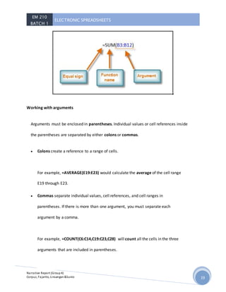
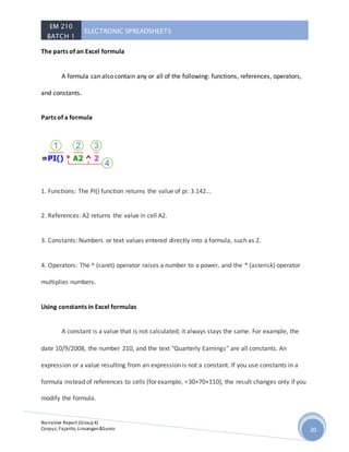
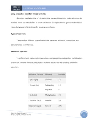
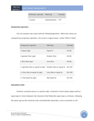
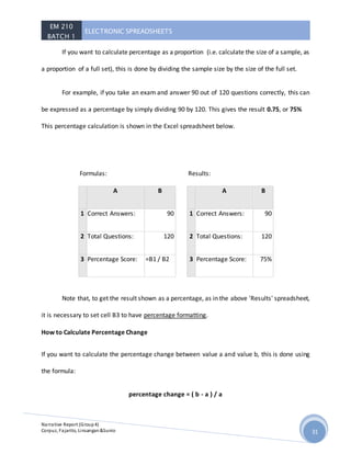
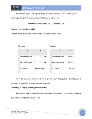
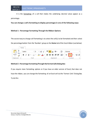
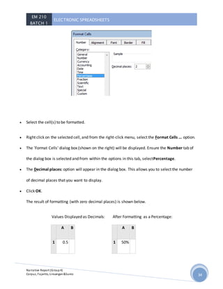
EM 210
BATCH 1
ELECTRONIC SPREADSHEETS
Narrative Report (Group4)
Corpuz, Fajarito, Linsangan&Sunio 1
Reported by: Donita Rose Linsangan (MaEd-EM)

EM 210
BATCH 1
Spread sheet
- Or worksheetisatool usedwheneveryouneedtoperformcalculations.
These calculationscaninvolve mathematical,financialorscientificdata.There are some typical
usesof spreadsheetlike the householdtaxes,gradingsystem,income taxes,inventoriesandmortgage
payments.
Two types of spreadsheets:
Manual
-creatinga worksheetonledge paperorcolumnarusinga paper,pencil,calculator,anderaser.
Electronic
-A computergeneratedspreadsheet thatmakesthe basictaskmuch easier.
Excel isbasicallyasoftware package thatallowsyouto easilyworkwithdatain a grid-like formatusing
columnsandrows to displayinformation. Being‘electronic’there are manyfeaturesthatmake iteasier
to use than the pencil andpaperversion –the mostnotable isthe abilityforourspreadsheetstobe
automaticallyrecalculatedif anyof the data inputsare laterupdated – but forthisto happenwe will
needtolearnhowto properlysetupandwrite spreadsheetformulas
Usesof an electronicspread sheet:
 cash flowanalysis
 budgets
 inventorymanagement
 financial planning

EM 210
BATCH 1
To opena spreadsheet,firstwe needtoclickthe start button.Thentry to findthe Microsoftexcel
thenclickthe button.
ElementsofElectronic Spreadsheet
1. Row and Column
It isa horizontal blockof cellsrunningacrossthe breadthof the spreadsheet. Rowsare numbered
sequentiallyfromthe top. Columnisa vertical blockcellsidentifiedbyunique alphabetical letter.
2. Worksheet
It ismade up of row,columnswhere youcanenterlabels,numbersandformulas.
It alsocontains256 columnswithalphabetheadingand65, 536 numberedrows.
3. Cell
It isa rectangle formedbythe rowsandcolumns.
You mightnotice the rectangularhighlightsthatindicatesthe locationonthe screenof the active cell.
Thiscalledthe active cell indicator (blue)
The combinationof the columnletterandthe row numberiscalledcell referencesorcell address.(Red)
4. Range
Is a blockof selectedcells.Itisalsoa selectionof multiple cells.
5. Menu Bar
The menubar displaysall of the menusavailable foruse inExcel.The contentof anymenucan be
displayedbyleftclickingthe menuname.

EM 210
BATCH 1
6. ColumnHeading,Name Box andFormulaBar
Columnheadingseachspreadsheetcontainscolumnsoeachcolumnisnamedbya letteror
combinationof letters.
Name box showsthe addressof the current selectionoractive cell.
Formulabar displaysinformationenteredorbeingenteredasyoutype inthe currentor active
cell.The contentof cell can alsobe editedin formulabar.
The centerof the Excel windowisthe worksheetandworksheetcells –withthe row numbers
displayedonthe leftandcolumnlettersabove. Justabove the columnlettersare twoboxes – the name
box whichwe will use latertogive a name to a cell or range of cells – and the formulabar. Whenyou
clickon a specificcell - the contentsof thisactive cell will be displayedinthe formulabar. If the value 5
istypedintothe cell thisvalue will appearinthe formulabar – howeverif the value 5is a resultof a
calculation – the cellstypicallydisplaysthisvalue butthe formulabarwill listthe actual formulathatwas
writtenandissavedto thiscell. Notice thatjustto the leftof the formulabaris the FX button – which
launchesthe functionwizard –as we will see later.
Justabove the name box andformulabar isthe ribbon. Whichribbonisdisplayedwill be
determinedbywhichribbontabisselected..The tabsare justabove the ribbonbuttons – seenhere is
the home ribbon. Each ribbonisfurthersubdividedintocommontool groupssuchasClipboard,Font,
Alignmentetc.

EM 210
BATCH 1
Above the ribbononthe leftisthe quickaccess toolbar – whichyoucan customize asyousee fit
– thistoolbarisalwaysvisible–so regardlessof whichribbonisdisplayedthe buttonsplacedonthe
quickaccess toolbarare alwaysone clickto use. In a similarmannerthe sizingbuttonsforthe Excel
applicationwindowandforthe spreadsheetwindow andthe helpbuttonare displayedonthe upper
righthand side.
To maneuverwithinthe spreadsheetyoucanusingthe up/downarrow keys – move yourmouse
or clickon the horizontal orvertical scroll barsat the bottomand sidesof the worksheet. Youcan also
go fromone worksheettoanotherusingthe sheettabsat the bottom. On the bottomrightof the
worksheetwindowisthe zoomtool tohelpyoueasilychange the size displayedonyourscreenw/o
impactingthe fontsize usedwithinthe spreadsheet –whichdeterminesprintsizes.

EM 210
BATCH 1

EM 210
BATCH 1
Reported by: Bryan Sunio (MaEd-EM)
Create an Excel table in a
worksheet Applies To: Excel
2013
To create a table by using the
default table style, do this:
a. Select the range of cells you want included in the table. The cells can be empty or can
contain data.
• Click Insert > Table.
• Keyboard shortcut - press Ctrl+T or Ctrl+L.

EM 210
BATCH 1
Create a table in the style you want
• Select the range of cells you want included in the table.
• On the Home tab, click Styles > Format as Table.
Set a column to a specific width
• Select the column or columns that you want to change.
• On the Home tab, in the Cells group, click Format.
• Under Cell Size, click Column Width.
• In the Column width box, type the value that you want.
• Click OK.
TIP: To quickly set the width of a single column, right-click the selected column, click Column
Width, and then type the value that you want.
Change the column width to automatically fit the contents (auto fit)
• Select the column or columns that you want to change.
• Under Cell Size, click AutoFit Column Width.
TIP: To quickly set the width of a single column, right-click the selected column, click Column
Width, and then type the value that you want.

EM 210
BATCH 1
Change the width of columns by using the mouse
Do one of the following:
• To change the width of one column, drag the boundary on the right side of the column
heading until the column is the width that you want.
• To change the width of multiple columns, select the columns that you want to change,
and then drag a boundary to the right of a selected column heading.
Set a row to a specific height
• Select the row or rows that you want to change.
• Under Cell Size, click Row Height.
• In the Row height box, type the value that you want.
Change the row height to fit the contents
• Select the row or rows that you want to change.
• Under Cell Size, click AutoFit Row Height.
• TIP: To quickly autofit all rows on the worksheet, click the Select All button, and then
double-click the boundary below one of the row headings.

EM 210
BATCH 1
Change the height of rows by using the mouse
Do one of the following:
• To change the row height of one row, drag the boundary below the row heading until
the row is the height that you want.
• To change the row height of multiple rows, select the rows that you want to change,
and then drag the boundary below one of the selected row headings.
Freeze specific rows or columns
On the worksheet, do one of the following:
• To lock rows, select the row below the row or rows that you want to keep visible when
you scroll.
• To lock columns, select the column to the right of the column or columns that you want
to keep visible when you scroll.
Before you choose to freeze rows or columns in a worksheet, it’s important to considerthe
following:
• You can freeze only rows at the top and columns on the left side of the worksheet. You
cannot freeze rows and columns in the middle of the worksheet.
• The Freeze Panes command is not available when you're in cell editing mode (that is,
you're entering a formula or data in a cell or cells) or when a worksheet is protected. To
cancel cell editing mode, press Enter or Esc.

EM 210
BATCH 1
• You can choose to freeze just the top row of your worksheet, just the left column of
your worksheet, or multiple rows and columns simultaneously. For example, if you
freeze row 1 and then decide to freeze column A, row 1 will no longer be frozen. If you
want to freeze both rows and columns, you need to freeze them at the same time.
Unfreeze rows or columns
• On the View tab, in the Window group, click the arrow below Freeze Panes.
• Click Unfreeze Panes. This unfreezes all frozen rows and columns on the worksheet.
Merge cells
Merging combines two or more cells to create a new, larger cell. This is a great way to create a
label that spans several columns. For example, here cells A1, B1, and C1 were merged to create
the label “Monthly Sales” to describe the information in rows 2 through 7.
• Select two or more adjacent cells you want to merge.
• Click Home > Merge & Center
TIP: To merge cells without centering, click the arrow next to Merge & Center, and then click
Merge Across or Merge Cells.
IMPORTANT: Make sure the data you want to end up in the merged cell is in the upper-left cell.
All data in the other merged cells will be deleted. To keep any data from the other cells, copy it
to another spot in the worksheet before you merge.

EM 210
BATCH 1
Excel keyboard shortcuts and function keys
Open a spreadsheet Ctrl+O
Go to the Home tab Alt+H
Save a spreadsheet Ctrl+S
Copy Ctrl+C
Paste Ctrl+V
Undo Ctrl+Z
Choose a fill color Alt+H, H
Cut Ctrl+X
Go to Insert tab Alt+N
Bold Ctrl+B
Center align cell contents Alt+H, A, then C
Go to Page Layout tab Alt+P
Go to Data tab Alt+A
Go to View tab Alt+W
Add borders Alt+H, B
Delete column Alt+H,D, then C
Go to Formula tab Alt+M
Function keys
F1
- Displays the Excel Help task pane.
- Ctrl+F1 displays or hides the ribbon.
- Alt+F1 creates an embedded chart of the data in the current range.
- Alt+Shift+F1 inserts a new worksheet.

EM 210
BATCH 1
F2
- Edit the active cell and put the insertion point at the end of its contents. Or, if editing is turned
off for the cell, move the insertion point into the formula bar. If editing a formula, toggle Point
mode off or on so you can use arrow keys to create a reference.
- Shift+F2 adds or edits a cell comment.
- Ctrl+F2 displays the print preview area on the Print tab in the Backstage view.
F3
- Displays the Paste Name dialog box. Available only if names have been defined in the
workbook (Formulas tab, Defined Names group, Define Name).
- Shift+F3 displays the Insert Function dialog box.
F4
- Repeats the last command or action, if possible.
- When a cell reference or range is selected in a formula, F4 cycles through all the various
combinations of absolute and relative references.
- Ctrl+F4 closes the selected workbook window.
- Alt+F4 closes Excel.

EM 210
BATCH 1
F5
- Displays the Go To dialog box.
- Ctrl+F5 restores the window size of the selected workbook window.
F6
- Switches between the worksheet, ribbon, task pane, and Zoom controls. In a worksheet that
has been split, F6 includes the split panes when switching between panes and the ribbon area.
- Shift+F6 switches between the worksheet, Zoom controls, task pane, and ribbon.
- Ctrl+F6 switches to the next workbook window when more than one workbook window is
open
F7
- Displays the Spelling dialog box to check spelling in the active worksheet or selected range.
- Ctrl+F7 performs the Move command on the workbook window when it is not maximized. Use
the arrow keys to move the window, and when finished press Enter, or Esc to cancel.
F8

EM 210
BATCH 1
- Turns extend mode on or off. In extend mode, Extended Selection appears in the status line,
and the arrow keys extend the selection.
- Shift+F8 enables you to add a nonadjacent cell or range to a selection of cells by using the
arrow keys.
- Ctrl+F8 performs the Size command (on the Control menu for the workbook window) when a
workbook is not maximized.
- Alt+F8 displays the Macro dialog box to create, run, edit, or delete a macro.
F9
- Shift+F9 calculates the active worksheet.
- Ctrl+Alt+F9 calculates all worksheets in all open workbooks, regardless of whether they have
changed since the last calculation.
- Ctrl+Alt+Shift+F9 rechecks dependent formulas, and then calculates all cells in all open
workbooks, including cells not marked as needing to be calculated.
- Ctrl+F9 minimizes a workbook window to an icon.
F10
- Turns key tips on or off. (Pressing Alt does the same thing.)
- Shift+F10 displays the shortcut menu for a selected item.
- Alt+Shift+F10 displays the menu or message for an Error Checking button.

EM 210
BATCH 1
- Ctrl+F10 maximizes or restores the selected workbook window.
F11
- Creates a chart of the data in the current range in a separate Chart sheet.
- Shift+F11 inserts a new worksheet.
- Alt+F11 opens the Microsoft Visual Basic For Applications Editor, in which you can create a
macro by using Visual Basic for Applications (VBA).
F12
- Displays the Save As dialog box.

EM 210
BATCH 1
Reported by: Ces Joanne M. Fajarito (MaEd- Math)
Basic functions

EM 210
BATCH 1
A function is a predefined formula that performs calculations using specific values in a
particular order. One of the key benefits of functions is that they can save you time
because you do not have to write the formula yourself. Excel has hundreds of functions
to assist with your calculations.
To use these functions correctly, you need to understand the differentparts of a
function and how to create arguments in functions to calculate values and cell
references.
The parts of a function
The order in which you insert a function is important. Each function has a specific
order—called syntax—which must be followed in order for the function to work
correctly. The basic syntax to create a formula with a function is to insert an equals sign
(=), function name (SUM, for example, is the function name for addition), and argument.
Arguments contain the information you want the formula to calculate, such as a range of
cell references.

EM 210
BATCH 1
Working with arguments
Arguments must be enclosed in parentheses. Individual values or cell references inside
the parentheses are separated by either colons or commas.
 Colons create a reference to a range of cells.
For example, =AVERAGE(E19:E23) would calculate the average of the cell range
E19 through E23.
 Commas separate individual values, cell references, and cell ranges in
parentheses. If there is more than one argument, you must separate each
argument by a comma.
For example, =COUNT(C6:C14,C19:C23,C28) will count all the cells in the three
arguments that are included in parentheses.

EM 210
BATCH 1
The parts of an Excel formula
A formula can also contain any or all of the following: functions, references, operators,
and constants.
Parts of a formula
1. Functions: The PI() function returns the value of pi: 3.142...
2. References: A2 returns the value in cell A2.
3. Constants: Numbers or text values entered directly into a formula, such as 2.
4. Operators: The ^ (caret) operator raises a number to a power, and the * (asterisk) operator
multiplies numbers.
Using constants in Excel formulas
A constant is a value that is not calculated; it always stays the same. For example, the
date 10/9/2008, the number 210, and the text "Quarterly Earnings" are all constants. An
expression or a value resulting from an expression is not a constant. If you use constants in a
formula instead of references to cells (for example, =30+70+110), the result changes only if you
modify the formula.

EM 210
BATCH 1
Using calculation operators in Excel formulas
Operators specify the type of calculation that you want to perform on the elements of a
formula. There is a default order in which calculations occur (this follows general mathematical
rules), but you can change this order by using parentheses.
Types of operators
There are four different types of calculation operators: arithmetic, comparison, text
concatenation, and reference.
Arithmetic operators
To perform basic mathematical operations, such as addition, subtraction, multiplication,
or division; combine numbers; and produce numeric results, use the following arithmetic
operators.
Arithmetic operator Meaning Example
+ (plus sign) Addition 3+3
– (minus sign) Subtraction
Negation
3–1
–1
* (asterisk) Multiplication 3*3
/ (forward slash) Division 3/3
% (percent sign) Percent 20%

EM 210
BATCH 1
Arithmetic operator Meaning Example
^ (caret) Exponentiation 3^2
Comparison operators
You can compare two values with the following operators. When two values are
compared by using these operators, the result is a logical value—either TRUE or FALSE.
Comparison operator Meaning Example
= (equal sign) Equal to A1=B1
> (greater than sign) Greater than A1>B1
< (less than sign) Less than A1<B1
>= (greater than or equal to sign) Greater than or equal to A1>=B1
<= (less than or equal to sign) Less than or equal to A1<=B1
<> (not equal to sign) Not equal to A1<>B1
Calculation order
Formulas calculate values in a specific order. A formula in Excel always begins with an
equal sign (=). Excel interprets the characters that follow the equal sign as a formula. Following
the equal sign are the elements to be calculated (the operands), such as constants or cell

EM 210
BATCH 1
references. These are separated by calculation operators. Excel calculates the formula from left
to right, according to a specific order for each operator in the formula.
Use of parentheses in Excel formulas
To change the order of evaluation, enclose in parentheses the part of the formula to be
calculated first. For example, the following formula produces 11 because Excel performs
multiplication before addition. The formula multiplies 2 by 3 and then adds 5 to the result.
=5+2*3
In contrast, if you use parentheses to change the syntax, Excel adds 5 and 2 together
and then multiplies the result by 3 to produce 21.
=(5+2)*3
In the following example, the parentheses that enclose the first part of the formula
force Excel to calculate B4+25 first and then divide the result by the sum of the values in cells
D5, E5, and F5.
=(B4+25)/SUM(D5:F5)
Using functions and nested functions in Excel formulas
Functions are predefined formulas that perform calculations by using specific values,
called arguments, in a particular order, or structure. Functions can be used to perform simple
or complex calculations.

EM 210
BATCH 1
Nesting Excel functions
In certain cases, you may need to use a function as one of the arguments of another
function. For example, the following formula uses a nested AVERAGE function and compares
the result with the value 50.
1. The AVERAGE and SUM functions are nested within the IF function.
Valid returns
When a nested function is used as an argument, the nested function must return the
same type of value that the argument uses. For example, if the argument returns a TRUE or
FALSE value, the nested function must return a TRUE or FALSE value. If the function doesn't,
Excel displays a #VALUE! error value.
Nesting level limits
A formula can contain up to seven levels of nested functions. When one function (we'll
call this Function B) is used as an argument in another function (we'll call this Function A),

EM 210
BATCH 1
Function B acts as a second-level function. For example, the AVERAGE function and the SUM
function are both second-level functions if they are used as arguments of the IF function. A
function nested within the nested AVERAGE function is then a third-level function, and so on.
Using references in Excel formulas
A reference identifies a cell or a range of cells on a worksheet, and tells Excel where to
look for the values or data you want to use in a formula. You can use references to use data
contained in different parts of a worksheet in one formula or use the value from one cell in
several formulas. You can also refer to cells on other sheets in the same workbook, and to other
workbooks. References to cells in other workbooks are called links or external references.
The A1 reference style
By default, Excel uses the A1 reference style, which refers to columns with letters (A
through XFD, for a total of 16,384 columns) and refers to rows with numbers (1 through
1,048,576). These letters and numbers are called row and column headings. To refer to a cell,
enter the column letter followed by the row number. For example, B2 refers to the cell at the
intersection of column B and row 2.
To refer to Use
The cell in column A and row 10 A10
The range of cells in column A and rows 10 through 20 A10:A20

EM 210
BATCH 1
To refer to Use
The range of cells in row 15 and columns B through E B15:E15
All cells in row 5 5:5
All cells in rows 5 through 10 5:10
All cells in column H H:H
All cells in columns H through J H:J
The range of cells in columns A through E and rows 10 through 20 A10:E20
Making a reference to another worksheet
In the following example, the AVERAGE function calculates the average value for the
range B1:B10 on the worksheet named Marketing in the same workbook.
Reference to a range of cells on another worksheet in the same workbook
1. Refers to the worksheet named Marketing
2. Refers to the range of cells between B1 and B10, inclusively
3. Separates the worksheet reference from the cell range reference

EM 210
BATCH 1
The difference between absolute, relative and mixed references
Relative references
A relative cell reference in a formula, such as A1, is based on the relative position of the
cell that contains the formula and the cell the reference refers to. If the position of the cell that
contains the formula changes, the reference is changed. If you copy or fill the formula across
rows or down columns, the reference automatically adjusts. By default, new formulas use
relative references. For example, if you copy or fill a relative reference in cell B2 to cell B3, it
automatically adjusts from =A1 to =A2.
Copied formula with relative reference
What occurs when you move, copy, insert, or delete worksheets
The following examples explain what happens when you move, copy, insert, or delete
worksheets that are included in a 3-D reference. The examples use the formula
=SUM(Sheet2:Sheet6!A2:A5) to add cells A2 through A5 on worksheets 2 through 6.

EM 210
BATCH 1
 Insert or copy If you insert or copy sheets between Sheet2 and Sheet6 (the endpoints in this
example), Excel includes all values in cells A2 through A5 from the added sheets in the
calculations.
 Delete If you delete sheets between Sheet2 and Sheet6, Excel removes their values from the
calculation.
 Move If you move sheets from between Sheet2 and Sheet6 to a location outside the
referenced sheet range, Excel removes their values from the calculation.
 Move an endpoint If you move Sheet2 or Sheet6 to another location in the same workbook,
Excel adjusts the calculation to accommodate the new range of sheets between them.
 Delete an endpoint If you delete Sheet2 or Sheet6, Excel adjusts the calculation to
accommodate the range of sheets between them.
Using names in Excel formulas
You can create defined names to represent cells, ranges of cells, formulas, constants, or
Excel tables. A name is a meaningful shorthand that makes it easier to understand the purpose
of a cell reference, constant, formula, or table, each of which may be difficult to comprehend at
first glance. The following information shows common examples of names and how using them
in formulas can improve clarity and make formulas easier to understand
Types of names
There are several types of names that you can create and use.

EM 210
BATCH 1
Defined name
A name that represents a cell, range of cells, formula, or constant value. You can create
your own defined name. Also, Excel sometimes creates a defined name for you, such as when
you set a print area.
Table name
A name for an Excel table, which is a collection of data about a particular subject that is
stored in records (rows) and fields (columns). Excel creates a default Excel table name of
"Table1", "Table2", and so on, each time you insert an Excel table, but you can change these
names to make them more meaningful.
For more information about Excel tables, see Using structured references with Excel tables.
Creating and entering names
You create a name by using the:
 Name box on the formula bar This is best used for creating a workbook level name for a
selected range.
 Create a name from selection You can conveniently create names from existing row and
column labels by using a selection of cells in the worksheet.

EM 210
BATCH 1
 New Name dialog box This is best used for when you want more flexibility in creating names,
such as specifying a local worksheet level scope or creating a name comment.
NOTE: By default, names use absolute cell references.
You can enter a name by:
 Typing Typing the name, for example, as an argument to a formula.
 Using Formula AutoComplete Use the Formula AutoComplete drop-down list, where valid
names are automatically listed for you.
 Selecting from the Use in Formula command Select a defined name from a list available from
the Use in Formula command in the Defined Names group on the Formula tab.
Two Percentage Calculation Types
Examples of each of these two percentage types are:
Percentage as
a Proportion
E.g. if, out of 120 questions, you answer 90 correctly, how is this
expressed as a percentage score?
Percentage
Change
E.g. if your sales figures are $1,250 in January and $1,750 in February,
what is the percentage increase in February, compared to January?
How to Calculate a Percentage as a Proportion

EM 210
BATCH 1
If you want to calculate percentage as a proportion (i.e. calculate the size of a sample, as
a proportion of a full set), this is done by dividing the sample size by the size of the full set.
For example, if you take an exam and answer 90 out of 120 questions correctly, this can
be expressed as a percentage by simply dividing 90 by 120. This gives the result 0.75, or 75%
This percentage calculation is shown in the Excel spreadsheet below.
Formulas:
A B
1 Correct Answers: 90
2 Total Questions: 120
3 Percentage Score: =B1 / B2
Results:
A B
1 Correct Answers: 90
2 Total Questions: 120
3 Percentage Score: 75%
Note that, to get the result shown as a percentage, as in the above 'Results' spreadsheet,
it is necessary to set cell B3 to have percentage formatting.
How to Calculate Percentage Change
If you want to calculate the percentage change between value a and value b, this is done using
the formula:
percentage change = ( b - a ) / a

EM 210
BATCH 1
For example if your sales figures are $1,250 in January and $1,750 in February, the
percentage change in February, compared to January, is given by:
percentage change = ( $1,750 - $1,250 ) / $1,250
This gives the result 0.4, or +40%
This percentage calculation is shown in the Excel spreadsheet below.
Formulas:
A B
1 Jan Sales Figure: $12,500
2 Feb Sales Figure: $17,500
3 % Change: =(B2 - B1) / B1
Results:
A B
1 Jan Sales Figure: $12,500
2 Feb Sales Figure: $17,500
3 % Change: 40.0%
As in the previous example, in order to get the result displayed as a percentage, it is
necessary to set cell B3 to havepercentage formatting.
Formatting to Display Percentages in Excel Cells
Percentages in Excel are stored as decimal values. For example, 25% is stored as the value
0.25, 50% is stored as the value 0.5, etc.

EM 210
BATCH 1
It is the formatting of a cell that makes the underlying decimal value appear as a
percentage.
You can change a cell's formatting to display percentages in one of the following ways:
Method 1 - Percentage Formatting Through the Ribbon Options
The easiest way to change cell formatting is to select the cell(s) to be formatted and then select
the percentage button from the 'Number' group on the Home tab of the Excelribbon (seebelow):
Method 2 - Percentage Formatting Through the Format Cells Dialog Box
If you require more formatting options or if you have an older version of Excel, that does not
have the ribbon, you can change the formatting of an Excel cell via the 'Format Cells' Dialog Box.
To do this:

EM 210
BATCH 1
 Select the cell(s) to be formatted.
 Right click on the selected cell, and from the right-click menu, select the Format Cells ... option.
 The 'Format Cells' dialog box (shown on the right) will be displayed. Ensure the Number tab of
the dialog box is selected and from within the options in this tab, selectPercentage.
 The Decimal places: option will appear in the dialog box. This allows you to select the number
of decimal places that you want to display.
 Click OK.
The result of formatting (with zero decimal places) is shown below.
Values Displayed as Decimals:
A B
1 0.5
After Formatting as a Percentage:
A B
1 50%

EM 210
BATCH 1
2 0.75 2 75%

EM 210
BATCH 1

EM 210
BATCH 1
Reported by: Ma. Cristina Corpuz (MaEd-English)
Aside from basic formulas, Microsoft Excel was also designed for various accounting
functions. Anyone who may want to start a small and simple business can use MS Excel for
maintaining accounting data such as cash transactions, book keeping or basically just a general
ledger for their business.
MS Excel comes with functionality that can perform simple to complex mathematical
calculations. It makes the business of book keeping easier since you do not have to manually
calculate transaction. Sometimes, all you have to do is create the formula needed, input the data
in the spreadsheet and you will have the result instantly.
Also, you can import or download pre-made spreadsheet templates from the Web based
on what you need and customize it your liking as well.
1. Maintaining Invoices/Budget
A simple method for you to use MS Excel is by making simple invoices and personal
budgets. An invoiceis adocument issuedby the buyer to the sellerwhich contains description
of trading parties, lists and quantifies sold items, date of payment or shipment prices,
discounts or delivery terms.
A personal budget on the other hand, is simply a plan used to decide the amount of
money that will be spent and how it will be spent.

EM 210
BATCH 1
You can use MS Excel to create invoices for your business or make your personal budget.
We can follow the steps in creating invoices and budgets:
CREATING AN INVOICE:
1. Click the Start menu and click the MS Excel icon.
2. If you want to customize your invoice, click the Page Layout to format the layout of your
spreadsheet.
3. Create the invoice heading. This must be written in a large font so when you open the
document, this is the first thing that you will and will serve as the label of the document.
Details that you may include in your heading are the following:
a. company name
b. the word “invoice” or the type of invoice you are making
c. invoice date
d. invoice number (optional)
4. After creating the heading, you may enter the recipient’s details. Make sure that the
details are complete. The details of the sender may be similar to the details you will
include for the recipient.
5. When you have inputted the sender and recipient details, you can now input billing
information such as:
a. product or service
b. quantity
c. price
d. calculated column for totaling

EM 210
BATCH 1
6. Display the amount of the total bill and terms of payment of the invoice transaction. Do
not forget to save your work to avoid losing important information.
In making a personal budget, these are the steps that you need to follow:
1. Enter the name of the budget you want to create.
2. Enter column titles in the second row. The column titles will be the categories you
want to include in your budget such as date, expense category, memo/reminder,
expense amount, income and balance.
3. Fill up the row with the expense item and enter the balance formula you need. The
formula could be as simple as the Auto Sum function, Deduction, Multiplication or
Division.
4. Continue to fill up the expense formulas until you are done with every expense that
needs to be paid.
5. Again, do not forget to click save.
VARIOUS TRANSACTIONS IN EXCEL
Aside from making invoices and budgets, you can also use MS Excel in doing the following:
 cash transactions
 accounts receivable and payable
 summaries of transactions
 book keeping
 general ledger
The calculated running total is a function which helps us keep a running total of several
items in a spreadsheet. To create the running total, follow the steps:

EM 210
BATCH 1
1. Type the information on the first row of the cells in a blank spreadsheet.
2. Input the information needed.
3. Enter the formula =SUM($letter$number:letter and number).
4. Clickon the first cellwith amount and drag the smallbox found when you highlight
a cell.
MAINTANING DAILY AND MONTHLY SALES REPORTS
In managing a business, it is possible to have lots of information that it may be difficult to
locate information. There may be daily and monthly, even yearly sales reports that you have to
sift through. Also organizing sales reports may be a bit tasking.
To help you locate information or organize data, you may use a pivot table. A pivot table
may be created sothat the categories and entries that you need willappear in anew spreadsheet.
You may also create a chart or graph for the data you have. To create a pivot table, follow the
steps:
1. Pick the spreadsheet you want to organize or analyze.
2. Go to Insert and click on the Pivot Table icon.
3. A dialog box will appear. Excel will automatically select the data for you and the pivot
table will be located in another spreadsheet.
4. The Pivot Table field appears with the different categories of the data. You have to drag
the fields that you need and a pivot table will be created for you.

EM 210
BATCH 1

Electronic Spreadshet

More Related Content

Similar to Electronic Spreadshet

More from Ces Joanne Fajarito

Recently uploaded

Electronic Spreadshet