Download to read offline

![Note that, in general, [H(t), H(t0
)] 6= 0, so we cannot write the time evolution operator in the normal way,
U(t) = exp
−i
R t
0
H(t0
) dt0
. Instead, we would have to use something called the time ordering operator, T
←
,
but even that doesn’t help us to put the evolution operator in closed form.
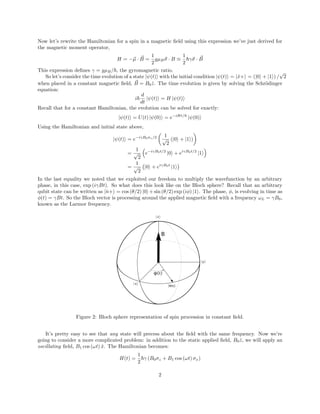
Instead we will take a different approach. What does the evolution of the state look like in a reference
frame that is rotating at the Larmor frequency? To do this, we define a new state variable in this rotating
frame, the unwound state,
|ψ0
(t)i = eiωLσzt/2
|ψ(t)i
Now does this state evolve in time?
i~
d
dt
|ψ0
(t)i = (i~)iωLσz/2 |ψ0
(t)i + eiωLσzt/2
i~
d
dt
|ψ(t)i
= −
~ωLσz
2
|ψ0
(t)i + eiωLσzt/2
H(t) |ψ(t)i
= −
~ωLσz
2
|ψ0
(t)i + eiωLσzt/2
H(t)e−iωLσzt/2
eiωLσzt/2
|ψ(t)i
=
−
~ωLσz
2
+ eiωLt/2
H(t)e−iωLσzt/2
|ψ0
(t)i
= H0
(t) |ψ0
(t)i
Which defines the Hamiltonian in the rotating frame:
H0
(t) =
−
~ωL
2
σz + eiωLσzt/2
H(t)e−iωLσzt/2
We’ll focus on this last term:
eiωLσzt/2
H(t)e−iωLσzt/2
=
~γ
2
eiωLσzt/2
(B0σz + B1 cos (ωt) σx) e−iωLσzt/2
=
~γ
2
B0σz + eiωLσzt/2
B1 cos(ωt)σxe−iωLσzt/2
Let’s rewrite the field as two counter rotating circular waves:
cos(ωt)σx =
1
2
((cos(ωt)σx + sin(ωt)σy) + (cos(ωt)σx − sin(ωt)σy))
= e−iωt
σ+ + eiωt
σ−
+ eiωt
σ+ + e−iωt
σ−
Here we have used the raising and lowering Pauli operators, σ± = (σx ± iσy) /2. Now we need to calculate
the transformation, exp(iασz)σ± exp (−iασz):
eiασz
σ+e−iασz
=
eiα
0
0 e−iα
0 1
0 0
e−iα
0
0 eiα
=
0 e2iα
0 0
= e2iα
σ+
eiασz
σ+e−iασz
=
eiα
0
0 e−iα
0 0
1 0
e−iα
0
0 eiα
=
0 0
e−2iα
0
= e−2iα
σ−
So,
H0
(t) = −
~ωL
2
σz +
~γ
2
B0σz + B1eiωLσzt/2
cos (ωt) σxe−iωLσzt/2
= −
~ωL
2
σz +
~ωL
2
σz +
~γ
2
B1eiωLσzt/2
e−iωt
σ+ + eiωt
σ−
+ eiωt
σ+ + e−iωt
σ−
e−iωLσzt/2
=
~γ
2
B1
ei(ωL−ω)t
σ+ + ei(ω−ωL)t
σ−
+
ei(ω+ωL)t
σ+ + e−i(ω+ωL)t
σ−
3](https://image.slidesharecdn.com/electronspinresonance-210425174606/85/Electron-spin-resonance-3-320.jpg)

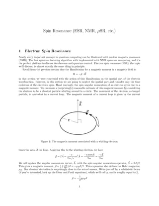
This document discusses electron spin resonance (ESR), which is similar in principle to nuclear magnetic resonance (NMR). It derives the magnetic moment of an electron's spin and shows that a spin placed in a constant magnetic field will precess around the field at the Larmor frequency. When an additional oscillating magnetic field is applied at the Larmor frequency, the spin will rotate at the Rabi frequency in the rotating frame. This rotation appears as oscillations between the spin states on the Bloch sphere in the lab frame.