Download to read offline
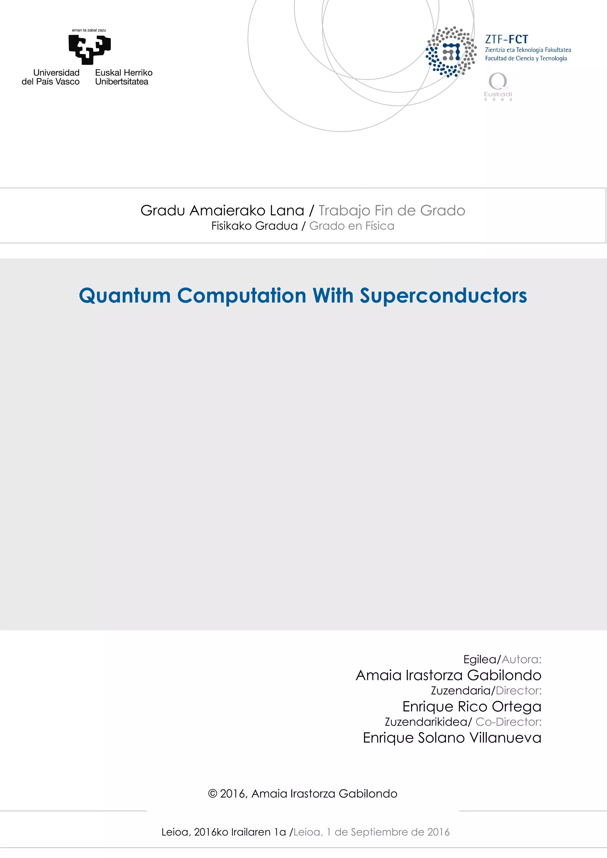

![1 General description of a qubit
The qubit (quantum bit) is the fundamental element of quantum information and quantum
computation, analogous to the classical bit. The same way the classical bit can be in two
states, 0 and 1, the qubit can also be in two possible states |0i and |1i which are the
computational basis states. The difference is that the qubit can be in a superposition of
its basis states, which is a fundamental property of quantum computing. Its state can be
written as a linear combination of the basis states
|ψi = α |0i + β |1i (1)
When we measure the state of the qubit there is a |α|2 probability of measuring |0i and
|β|2 probability of measuring |1i, being |α|2 + |β|2 = 1. We can also write α and β like
α = cos
θ
2
(2)
and
β = eiϕ
sin
θ
2
(3)
where the angles θ and ϕ define the Bloch sphere. Classical bits can only be in the north
or south poles of the sphere, while a qubit can be in any point of the sphere.
Figure 1: Graphical representation of a qubit using the Bloch sphere. Besides the classically
possible states |0i and |0i superposed |Ψi states are also possible.
Measurements change the state of the qubit, this being a fundamental postulate of
quantum mechanics. Thus, when we make a measurement in a qubit and it gives |1i it will
change its state to |1i.
Even if a qubit can be in a superposition of its basis states, a single measurement can
only give us one bit of information, either |0i or |1i[1].
4](https://image.slidesharecdn.com/quantumcomputationwithsuperconductors-210425174826/75/Quantum-computation-with-superconductors-5-2048.jpg)
![2 Quantum computation and quantum information
A quantum computation is a physical process based in the laws of quantum mechanics
where an input state is transformed in an output state of a system. The input and output
states are given by the quantum states of the system. Quantum computation is performed
by qubits, which are the system that gives us the input and output and where operations are
performed. Qubits can encode any number of inputs and outputs using the binary notation
and quantum entanglement between qubits. That is, the base of quantum computation
are quantum superposition and quantum entanglement[2]. The mentioned operations are
performed by quantum gates, which are quantum processes that transform qubit states.
Quantum computation is thought to give many advantages comparing to classical com-
puting, as the laws of quantum mechanics give the ability to do more than just with the
laws of classical mechanics. Quantum computers are thought to be able to solve problems
that classical computers cannot solve, as it is thought to be exponentially faster and takes
less resources. This is based in the idea of quantum parallelism. In a classical computer
we perform an operation in a bit 0 and another in a bit 1. In a quantum computer just
one operation would be needed, because a qubit is in a superposition of both states |0i
and |1i. This way we perform the same operation using just one qubit instead of the two
classical qubits. More formally, in a classical computer one must run it n times to compute
a function f : N → N for the numbers 1, 2, .., n. With a quantum computer it is possible
to do the same by
|1i |0i → |1i |f(1)i (4)
|2i |0i → |2i |f(2)i (5)
...
|ni |0i → |ni |f(n)i (6)
But, we can also prepare the following input state, being a quantum superposition of the
previous states
|ψi =
1
√
n
n
X
k=1
|ki |0i (7)
Running this state just once in a quantum computer we obtain the state
1
√
n
n
X
k=1
|ki |f(k)i (8)
Thus, we get all the values of f in a quantum superposition by running the quantum com-
puter just once. The problem is that it is not possible to read out all of the states in a
measurement, it is only possible to read out certain information.[1][3]
5](https://image.slidesharecdn.com/quantumcomputationwithsuperconductors-210425174826/75/Quantum-computation-with-superconductors-6-2048.jpg)
![The purpose of quantum computers is the management of quantum information, the
information encoded in qubits. They are thought to be able to solve algorithms that are
impossible for classical computers. They should solve problems that need a huge amount of
operations, that classical computers would need a impossible amount of time and resources
to solve. Another advantage is that they would be able to simulate quantum phenomena
that is impossible to simulate using classical computers.
The study of the manipulation of this quantum information is referred to as quantum
information science (QIS). The first definition of QIS was given in a workshop with the
same name by the National Science Foundation of the United States in 1991[4]:
Quantum information science (QIS) is a new field of science and technology, combin-
ing and drawing out disciplines of physical science, mathematics, computer science, and
engineering. Its aim is to understand how certain fundamental laws of physics discov-
ered earlier in this century [20th] can be harnessed to dramatically improve the acquisition,
transmission, and processing of information.
Quantum information science has had many successes, not necessarily related to the
construction of quantum computers. It has shown that quantum mechanics is more than
what it was thought when it was first studied. It has proved to be a theory of transmission
of information in addition to just a theory of matter and energy as it was first thought. Also,
it has brought discussions of what we understand as the quantum world. Finally, it has
defined a set of experimentally used metrics, such as fidelity or decoherence time, making
possible discussion and comparison of quantum system that was previously impossible.
6](https://image.slidesharecdn.com/quantumcomputationwithsuperconductors-210425174826/75/Quantum-computation-with-superconductors-7-2048.jpg)
![When we talk about the causes of decoherence, the decohering elements can be extrinsic
and intrinsic. The extrinsic decoherence is caused the already mentioned coupling to the
environment, and the solution will be isolating our system as much as possible (as it must be
still readable). Intrinsic decoherence is caused by noise coming from the superconducting
circuit. Given the importance of this noise it will be better explained later.
4.2.1 Decoherence rates
Long enough coherence times are essential for quantum computing, the qubit must remain
long enough in a coherent state so that measurement and implementation of qubit gates
is possible. Qubits are characterized by two times, T1 and T2. T1 is the time required by
a qubit to relax from the first excited state to the ground state[5], that is, the decay time,
which can be referred to as dissipation[6] or relaxation. T2 is the average time in which
the energy-level splitting remains unchanged or the time it takes for the phase difference
between two eigenstates to become random[5], the dephasing time[6]. It is necessary to
specify the type of experiment used to measure T2, as the dephasing time is not a unique
phase coherence time[7]. Both relaxation and dephasing arise from the weak coupling to
quantum noise in the environment. The relaxation rate comes from the fluctuations at the
frequency of the energy-level splitting. It can be written as the sum of the transition rates
from one eigenstate to the other[7]
1
T1
= Γ↑ + Γ↓ (10)
The dephasing rate has two contributions
1
T2
=
1
2T1
+
1
τΦ
(11)
The first contribution comes from the relaxation process, it represents the destruction
of the coherent superposition when the qubit transitions from one eigenstate to the other[7],
as we have introduced in (9). The difference is that, as we will explain later, the temper-
ature in which the qubits will perform will be of the order of millikelvin, meaning that
the temperature will not be a cause of decoherence. Still, (9) is the basis that illustrates
our further understanding of quantum decoherence. Decoherence will come from the noise
that will be introduced in the next chapter. The second contribution is given by the ’pure
dephasing’ τΦ, and comes from low-frequency fluctuations with exchange of infinitesimal
energy[5].
We can also define the coherence quality factor Q = πT2ω0, the number of one-qubit oper-
ations achievable before the system loses coherence[8].
Experimentally, the longest coherence times achieved for the simplest qubits before
2008 can be seen in Table.1 [5]. The coherence quality factor, on the other hand, is about
105[8].
10](https://image.slidesharecdn.com/quantumcomputationwithsuperconductors-210425174826/75/Quantum-computation-with-superconductors-11-2048.jpg)
![Qubit T1(µs) T2(µs)
Charge 2.0 2.0
Flux 4.6 1.2
Phase 0.5 0.3
Table 1: [5]Longest reported values of T1 and T2 until 2008
Figure 2: [9]This graph shows the improvement made in decoherence rates in the last years.
4.3 Noise
We have already mentioned that the loss of coherence does not come from temperature, as
it is negligible. Instead, the phenomenology above described occurs due to microscopic low-
frequency noise, also called 1/f. Introducing it briefly, 1/f noise comes from low-frequency
fluctuations. The origin of 1/f noise in superconducting qubits is not yet clear and it is
a subject of study, it is one of the physical questions that has arisen from the study of
superconducting quantum computation.
Even if the origin of 1/f noise in superconducting qubits is not completely clear, edu-
cated guesses have been made based on phenomenological models[8]. There are thought
to be three sources of 1/f noise in superconducting circuits[5]. The first is critical current
fluctuations, caused by the trapping and untrapping of electrons in defects of the tunnel
barrier. A trapped charge locally modifies the height of the tunnel barrier changing the
critical current of the junction[10]. This noise affects all superconducting qubits. The slow
fluctuations modify the energy level splitting and thus each measurement gives a slightly
different measurement. The resultant phase errors lead to decoherence.
The second source are charge fluctuations. This noise is produced by electrons jumping
11](https://image.slidesharecdn.com/quantumcomputationwithsuperconductors-210425174826/75/Quantum-computation-with-superconductors-12-2048.jpg)
![from one trap to other in the surface of the superconductor. This induces charges in nearby
superconductors. This decoherence mechanism affects charge qubits particularly, but in
the degeneracy point. With the increase of the EC/EJ value the charge qubit becomes less
susceptible to this noise.
The third source is magnetic-flux fluctuations. It is thought it arises from spin diffusion1
on the superconductor surface generated by the exchange mediated by the conduction
electrons[11]. This decoherence mechanism affects flux qubits, except in the degeneracy
point.
Low-frequency noise only affects decoherence or dephasing, it does not affect relaxation
because relaxation requires energy exchange with the environment, and 1/f noise is an
intrinsic feature of the circuit. Noise can be reduced improving the quality of the materials
used in junctions and capacitors and thus reducing the number of defects that are the cause
of noise.
Dephasing times for the CPB, for example, are of the order of nanoseconds[12]. To
enhance dephasing times two strategies can be followed. First, materials and properties of
the junction can be improved in order to eliminate intrinsic 1/f noise. Secondly, qubits can
be operated at their optimum working points and thus eliminate linear noise sensitivity. A
combination of both may be necessary in the future to build scalable quantum computers[5]
1
continuous exchange of energy between individual nuclear spins
12](https://image.slidesharecdn.com/quantumcomputationwithsuperconductors-210425174826/75/Quantum-computation-with-superconductors-13-2048.jpg)
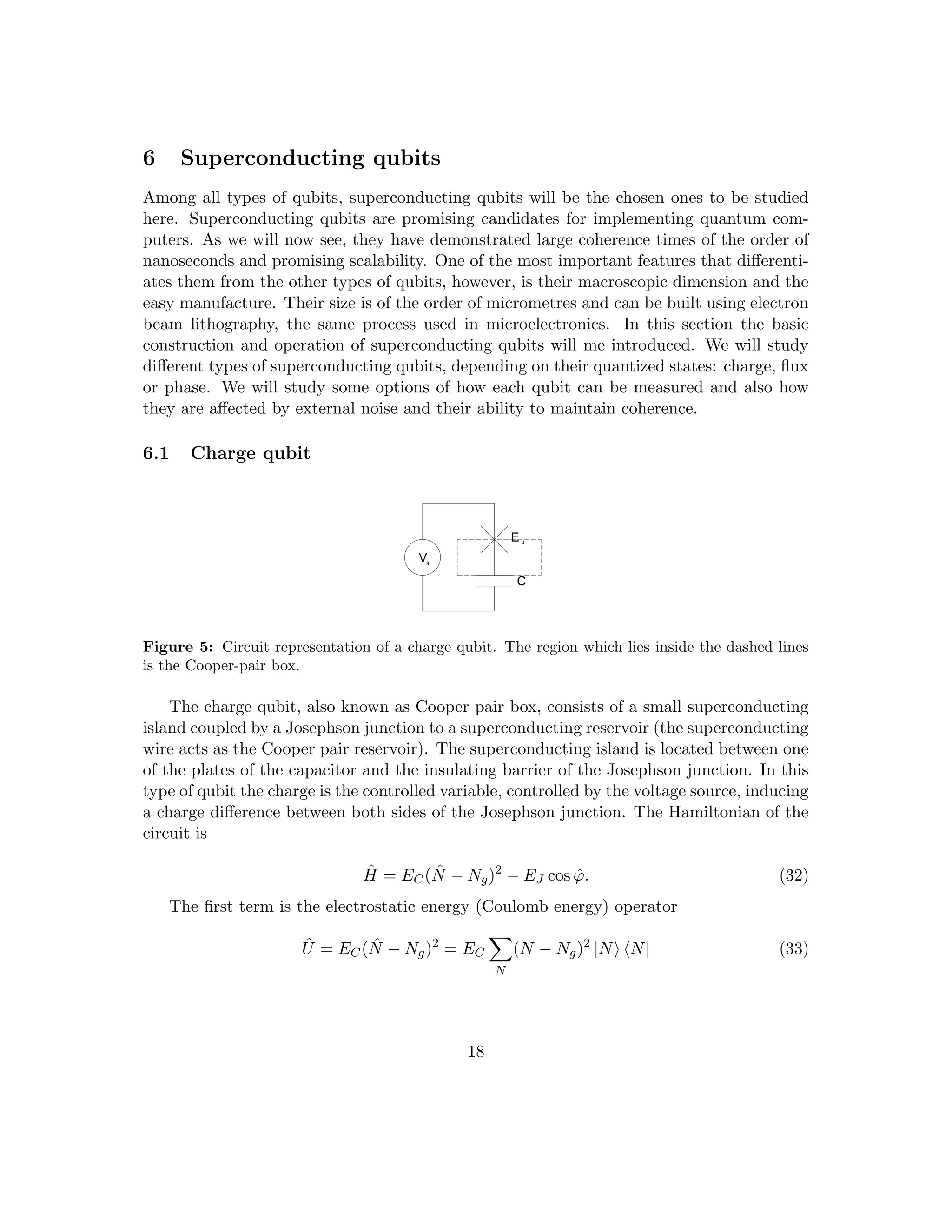
![5 Superconducting circuits
Superconducting circuits are the basis of superconducting qubits, as they are built using
superconducting elements. It is advisable to first check the basic theory of superconducting
circuits before scaling up to superconducting qubits. Our purpose for now is to study
simple superconducting circuits that behave quantum mechanically. For a circuit to behave
quantum mechanically there must be no dissipation, that is, the circuit must have zero
resistance at the (qubit) operating temperature. This is essential to preserve quantum
coherence. Non-linearity is also essential, because we want to approximate our system to
a two level qubit, meaning that the energy level cannot be uniformly spaced. The only
element which is both non-dissipative and non-linear is a Josephson junction. This makes
Josephson junctions the essential element of superconducting qubits.
5.1 Quantum LC oscillator
Figure 3: The LC circuit is the simplest possible quantum circuit, consisting of an inductor
connected to a capacitor using superconducting wire.
The first quantum circuit we will introduce is the LC oscillator, as it is the simplest
example of a quantum integrated circuit. Studying the simplest case will help us understand
the circuits of the superconducting qubits and their Hamiltonians. LC circuits consist
of an inductor L connected to a capacitor C. All of the wires connecting the elements
must be superconducting for the circuit to be quantum, this way the energy levels in the
superconducting gap will be discrete. The LC circuit obeys the equations of motion of
the linear harmonic oscillator. The flux in the inductor Φ is analogous to the position
coordinate and the charge Q on the capacitor is analogous to the conjugate momentum.
The Φ̂ and Q̂ variables are conjugate quantum operators, which do not commute [Φ̂, Q̂] = i~
[13]. Even if the circuit has a huge amount of electrons, the degrees of freedom have
been reduced to one, the Cooper-pair fluid moving back and forth in the circuit[7]. The
Hamiltonian of the circuit is
Ĥ =
Φ̂2
2L
+
Q̂2
2C
(12)
The inductance L of the system can be thought as the ’mass’ and the inverse of de
13](https://image.slidesharecdn.com/quantumcomputationwithsuperconductors-210425174826/75/Quantum-computation-with-superconductors-14-2048.jpg)
![capacitance 1/C as the ’spring constant’. Knowing the LC oscillator is analogous to the
harmonic oscillator we can write the Hamiltonian in terms of the raising and lowering
operators ω = 1/
√
LC being the resonance frequency of the circuit
Ĥ =
1
2
~ω
n
â†
â + ââ†
o
(13)
Using the commutation relation [â, â†] = 1 we can rewrite de Hamiltonian as
Ĥ = ~ω
â†
â +
1
2
(14)
where the raising and lowering operators are, consecutively
â†
= −i
1
√
2C~ω
Q̂ +
1
√
2L~ω
Φ̂ (15)
â = i
1
√
2C~ω
Q̂ +
1
√
2L~ω
Φ̂ (16)
Solving the Hamiltonian of the LC circuit (14) the difference between two consecutive
energy levels is always ∆E = ~ω, same as in the the linear harmonic oscillator. This
means that the energy levels of the LC circuit are regularly spaced and it is impossible to
approximate it to a two level system using the lowest two levels. That is why we can not use
LC circuits as qubits, even if they are able to preserve coherence due to superconductivity,
as they do not satisfy both conditions we have established before. This means that we must
introduce non-linear elements such as Josephson junctions in the circuit. Nevertheless, the
Hamiltonian of the LC circuit gives us the basis to construct the Hamiltonians of the
superconducting qubits that will be later introduced.
5.2 Superconductivity
To understand the Josephson effect, it is advisable to first acquire some notion about the
origin of superconductivity. Macroscopically, superconductivity manifests itself as a lack of
resistance, so that the current flows with no obstacles. Microscopically, it is the condensa-
tion of paired electrons(Cooper pairs) into a Bose-Einstein condensate, a boson-like state.
This is caused by an attractive potential. An electron moving through a conductor attracts
positive charges in the lattice. For this reason, the lattice suffers a deformation, attracting
another electron with opposite spin due to the newly created high positive charge density
region. Thus, the electrons become correlated forming a Cooper pair. This pairing causes a
excitation gap. The pairs energy must be higher than the gap before separating into quasi-
particles again. Above the gap quasiparticle states form a continuum. The single particle
spacing will be only noticeable when the electrode is very small, of the order of nanometres.
14](https://image.slidesharecdn.com/quantumcomputationwithsuperconductors-210425174826/75/Quantum-computation-with-superconductors-15-2048.jpg)
![Superconductivity reduces a huge Hilbert space to a single quantum state |Ni, the
number of pairs moving. This state can be described by a many-body wave function where
all pairs have the same phase and energy
Ψ(~
r, t) = Ψ0(~
r, t)eiθ(~
r,t)
(17)
5.3 Josephson junctions
LJ
C C
IC
Figure 4: Circuit representation of a Josephson junction. There are many ways to represent
a Josephson junction using circuits. The one of the left is the one adopted generally as it is a
simplification of the others.
Josephson junctions are the essential element of superconducting qubits, as they intro-
duce the needed non-linearity to the system. They consist of two superconductor separated
by an insulating barrier. The dimension of the barrier is of the order of nanometres[5]. The
origin of the non-linearity of the Josephson element is associated with the discreteness of
charge that tunnels across the thin insulating barrier. Hence the junction is characterized
by only one degree of freedom N(t), the number of Cooper pairs having tunnelled across
the barrier. The charge that has flown across the element is QJ (t) = −2eN(t). In the
junction, the charge Q(t) in the capacitance does not need to equal QJ (t) when the junc-
tion is connected to an electrical circuit. The Josephson element can also be described by
the flux ΦJ
ΦJ =
Z t
−∞
v(t0
) dt0
(18)
where v is the voltage across the element. The current through the inductor is propor-
tional to the branch flux
15](https://image.slidesharecdn.com/quantumcomputationwithsuperconductors-210425174826/75/Quantum-computation-with-superconductors-16-2048.jpg)
![I(t) =
1
L
Φ(t) (19)
For the Josephson element this relationship can be written as[13]
I(t) = I0sin
2e
~
ΦJ (t)
= I0sin
2π
ΦJ (t)
Φ0
(20)
where I0 is the critical current through the element and Φ0 = h
2e is the superconducting
flux quantum with value Φ0 = 2.07x10⁻¹⁵Wb . The discreteness of Cooper pairs tunnelling
through the barrier causes a periodic flux dependence of the current, with a period given by
the superconducting flux quantum Φ0. δ = 2πΦJ (t)
Φ0
is the gauge-invariant phase-difference
or simply the phase. This variable is just the electromagnetic flux in dimensionless units.
The real phase difference between the two superconducting electrodes is given by
ϕ = δmod2π (21)
It denotes the phase difference between the wave functions ψR and ψL, which describe
the Cooper pairs residing in the right and left superconductors of the junction.
The Josephson element can also be described by two other parameters. The first is the
Josephson effective inductance LJ0 = Φ0
2πI0
. Thus the Josephson phase dependent induc-
tance is
LJ (δ) =
∂I
∂Φ
−1
=
LJ0
cos δ
(22)
The second parameter is the Josephson energy
EJ =
Φ0
2π
I0 (23)
the required energy to store a Φ0 flux quantity in the Josephson inductor. If we calculate
the energy stored in the junction we get
E(t) = −EJ cos
2π
Φ(t)
Φ0
(24)
The variable that gives the number of Cooper-pairs across the junction N should be
treated as a discrete operator, as we have said that the charge tunnelling across the barrier
is discrete
N̂ =
X
N
N |Ni hN| (25)
The two superconducting electrodes form a capacitor, but we will ignore the Coulomb
energy that builds up as Cooper pairs tunnel from one side to the other. The tunnelling of
16](https://image.slidesharecdn.com/quantumcomputationwithsuperconductors-210425174826/75/Quantum-computation-with-superconductors-17-2048.jpg)
![electrons through the barrier couples the |Ni states. The coupling energy is given by the
Hamiltonian
ĤJ = −
EJ
2
X
N
|Ni hN + 1| + |N + 1i hN| (26)
The Hamiltonian can be written in terms of the phase difference across the junction.
We introduce new basis states
|ϕi =
X
N
eiNϕ
|Ni (27)
Where ϕ → ϕ+2π leaves the |ϕi unaffected. ϕ̂ and N̂ operators are conjugate variables,
with uncertainty relation ∆N̂∆ϕ̂ ≥ 1 and
h
ϕ̂, N̂
i
= i. The gauge invariant phase difference
is analogous to the position operator, and N̂ = −i ∂
∂ϕ is analogous to the momentum
operator. Conversely, the |Ni state is given by the Fourier transformation of the phase
state
|Ni =
1
2π
Z 2π
0
dϕeiNϕ
|ϕi (28)
We introduce the operator
eiϕ̂
=
1
2π
Z 2π
0
dϕeiϕ
|ϕi hϕ| (29)
Which acts in |Ni as
eiϕ̂
|Ni = |N − 1i (30)
We can obtain the expression for the coupling Hamiltonian (26) in this new basis as[14]
ĤJ = −
EJ
2
(eiϕ̂
+ e−iϕ̂
) = −EJ cos ϕ̂ (31)
We see that equation (31) is the quantum equivalent of equation (24). More correctly, if
we solve the Hamiltonian in the right ϕ̂ basis, the eigenvalues we get are given by equation
(24).
17](https://image.slidesharecdn.com/quantumcomputationwithsuperconductors-210425174826/75/Quantum-computation-with-superconductors-18-2048.jpg)
![where Ng = Cg
Vg
2e is the dimensionless gate charge or offset charge, the polarization
charge induced by the voltage on the gate capacitor. EC = (2e)2
2(CJ +Cg) is the electrostatic
Coulomb energy, the energy used to store a Cooper pair in the capacitor. The second term
belongs to the Josephson coupling energy (31) introduced before. The charge qubit is in
the charge regime, EC EJ , which means that the variable N̂ is well defined and the
phase ϕ̂ fluctuates. N̂ is a discreet variable representing the quantity of Cooper pairs on
the island which can only take integer values. The offset charge Ng is, on the other side, a
continuous variable.
The charge states are given by the excess of Cooper pairs that have tunnelled to the
island. For a qubit, all the states over |2i can be ignored when the offset charge is about
the same charge as an electron, Ng = 1/2, because of a great energy difference between
the first and second states. Thus, we can make a two level approximation.
The qubit basis states are |0i and |1i, the first corresponding to the lack of Cooper
pairs in the superconducting island and the second corresponding to the presence of a
single Cooper pair. When Ng = 1/2, the energy is the same for both charge states |0i and
|1i leading to degeneracy. For that reason an energy splitting occurs in that region and
the energy eigenstates become linear combinations of the charge states. At the degeneracy
point the energy eigenstates are |gi = 1/
√
2(|0i + |1i) and |ei = 1/
√
2(|0i − |1i)2. The
energy splitting in this point is ∆, but we can write the general energy splitting as
∆E =
p
∆2 + ε2 (34)
where ε = EC(Ng − 1/2).
Making the two level approximation, we can write the qubit reduced Hamiltonian as[15]
Ĥqubit = EC
N2
g 0
0 (1 − Ng)2
−
EJ
2
0 1
1 0
(35)
If we change the zero of energy of the system to E0 = EC(1/2 − Ng)2 we can rewrite
the reduced Hamiltonian as
Ĥqubit = ECσ̂Z −
EJ
2
σ̂X (36)
The eigenvalues and eigenstates of the Hamiltonian are solutions to the Mathieu equa-
tion. The level of anharmonicity of the system depends on the relation EJ /EC. When it
gets higher, the qubit spectrum becomes more and more uniformly spaced and the system
starts behaving like a linear harmonic oscillator.
2
g stands for ground state and e stands for first excited state
19](https://image.slidesharecdn.com/quantumcomputationwithsuperconductors-210425174826/75/Quantum-computation-with-superconductors-20-2048.jpg)
![Charge dispersion determines the variation of energy levels. It differs depending on the
environment offset charge and the gate voltage, and determines the sensitivity of the CPB
to charge noise. The dispersion can be defined as[16]
m = Em(Ng = 1/2) − Em(Ng = 0) (37)
Where Em are the energy eigenvalues. The smaller the charge dispersion, the less the
qubit frequency will change in response to gate charge fluctuations. The charge dispersion
decreases rapidly with EJ /EC. When the CPB works in the flux regime with EJ EC,
the decrease of charge dispersion and the uniformity of the qubit spectrum influence the
operation of the system as a qubit.
To read-out the state of the CPB qubit a single-electron transistor (SET) is used. The
SET is a sensitive electrometer. It consists of a superconducting island connected by two
Josephson junctions. When the voltages across the junctions are near the degeneracy point
Ng = 1/2, charges cross the junctions inducing a current flow through the SET. If we cou-
ple the CPB island to the SET island using a capacitance, a contribution to the SET
voltage is made and thus the SET current depends on the CPB state. When the Josephson
junctions are small the phase coherence is destroyed by environmental fluctuations, that
is, the current flow is dissipative. For this reason the read-out is made by measuring the
resistance of the SET.
As it has been said before, the CPB is sensitive to low-frequency noise, which reduces
its coherence times. To reduce this problem, other qubits based on the CPB have been
designed, such as the quantronium and the transmon.
6.1.1 Quantronium
Vg
EJ detector
C
Figure 6: Circuit representation of a quantronium qubit.
The quantronium qubit consists of two Josephson junctions and a capacitance Cg sepa-
20](https://image.slidesharecdn.com/quantumcomputationwithsuperconductors-210425174826/75/Quantum-computation-with-superconductors-21-2048.jpg)
![rated by a superconducting island. The two Josephson junctions are connected to a bigger
one with a higher critical current, forming a closed superconducting circuit. The big junc-
tion is used to measure the state of the qubit. A external flux Φe is applied through the
loop. The quantronium was the first qubit to use the charge degeneracy point to mitigate
low-frequency noise and thus extend dephasing times. Since it is a closed circuit with
applied external flux, this is a new noise channel that should be operated at the flux de-
generacy point.
In the double degeneracy point3 the qubit is insensitive to low-frequency (1/f) charge
and flux noise. Linear noise is not able to change the qubit transition frequency, because
the eigenenergies have no slope in the degeneracy point. This point is called the optimum
working point. Success of the optimum working point has been shown experimentally [5].
The insensitivity to both charge and flux means that the two qubit states can not be dis-
tinguished at the degeneracy point.
To measure the qubit state a current pulse is applied moving the qubit away from the
flux degeneracy point. This pulse produces a clockwise or anticlockwise current in the
loop, depending on the qubit state. The direction of the current is detected by the third
junction. The new current adds or subtracts from the induced current pulse. This affects
the read-out junctions bias-current making it higher or lower. Thus, the junction switches
out of the zero-voltage state. Measuring the voltage and seeing if it positive or negative
we can determine the state of the qubit.
With quantronium qubits much longer relaxation and decoherence times are obtained
comparing to a Cooper-pair box. Saclay group extended the dephasing time T2∗ about
three orders of magnitude (∼ 500ns)[17].
6.1.2 Transmon
The transmon consists of two superconducting islands coupled through two Josephson junc-
tions. It is basically a CPB, only that it is operated in the flux regime EJ EC, normally
EJ /EC ∼ 50. This increases dephasing times in various orders, as much as three orders of
magnitude (from nanoseconds to microseconds) [18].The Cooper pair box is sensitive to 1/f
charge noise even in the degeneracy point, when its affected by external charge fluctuators.
Operating the transmon at the flux regime solves this problem.
The Hamiltonian of the transmon is the same as in the CPB (32), considering that
both junctions are identical, with the difference that we have an additional capacitance,
meaning that EC = (2e)2/(CJ + CB + Cg).
3
That is Ng = 1/2 and Φe = mΦ0/2, where m is an integer.
21](https://image.slidesharecdn.com/quantumcomputationwithsuperconductors-210425174826/75/Quantum-computation-with-superconductors-22-2048.jpg)
![C g
C B
Figure 7: Circuit representation of a transmon qubit. The region which lies inside the dashed
lines is the Cooper-pair box.
As EJ /EC increases, the eingenenergies flatten, meaning that every point can be
considered an optimum operating point. Charge dispersion decreases exponentially with
p
EJ /EC, the dispersion being m ∝ e−
√
8EJ /EC , as the anharmonicity decreases slower.
Thus, the qubit transition frequency is very stable respect to charge noise. As the qubit
is immune to charge noise, coherent control is possible and dephasing times T∗
2 ∼ 2µs
approaching T∗
2 = 2T1 are possible. In the large EJ /EC limit, the charge fluctuations are
given by[18]
∆N̂ =
q
N̂2 m − N̂ 2
m ' (m + 1/2)1/2
EJ
8EC
1/4
(38)
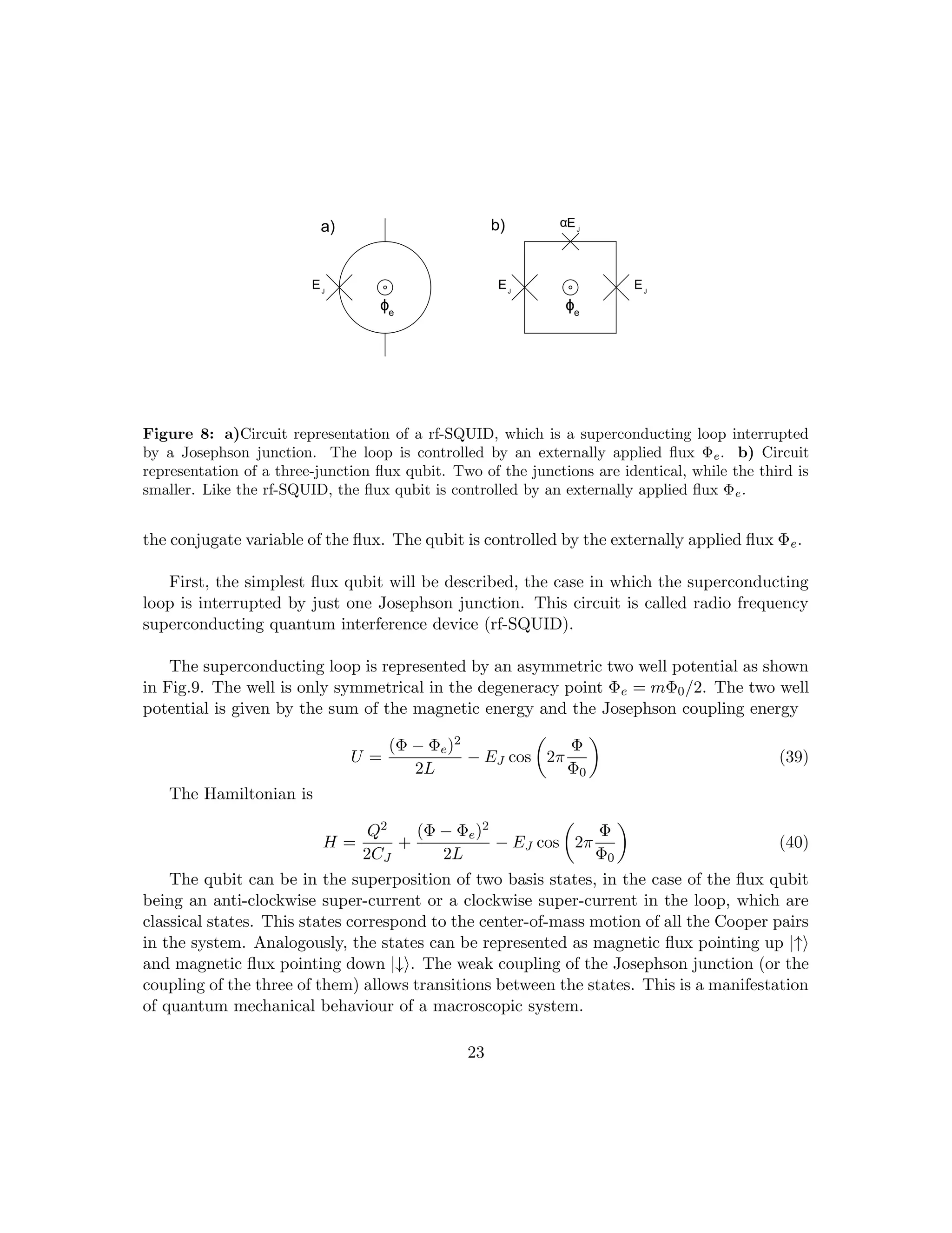
6.2 Flux qubit
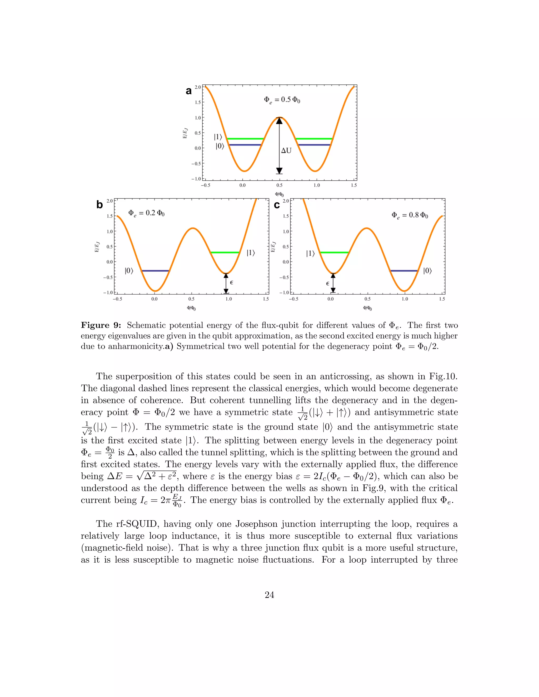
The flux qubit is constituted by a superconducting loop of inductance L interrupted by one
(rf-SQUID) or three Josephson junctions. When a weak magnetic field is applied through
the superconducting loop, a current is induced. This happens even if there is a Josephson
junction interrupting the superconducting loop.
Like it might be guessed from its name, flux qubits work in the flux regime, that is,
EJ EC, more accurately, EJ /EC ∼ 50, where the phase degree of freedom becomes
dominant, which means that in this case the phase is the discrete variable. Even if it works
in the same regime as the transmon qubit, the flux qubit is completely different while both
the superconducting circuit and the discrete variable are different. The macroscopic de-
gree of freedom is the flux Φ induced in the loop, that is, the integral of the voltage across
the inductance L (18). The flux, like the charge in the charge qubit, is quantized. The
quanta is called the fluxon and quantization comes from the relation between the phase
and the total flux (Φ0/2π)ϕ + Φe + Φ = mΦ0, where m is an integer. The continuous vari-
able is the charge Q on the capacitance CJ , which in this case is the continuous variable,
22](https://image.slidesharecdn.com/quantumcomputationwithsuperconductors-210425174826/75/Quantum-computation-with-superconductors-23-2048.jpg)
![critical current Ic(Φe) which depends on the dc-SQUID inductance LJ .
6.2.1 Fluxonium
Cg
g
C
g
C
g
C
g
C
Figure 11: Circuit representation of the fluxonium qubit. The loop is formed by a small Josephson
junction shunted by the an array of junction of bigger area. The islands formed between the larger
junctions are connected to ground by capacitances Cg.
The fluxonium qubit is based on superinductance. Superinductance has two essential
properties: it must superconduct direct current (DC) and it must present the impedance of
a frequency independent inductance L to an alternating current (AC).The impedance must
have a stray capacitance Cs small enough so that
p
L/Cs RQ where RQ = h/(2e)2 '
6.5kΩ is the superconducting impedance quantum.
The fluxonium qubit consists of a small Josephson junction shunted by an array of
larger area junctions. A simple way to understand it is to think of it as a superconducting
loop interrupted by N + 1 Josephson junctions, one of them being weaker than the rest,
called the black-sheep junction. As in the flux qubit, the quantum states are given by the
fluxons, the flux quanta trapped in the loop. Fluxons can escape the loop across one of
the junctions by a phase-slip. The junction array stores the inductive energy associated
with the phase-slip, the energy needed to charge the loop with a fluxon. The black-sheep
junction allows the fluxon number to change coherently by a unity[19].
The Hamiltonian is given by
Ĥ = ECN̂2
+
1
2
ELϕ̂2
− EJ cos
ϕ̂ − 2π
Φe
Φ0
(41)
Where the three energies are EL = (Φ0/2π)2
LA
, EJ = (Φ0/2π)2
LJ
and EC = e2/(2CJ ).
26](https://image.slidesharecdn.com/quantumcomputationwithsuperconductors-210425174826/75/Quantum-computation-with-superconductors-27-2048.jpg)
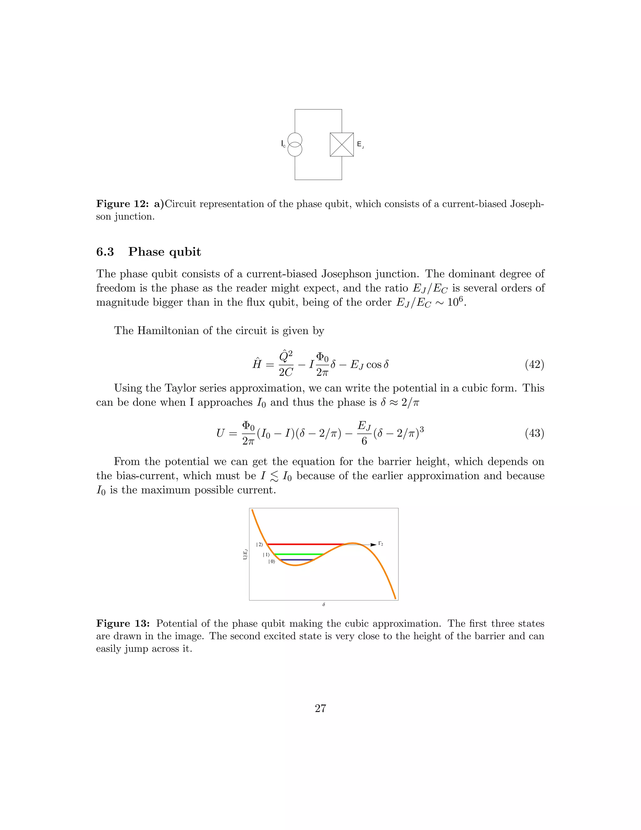
![∆U =
2
√
2Φ0I0
3π
1 −
I
I0
3/2
(44)
The approximated potential has one well because of its cubic nature. Instead, if we
plot the original potential, we get a tilted washboard potential with periodic wells. In the
well live three phase states, the second excited state’s energy being far enough to have a
two-level qubit approximation, but still not too widely separated. Due to the size of the
spacing, the state of the qubit can jump to the third level. Even if this might seem a
problem, it can be turned into an advantage in order to determine the state of the qubit.
∆
UE
J
Figure 14: Tilted potential of the phase qubit before the cubic approximation.
If we make a two-level approximation and reduce the Hamiltonian ignoring the rest of
the states, we get the reduced Hamiltonian[13]
Ĥqubit =
~ω01
2
σ̂Z +
r
~
2ω01C
σ̂X +
r
~ω01
3∆U
σ̂Z
!
(45)
To measure the quantum state of the qubit, a pulse with frequency (E2 − E1)/2 must
be applied. If the qubit is in the state |1i, it will be excited to the state |2i. When in
the state |2i it is probable to tunnel across the barrier. A voltage across the junction is
induced when the particle tunnels, therefore, measuring this voltage it is possible to deduce
the state of the qubit, being non-zero when the qubit is initially in the state |1i. On the
other hand, if the qubit is in the state |0i, nothing will happen, meaning that the measured
voltage will be null.
There is a different but similar way to measure the state of a phase qubit. The barrier
height in the potential can be controlled by the bias-current. It is possible to tilt the
potential allowing direct tunnelling from state |1i. Again, it will be possible to measure a
non-zero voltage when the qubit was in the state |1i and nothing will happen if it was in
the state |0i.
28](https://image.slidesharecdn.com/quantumcomputationwithsuperconductors-210425174826/75/Quantum-computation-with-superconductors-29-2048.jpg)
![7 Coupling of superconducting qubits
After achieving coherence times long enough to perform operations and readout on qubits,
the next step is implementing a two-qubit coupling, to then go adding more qubits to
build a quantum computer. Scalability in one of the main characteristics qubits should
have in order to build a quantum computer, as coupling of qubits is necessary for their
architecture. However, scalability to many qubits is still one of the goals before achieving
quantum computing.
The main purpose of coupling qubits is getting entangled states, because as we have
stated above, entanglement is one of the bases of quantum computation.When two qubits
are coupled, there are four entangled states, where the first and the second might be
degenerate. This states can be described using a 4x4 density matrix
ρ =
4
X
i=0
wi |ii hi| (46)
Where the energy states are linear combinations of the coupled qubit states
{|0, 0i , |1, 0i , |0, 1i , |1, 1i}
and wi is the weight of each state. The |01i and |10i are degenerate states having the same
energy.
One of the characteristics the coupling must have, is that it must be possible to turn the
coupling on and off when desired. When turned on, the coupling allows coherent transfer
of quantum states between the qubits.
Qubits can be coupled just by placing near each other, as they interact due to their
charge or flux. But this only allows coupling a qubit to its nearest neighbour. Coupling
to not neighbouring qubits is a condition for scalability making this system obsolete. The
simplest method to overcome this, is connecting all the qubits using an inductor L. This
way two not neighbouring qubits can be effectively coupled. If the frequency of the resulting
LC circuit ωLC is large enough, ~ωLC EJ , kBT, the fast oscillations couple the qubits
Hint =
X
ij
Ei
J Ej
J
EL
σi
yσj
y (47)
The interaction Hamiltonian of any two coupled qubits, performing a two-qubit oper-
ation gives[20]
Hint = −
E1
J
2
σ1
x −
E2
J
2
σ2
x +
E1
J E2
J
EL
σ1
yσ2
y (48)
29](https://image.slidesharecdn.com/quantumcomputationwithsuperconductors-210425174826/75/Quantum-computation-with-superconductors-30-2048.jpg)
![Another possibility is coupling the qubits capacitively. The most suitable method
should be chosen depending on each qubit.
For charge qubits, a scalable way of coupling them is connecting N Cooper-pair boxes
using an inductor L. Islands are coupled in parallel amongst them, and in series with a
dc-SQUID in each connection to the inductor. The two dc-SQUIDs connecting the CPB
to the circuit are identical, and all Josephson junctions in them have the same Josephson
energy and capacitance. To couple to particular qubits i and j the dc-SQUIDs connecting
this qubits must be switched on. The switching on and off condition is satisfied by the
dc-SQUID, which are easily switchable. Thus, the current through the inductor L has
contributions from all the coupled qubits. When all the Cooper-pair boxes are at their
degeneracy point, with their dc-SQUIDs also in the degeneracy point Φe = Φ0/2, except
one qubit i, the inductor is only connected to the ith island[21].
Two flux qubits can also be coupled by a superconducting loop surrounding them. A
change in the state of one qubit induces a current in the loop that induces itself a flux in the
other qubit. The loop is called a flux transformer. Flux transformers can be interrupted
by Josephson junctions, which enable to turn on or off the interaction between the qubits.
One device for such purpose is the dc-SQUID. The inductance between the qubits has two
components: that of the direct coupling between the qubits and the one of the coupling
through the dc-SQUID. The self-inductance of the dc-SQUID can be negative for certain
values of applied bias current and flux, having the opposite sign of the inductance of the
direct coupling between the qubits. This gives us the ability to switch the coupling off
when the inductances cancel each other, and on when they do not, tuning the coupling to
be stronger or weaker.
Figure 15: [5]Two flux qubits coupled by a dc-SQUID surrounding them.
A similar way to couple flux qubits inductively is to directly coupled them by sharing
one of the legs of the loop, as well as surrounded by a dc-SQUID as shown in Fig.15. The
energy eigenstates are similar to the classical states far from the flux degeneracy point.
Near the degeneracy point, the states are superpositions of the classical states due to
tunnel coupling[22].
30](https://image.slidesharecdn.com/quantumcomputationwithsuperconductors-210425174826/75/Quantum-computation-with-superconductors-31-2048.jpg)
![qubit a qubit b
coupler
Figure 16: Two flux qubits coupled by another flux qubit used as a coupler.
A variant of the method above is inductively coupling the flux qubits by inserting an
additional coupler loop between them as seen in Fig.16. The coupled qubits are three
Josephson junction loops, as well as the coupler. The coupler is connected to each loop
by one of its bigger junctions. The fluxes through the loops are controlled by the bias
currents. The coupling is switch on and off via the coupler’s flux bias, which tunes the
coupling strength[23].
Phase qubits are most commonly capacitively coupled. They can be directly connected
using a capacitance. The qubit bias currents are used to control the interaction between
them by tuning the energy level spacings of the junctions in and out of resonance. When
brought into resonance, the interaction produces an oscillation between the |01i and |10i
states lifting degeneracy. The strength of the coupling is set by the capacitive relation
Cc
Cc+CJ
, so the coupling strength is proportional to the coupling capacitance. Capacitive
coupling mixes the uncoupled states lifting the energy degeneracy[2][24].
31](https://image.slidesharecdn.com/quantumcomputationwithsuperconductors-210425174826/75/Quantum-computation-with-superconductors-32-2048.jpg)
![8 Logical operations with superconducting qubits
In the process of building a quantum computer, the purpose of coupling qubits to get
entangled states and the achievement of long4 coherent states is the manipulation of quan-
tum information via quantum gates. This quantum computer is built from a quantum
circuit composed of wires and quantum gates[25]. The wires carry around the quantum
information that is then manipulated by quantum gates. Quantum gates are operations
that transform qubit states. To understand how quantum gates can be achieved using the
previously studied superconducting qubits, first is necessary a theoretical introduction of
quantum gates.
8.1 Quantum gates
There are two types of quantum gates: single quantum gates, operated in a single qubit, and
multiple qubit quantum gates, operated in more than one qubit. A important characteristic
of quantum gates is that they must be invertible, so that there is no loss information, that
is, we can be able to know the input once we have the output. The quantum gates are
represented by matrices. The matrices U describing the gates must be unitary, that is, the
must satisfy
U†
U = I (49)
where U† is the adjoint of U and I is a unitary matrix. The constraint of being unitary
comes from the need to conserve the probabilities. This unitarity constraint of quantum
gates is the only constraint, any unitary matrix can be a quantum gate.
If we use the Bloch sphere, the unitary matrices correspond to rotations and reflections
of the sphere,
To illustrate the idea of a quantum gate, we will set the example of a NOT gate.
Classically, the NOT gate interchanges the 0 and 1 states, 0 → 1 and 1 → 0. The quantum
analogous of the classical NOT gate, the quantum NOT gate, operates linearly, as it must
transform the linear combination of the states |0i and |1i. Thus, if we have the state
α |0i + β |1i (50)
The NOT gate interchanges the states |0i and |1i obtaining
α |1i + β |0i (51)
As we have states above, quantum gates can be represented by matrices. We can write
the NOT gate using the matrix X
4
Of the order of microseconds
32](https://image.slidesharecdn.com/quantumcomputationwithsuperconductors-210425174826/75/Quantum-computation-with-superconductors-33-2048.jpg)
![X ≡
0 1
1 0
(52)
Notice that the matrix above is Pauli matrix σ̂X. We can also write the input state
(50) in vector notation
α
β
(53)
And thus we can write the quantum gate operation as a multiplication of the gate and
the input state
X
α
β
=
β
α
(54)
Apart from the NOT gate, there are many other important single-qubit gates. Like the
NOT gate, the other Pauli matrices represent quantum gates too
X ≡
0 1
1 0
; Y ≡
0 −i
i 0
; Z ≡
1 0
0 −1
(55)
Another important gate is the Hadamard gate, given by the matrix
H ≡
1
√
2
1 1
1 −1
(56)
This is one of the most useful single-qubit gates. The Hadamard gate turns |0i into
(|0i + |1i)/
√
2 and the |1i into |0i into (|0i − |1i)/
√
2. In the Bloch sphere picture, the
Hadamard gate is a rotation of 90 around the ŷ axis followed by a rotation of 180 around
the x̂ axis[1]. Another single-qubit gate, and the last one we will introduce is the phase
shift gate Φ, with matrix representation[26]
Φ ≡
1 0
0 eiφ
(57)
Besides the single-qubit gates, we have multiple-qubit gates. To perform multi-qubit
gates, entanglement amongst the qubits is essential. There are many multiple-qubit gates,
but here only the controlled-NOT or CNOT gate will be introduced. The CNOT gate is
the prototypical multi-qubit quantum logic gate. It has two input qubits: the control qubit
and the target qubit. If the control qubit is set to 0, then nothing happens to the target,
but if the control qubit is set to 1, the the target qubit’s state is switched
|00i → |00i ; |01i → |01i ; |10i → |11i ; |11i → |10i (58)
The matrix representation of the gate is[1]
33](https://image.slidesharecdn.com/quantumcomputationwithsuperconductors-210425174826/75/Quantum-computation-with-superconductors-34-2048.jpg)
![UCN ≡
1 0 0 0
0 1 0 0
0 0 0 1
0 0 1 0
(59)
Any multiple qubit logic gate can be composed from CNOT, Hadamard and phase
shift gates. This makes the set {H, Φ, CNOT} set a universal gate set, as any gate can be
performed from the composition of this gates alone[1].
8.2 CNOT gate using charge qubits
After studying how to couple superconducting qubits and introducing the basic theory
about quantum gates we are ready to perform a gate operation using superconducting
qubits. As the CNOT gate is a two-qubit gate we need to couple two qubits in order to
perform the gate operation. We will study the case where two charge qubits are coupled
by a capacitor. The (1) qubit will be the control qubit while the (2) qubit will be the
target qubit. The system has two pulse gates, to address each qubit individually. The
Hamiltonian of the system is given by
H =
X
N1,N2=0,1
EN1N2 |N1, n2i hN1, N2| −
EJ2
2
X
N2=0,1
(|0i h1| + |1i h0|) ⊗ |N2i hN2|
−
EJ1
2
X
N1=0,1
|N1i hN1| ⊗ (|0i h1| + |1i h0|)
(60)
where EJi is the Josephson energy of each qubit and EN1N2 = Ec1(Ng1 − N1)2 +
Ec2(Ng2 − N2)2 + Em(Ng1 − N1)(Ng2 − N2) is the total electrostatic energy of the system.
Eci are the charging energies of the islands and Em is the coupling energy. When Ng1
and Ng1 are far away from their degeneracy point 1/2 we have four independent entangled
states. If we fix one of the offset charges, Ng1 = C for example, our system is divided into
a pair of independent two-level systems |00i , |01i and |10i , |11i. The charging energies of
each of the two-level systems degenerate at different values of Ng2, Ng2L for |00i , |01i and
Ng2U for |10i , |11i. Applying a pulse in the control qubit shifts the system maintaining
Ng2 constant. If our input state is |00i and a pulse is applied, the system is brought to the
degeneracy point Ng2L, evolving with frequency Ω = EJ2
~ . Thus, the state of the system
evolves as
cos
Ω∆t
2
|00i + sin
Ω∆t
2
|01i (61)
so, if we send a π pulse, Ω∆t = π, we get the output state |01i. If we, on the other
hand, have the input state |10i and apply the same pulse, the system does not reach the
34](https://image.slidesharecdn.com/quantumcomputationwithsuperconductors-210425174826/75/Quantum-computation-with-superconductors-35-2048.jpg)
![degeneracy point Ng2U . IF Em remains large enough, the state remains almost unchanged.
Using the exact same method, we can perform the transition from |01i to |00i and suppress
the transition out of |11i. So, we have described a CNOT gate where the state of the target
qubit is flipped only when the state of the control qubit is |0i[27]. We can express this
operation using a matrix very similar to (59)
UCN ≡
0 1 0 0
1 0 0 0
0 0 1 0
0 0 0 1
(62)
35](https://image.slidesharecdn.com/quantumcomputationwithsuperconductors-210425174826/75/Quantum-computation-with-superconductors-36-2048.jpg)
![Bibliography
[1] M. A. Nielsen and I. L. Chuang. Quantum Computation and Quantum Information.
Cambridge, 2000.
[2] A. J. Berkley, R. C. Ramos, H. Xu, M. A. Gubrud, F. W. Strauch, P. R. Johnson,
J. R. Anderson, A. J. Dragt, C. J. Lobb, and F. C. Wellstood. Entangled macroscopic
quantum states in two superconducting qubits. Science, 300:1548–1550, 2003.
[3] B. Kraus. Quantum information Processing, Lecture Notes, chapter A5: Topics in
Quantum Information. Forschungszentrum Jülich GmbH, 2013.
[4] D. P. DiVincenzo. Quantum information Processing, Lecture Notes, chapter A1: Ori-
gins of Quantum Information Science. Forschungszentrum Jülich GmbH, 2013.
[5] J. Clarke and F. K. Wilhem. Superconducting quantum bits. Nature, 453:1031–1042,
2008.
[6] J.A. Schreier, A. A. Houck, J. Koch, D. I. Schuster, B. R. Johnson, J. M. Chow, J. M.
Gambetta, J. Majer, L. Frunzio, M. H. Devoret, S. M. Girvin, and R. J. Schoelkopf.
Suppressing charge noise decoherence in superconducting charge qubits. Physical Re-
view B, 77:180502(R), 2008.
[7] S. M. Girvin. Circuit q.e.d.: Superconducting qubits coupled to microwave photons.
In J.M. Raimond, D. Esteve, and J. Dalibard, editors, Les Houches Summer School
Series, 2003.
[8] J. Q. You and F. Nori. Superconducting circuits and quantum information. Physics
Today, 58:42–47, 2005.
[9] M. H. Devoret and R. J. Schoelkopf. Superconducting qubits for quantum information:
an outlook. Science, 339:1169–1174, 2013.
[10] D. J. Van Harlingen, T. L. Robertson, B. L. Plourde, and J. Clarke. Decoherence
in josephson-junction qubits due to critical current fluctuations. Physical Review B,
70:064517, 2004.
[11] L. Faoro and L. B. Toffe. Microscopic origin of low frequency flux noise in josephson
circuits. arXiv:0712.2834v1, 2013.
[12] Y. Nakamura, Y. A. Pashkin, and J.S. Tsai. Coherent control of macroscopic quatum
states in a single-cooper-pair box. Nature, 398:786–788, 1999.
[13] M. H. Devoret, A. Wallraff, and J. M. Martinis. Superconducting qubits: A short
review. arXiv:cond-mat/0411174, 2004.
37](https://image.slidesharecdn.com/quantumcomputationwithsuperconductors-210425174826/75/Quantum-computation-with-superconductors-38-2048.jpg)
![[14] M. H. Devoret. Quantum fluctuations in electrical circuits. In J.M. Raimond, D. Es-
teve, and J. Dalibard, editors, Les Houches Summer School Series, 1995.
[15] V. Bouchiat, D. Vion Vion, P. Joyez, D. Esteve, and M. H. Devoret. Quantum coher-
ence with a single cooper pair. Physica Scripta, T76:165–170, 1998.
[16] J. M. Gambetta. Quantum information Processing, Lecture Notes, chapter B4: Con-
trol of Superconducting Qubits. Forschungszentrum Jülich GmbH, 2013.
[17] S. M. Girvin, M. H. Devoret, and R. J. Schoelkopf. Circuit q.e.d. and engineering
charge-based superconducting qubits. Physica Scripta, T137:014012, 2009.
[18] J. Koch, T. M. Yu, J. Gambetta, A. A. Houck, D. I. Schuster, J. Majer, A. Blais,
M. H. Devoret, S. M. Girvin, , and R. J. Schoelkopf. Charge insensitive qubit design
derived from the cooper pair box. arXiv:cond-mat/0703002v2, 2007.
[19] V.E. Manucharyan. Quantum information Processing, Lecture Notes, chapter D1:
Fluxonium qubit. Forschungszentrum Jülich GmbH, 2013.
[20] Y. Makhlin, G. Schön, and A. Shnirman. Josephson-junction qubits with controlled
couplings. Nature, 398:305–307, 1999.
[21] J. Q. You, J.S. Tsai, and F. Nori. Scalable quantum computing with josephson charge
qubits. Physical Review Letters, 89:197902, 2002.
[22] J. B. Majer, F. G. Paauw, A. C. J. ter Haar, C. J. P. M. Harmans, and J. E. Mooij.
Spectroscopy on two coupled superconducting flux qubits. Physical Review Letters,
94:090501, 2005.
[23] S. H. W. van der Ploeg, A. Izmalkov, A. M. van den Brink, and A. Zagoskin. Con-
trollable coupling of superconducting flux qubits. Physical Review Letters, 98:057004,
2007.
[24] M. Steffen, M. Ansmann, R. C. Bialczak, N. Katz, E. Lucero, R. McDermott, M. Nee-
ley, E. M. Weig, A. N. Cleland, and J. M. Martinis. Measurement of the entanglement
of two superconducting qubits via state tomography. Science, 313:1423–1425, 2006.
[25] R. Barends, A. Shabani, L. Lamata, J. Kelly, A. Mezzacapo, U. Las Heras, R. Bab-
bush, A. G. Fowler, B. Campbell, Yu Chen, Z. Chen, B. Chiaro, A. Dunsworth,
E. Jeffrey, E. Lucero, A. Megrant, J. Y. Mutus, M. Neeley, C. Neill, P. J. J. O’Malley,
C. Quintana, P. Roushan, D. Sank, A. Vainsencher, J. Wenner, T. C. White, E. Solano,
H. Neven, and John M. Martinis. Digitized adiabatic quantum computing with a su-
perconducting circuit. Nature, 534(7606):222–226, 06 2016.
[26] D. Bruss. Quantum information Processing, Lecture Notes, chapter A2: Introduction
to Quantum Information. Forschungszentrum Jülich GmbH, 2013.
38](https://image.slidesharecdn.com/quantumcomputationwithsuperconductors-210425174826/75/Quantum-computation-with-superconductors-39-2048.jpg)
![[27] T. Yamamoto, Y.A. Pashkin, O. Astafiev, Y. Nakamura, and J. S. Tsai. Demonstration
of conditional gate operation using superconducting charge qubits. Nature, 425:941–
944, 2003.
[28] D. V. Averin and C. Bruder. Variable electrostatic transformer: controllable coupling
of two charge qubits. Physical Review Letters, 91:057003, 2003.
39](https://image.slidesharecdn.com/quantumcomputationwithsuperconductors-210425174826/75/Quantum-computation-with-superconductors-40-2048.jpg)

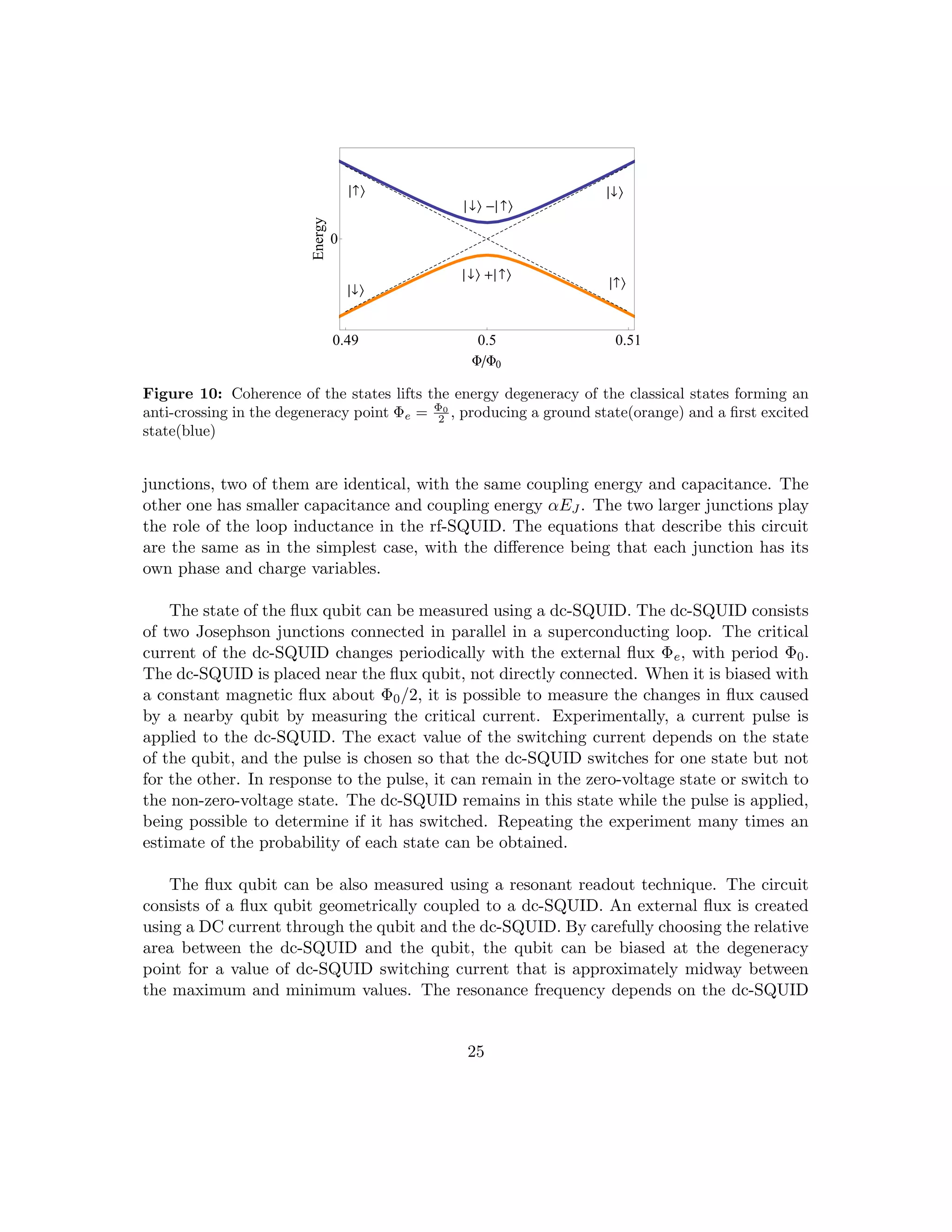
This document describes a student's graduation project on using superconducting circuits for quantum computation. It provides an introduction to the topic and outlines the structure of the project. The project will first introduce the concept of a qubit and basics of quantum computation. It will then describe different types of qubit technologies before focusing on superconducting circuits. The document will explain the necessary quantum phenomena like coherence and noise. It will explore superconducting qubits in detail and how to couple them. Finally, it will demonstrate how to perform logical operations using superconducting qubits.


![Vibe Coding vs. Spec-Driven Development [Free Meetup]](https://cdn.slidesharecdn.com/ss_thumbnails/vibecodingvsspecdrivendevelopment-251209105622-43f455e7-thumbnail.jpg?width=640&height=640&fit=bounds)


