SlideShare a Scribd company logo
1 of 20
Download to read offline
“…it seems that the laws of physics present no barrier
to reducing the size of computers until bits are the size of atoms,
and quantum behavior holds dominant sway.”
—R. P. Feynman, 1985
Quantum computation requires
a very special physical
environment. Numerous
operations must be performed on the
quantum states of the qubits (or quan-
tum bits) before those states decohere,
or lose the interlocking phase relation-
ships that give quantum computation
its power. Thought to be an unavoid-
able outcome of the interaction
between the quantum state and the
environment, decoherence threatens
the life of a quantum system.
Any attempt at building a real
quantum computer therefore leads to
what some scientists refer to as the
yin-yang of quantum computation:
On the one hand, the qubits must
interact weakly with the environment
in order to limit decoherence. On
the other hand, they must be easily
accessible from the outside and must
interact strongly with each other, or
else we could not manipulate the
Ion-Trap Quantum Computation
Michael H. Holzscheiter
264 Los Alamos Science Number 27 2002
quantum state, implement quantum
algorithms, and read out the result of
a calculation in a timely fashion.
How can we hope to meet such con-
tradictory goals?
Ion-trap quantum computers, as
originally proposed by Ignacio Cirac
and Peter Zoller (1995), offer a possi-
ble solution to this dilemma. As its
name implies, an ion trap confines
charged particles to a definite region of
space with magnetic and electric fields.
In a specific realization of such a trap,
called a linear radio-frequency quadru-
pole (RFQ) trap, or a linear Paul trap
(Raizen et al. 1992, Walther 1994),
time-varying electric fields are used to
hold a line of ions in place—like pearls
on a string. These ions serve as the
physical qubits of the quantum com-
puter. Immobilized by the trapping
fields and confined inside an ultrahigh
vacuum chamber, they are effectively
isolated from the environment.
However, by addressing individual ions
with sharply defined laser beams, we
can initialize the computer, control the
qubit states during the operation of
logic gates, and read out the results at
the end of the computation. The inter-
action between the individual ions is
mediated by the Coulomb force
between the charged particles.
This article discusses the design
principles for isolating single ions in a
linear Paul trap (Paul et al. 1958),
whose operational principles are
described in detail. The individual ele-
ments of an ion-trap computer will be
introduced, and how to initialize,
manipulate, and interrogate the qubits
will be explained. Specific schemes
that were implemented in the quantum
computation project at Los Alamos
(Hughes et al. 1998) will illustrate the
descriptions. Ion-trap quantum compu-
tation is rapidly evolving, and numer-
ous groups around the world are
developing new ideas and experimen-
tal techniques. The reader will get a
flavor of this activity in the last section
of the article, which summarizes sev-
eral important results achieved within
the last few years: the on-demand cre-
ation of entangled states of up to four
ions by the National Institute of
Science and Technology (NIST) group
in Boulder, Colorado; the development
of a novel cooling scheme by a group
at the University of Innsbruck, Austria,
which would allow researchers to
quickly cool large numbers of trapped
ions with drastically reduced opera-
tional overhead; and the construction
of an effective defense against the
forces of decoherence.
The Physics of Ion Traps
Two basic types of devices can
confine charged particles to well-
defined regions of free space: Penning
traps and Paul traps. The Penning
trap, which was primarily developed
by Hans Dehmelt at the University of
Washington in Seattle, uses a strong
magnetic field and a static electric
field to create a nearly perfect three-
dimensional, harmonic trapping
potential (Dehmelt 1967). Some of the
most precise tests of fundamental
physical symmetries to date have been
conducted with this device, whose
operating principles are described in
the box “The Penning Trap” on the
next two pages.
Although Penning traps nicely
solve the fundamental problems of
ion confinement, so far they have not
been used for quantum computation.
The trap’s strong magnetic field
causes ions to move rapidly in a
circle (the cyclotron motion dis-
cussed in the box), whereas we want
the physical qubits to have as little
motion as possible. That is why the
favored trap for quantum computa-
tion is the Paul trap, in which there
is no magnetic field and oscillating
electric fields (as opposed to static
ones) confine the ions. This device
was invented by Wolfgang Paul from
the University of Bonn in Germany,
who shared the 1989 Nobel Prize in
physics with Dehmelt.
Paul enjoyed telling the following
anecdote about how he hit upon the
idea for his device. Germans like soft-
boiled eggs for breakfast, and on a
particular Sunday morning, Paul had
prepared two eggs of different sizes
and had placed them on a serving tray.
When he started to walk, tray in hand,
toward the bedroom to surprise his
wife with breakfast in bed, the eggs
began to roll. He counteracted their
motion by shaking the tray and was
able to confine the larger egg to the
center by shaking with a particular
frequency and amplitude. (It was cer-
tainly not a well-defined harmonic
shaking.) The smaller egg, however,
kept rolling toward the edge, so Paul
changed amplitude and frequency and
successfully prevented this egg from
falling, at the expense of allowing the
larger one to wobble toward the edge.
Whether he ever reached the bedroom
with both eggs on the tray and enjoyed
a leisurely breakfast with his wife
remains unknown, but that morning
Paul realized not only the basic princi-
ple of the RFQ trap but also the mass-
selective feature of such an instrument.
At that time, he was keen on develop-
ing a mass filter for ions, that is, a
two-dimensional structure that could
transmit an ion with a specific
charge-to-mass ratio and not any other
ratio. Eventually, Paul’s idea was used
to generate three-dimensional, mass-
selective confinement systems, but
Cirac and Zoller returned to the origi-
nal two-dimensional structure and
proposed using it as the basis for a
quantum computer.
The Linear Paul Trap. To under-
stand the linear RFQ trap, consider a
positively charged ion floating in free
space and surrounded by four infi-
nitely long conducting rods, as shown
in Figure 1. We can give one pair of
opposing rods a positive charge and
the other pair a negative charge
Number 27 2002 Los Alamos Science 265
Continued on page 268
+
+
+
Capacitor plate
B-field line
+
+
+
Capacitor plate
266 Los Alamos Science Number 27 2002
Ion-Trap Quantum Computation
The Penning Trap
Decades before individual ions were considered as candidates for qubits in a
quantum computer, experimental physicists were challenged to realize a simpler
Gedanken, or thought, experiment embodied by the statement often made by
theorists: “Consider a single (silver) ion in a uniform magnetic field” (Tanoudji
et al. 1977). Thought became reality in 1973, when Hans Dehmelt and his col-
leagues at the University of Washington in Seattle were able to capture a single
charged particle in a Penning trap. The ion that drifted into the central region of
that device was trapped by a strong, uniform magnetic field and by the electro-
static field produced by a set of specially shaped electrodes. The entire device
operated under ultrahigh vacuum to limit the interactions between the ion and
the background atoms.
The University of Washington group refined the technique and used the trap to
confine a single electron (Wineland et al. 1973) and later a single barium ion,
using an RFQ Paul trap (Neuhauser et al. 1980), and performed precision spec-
troscopy on these systems. The special arrangement of fields caused the single
electron to behave as if it were bound to a nucleus for it displayed a set of
energy levels, or excited states, similar to those of the hydrogen atom. Dehmelt
therefore named his electron in a Penning trap “geonium—a single electron
bound to Earth.” The artificial geonium “atom” was, in a sense, closer to per-
fection than a real atom. The spacing between energy levels was nearly con-
stant because it reflected the trap’s nearly perfect harmonic-oscillator potential.
Dehmelt and coworkers used geonium to perform some of the most precise
tests of fundamental symmetries. In a more mundane fashion, Dehmelt called
the ion ASTRID (for “a single trapped ion dancing”). (Perhaps, if you keep an
ion or electron for such a long time, you may become attached to it.)
To understand the operating principles of the Penning trap, consider a charged
particle (ion) moving freely in space. To confine it to a specific spot in space,
we can apply electrical forces to its charge. If we place the ion between two
parallel conducting plates that are charged to an electric potential of the same
sign as the ion, the Coulomb repulsion will keep the particle from moving
closer to either plate (see Figure A).
The ion can still move in directions parallel to the conductors. We can try
to remove all escape routes by placing more conductors around the particle.
But Michael Faraday discovered more than 150 years ago that an electric field
cannot penetrate a closed metal enclosure—hence, the penchant for science
museums to place a person inside a “Faraday cage” that is then exposed to
violent lightning bolts. The courageous volunteer remains unharmed because
the lightning’s electric field vanishes inside the cage. Similarly, if we fully
enclose our particle in a cage of conducting plates, the electric field disappears,
and we lose the forces holding the particle from the walls.
A more successful approach is to use the fact that an electric charge moving in
a magnetic field will experience a force perpendicular to the direction of both
the magnetic field and the particle’s velocity (the Lorenz force F = qv × B).
Therefore, if we apply a magnetic field perpendicular to our parallel conducting
plates (see Figure B), we force the ion onto a circular path around the magnetic
field line, closing off the sideway escape routes.
Figure A. Electrostatic Forces
The positively charged particle is
repulsed by the capacitor plates but is
free to move anywhere in the horizontal
plane.
Figure B. Applying a Magnetic
Field
A magnetic field causes the ion to circle
around a field line (cyclotron motion),
thus confining the ion in the horizontal
plane.
Whereas the system shown in Figure B can confine charged particles (and has
been used for a number of experiments), the special character of the Penning
trap is given by the clever shaping and arrangement of the electrodes. As shown
in Figure C, two end caps shaped as hyperbolae of revolution replace the paral-
lel plates, and a ring-shaped center electrode defines the electrostatic potential
on the edge of the trap.
The arrangement shown in Figure C not only leads to perfect confinement of
individual charged particles but also allows the motion of a trapped particle to
be separated into three independent harmonic motions. In order of decreasing
frequency, the three motions are (1) the fast “cyclotron” motion of the charge
around the magnetic field lines, (2) a slower oscillation in the direction of the
magnetic field that is due to the electrostatic repulsion from the two end caps,
and (3) a much slower drift motion that is due to the crossed electric and mag-
netic fields (see Figure D).
The drift motion is easily understood if one focuses on the cyclotron motion.
The positively charged particle is accelerated toward the negatively charged
ring electrode as it moves away from the electrical center of the trap. This
acceleration increases the radius of curvature for the outer half of the cyclotron
motion. As the particle moves back toward the center during the second half of
the cyclotron motion, it decelerates, and the radius of curvature decreases. The
net effect is a distortion of the circular cyclotron motion into a spiral that bends
around the electrical center of the trap, as seen in Figure E.
The harmonic motions account for the almost constant spacing between energy
levels in Dehmelt’s geonium atom, but this orderliness is hardly noticeable in
the roller-coaster-like motion of a trapped particle. If you actually want to expe-
rience the particle’s motion yourself, there is a carnival ride in which these
three components of motion are present—but watch your stomach!
Number 27 2002 Los Alamos Science 267
Ion-Trap Quantum Computation
Figure D. Motion in the Penning
Trap
The three-dimensional motion of an ion
in the trap consists of three harmonic
motions: a fast cyclotron motion, a
slower up-down oscillation, and a slow
circular drift motion.
B
E
Distorted
cyclotron
motion
E × drift
motion
+
B
Axis of
symmetry
B-field
arrow
+
Trapping
region
–
Figure C. The Penning Trap
The two endcaps, which are hyperbolae
of revolution, replace the flat capacitor
plates. The central ring electrode helps
define the harmonic potential at the
center of the trap.
Figure E. Drift
Schematic of the drift motion that
results from the crossed electric (E)
and magnetic (B) fields.
(relative to some arbitrary “zero”
potential).1 The positive ion feels a
repulsive force from the positively
charged conductors and is pushed
toward the center of the trap. The ion
simultaneously feels an attractive
force due to the negatively charged
conductors and is pulled outwards.
If we now reverse the polarity of
our four electrodes, interchanging
plus for minus and minus for plus,
the ion’s motion will begin to
reverse. Where it was moving out, it
will now be moving in, and vice
versa. However, if the reversal takes
place quickly, the “heavy” ion
cannot easily respond; it has too
much inertia to follow the fast
changes in the electric field exactly.
Instead, the ion will respond to
the time-averaged electric field.
If we switch the polarity of the
electrodes at a few megahertz
(or a few million times a second)
by applying a radio-frequency (rf)
voltage and if the amplitude is
correct, then the time-averaged field
generates a harmonic pseudopoten-
tial with its minimum located at
the trap axis. The ion is pushed to
the bottom of the pseudopotential
268 Los Alamos Science Number 27 2002
Ion-Trap Quantum Computation
Figure 1. Principles of the Linear Paul Trap
(a) The linear Paul trap consists of four conducting rods.
Two opposing rods are connected to one pole of a radio-
frequency (rf) voltage source, whereas the remaining two are
connected to the other pole. The axis of symmetry between
the rods is the trap axis. (b) With the rods charged as shown,
the resulting electric force pushes a positive ion to the nega-
tive rods and repels it from the positive ones. (c) Half an rf
period later (see graph below), the polarity of all rods is
reversed, and the direction of the force also reverses.
(d) If the polarity changes fast enough, a heavy ion becomes
stuck in a rapid back-and-forth motion. Because the electric
fields are at a minimum at the trap axis, an effective force
pushes the ion toward the center, where it becomes trapped
(although it is still free to move along the axis). The blue
dots seen between the rods in part (a) represent a string
of radially trapped ions. The string can be confined axially
when a positively charged electrode (end cap) is placed at
each end of the rods.
rf
+
+
–
–
rf
+/–
rf
(b) t = t
1
(a)
(d) Time Average
+
+
–
–
rf
(c) t = t
2
+/–
+/–
+/–
rf
Voltage
+
–
0
t1
Time
rf
Voltage
+
–
0
t2
Time
rf
Voltage
+
–
0
Time
1 For reasons discussed on the previous
two pages, all four conductors cannot be
positively charged, or the electric fields
within the trap would disappear.
Continued from page 265
well and becomes trapped forever—
at least in principle—near the center.
To generate the mass selectivity
sought by Paul, we add a positive
direct-current (dc) component to the
rf voltage. Positive ions outside a cer-
tain mass range feel less of a restoring
force from the pseudopotential and
are kicked out of the trap by the repul-
sive dc field. This technique is one of
several that we can use to preferen-
tially retain qubit ions instead of, say,
a residual gas ion that may be present
in the ultrahigh vacuum trap.
Of course, the ion’s motion is still
unrestricted in the direction parallel to
the trap’s axis. For confinement in this
third dimension, we simply add an
electric dc potential to a pair of “end
electrodes” that are on either side of
the region of interest. This axial field
plugs up the escape route along the
symmetry axis of the system, and
the ion becomes trapped in three
dimensions. By substantially reducing
the ion’s energy (cooling), we coax
the ion into lying along the central
portion of the trap axis, where the
radial and axial confining potentials
are at a minimum. If several very cold
ions are in the trap, then they all fall to
the center, and the mutual Coulomb
repulsion between the ions causes
them to line up neatly along the axis.
Motion in the Trap. Although the
combination of rf and dc fields within
the trap drives the ion into a complex
radial motion, that motion is fully
described by a set of differential equa-
tions called “Mathieu’s Equations.”
The bound solutions of those equa-
tions yield a stability diagram that
allows one to evaluate the effective-
ness of the trap, given the values of
several critical parameters, such as the
amplitudes of the rf and dc compo-
nents of the voltage, the rf, the ion
mass, and the size of the trap
(Dawson 1976).
As long as we keep the values of
the critical operational parameters
within certain ranges, an ion will
remain bound to the axis of the device.
Furthermore, the magnitude of the
restoring force of the pseudopotential
holding the ions in the radial direction
will remain directly proportional to
the distance from the center—the
hallmark of a harmonic potential.2
In other words, to a good approxima-
tion, the ions will undergo harmonic
oscillations in the radial direction with
frequency ωr (or with frequency ωx
and ωy in case the potential is different
in the x- and y-directions). This motion
is commonly referred to as the secular
motion.
The ions’ motion can become dis-
torted if the minima of the rf field and
the pseudopotential are misaligned
within the trap. Misalignment can
occur because of some small asymme-
try in the trap’s construction or
because of small dc patch potentials
on the electrode surfaces. Regardless
of the reason, misalignment will cause
the ions to lie “off center” (that is, off
the line where the rf field vanishes).
Those ions will experience the strong
gradient of the rf field and undergo
rapid oscillations—at the frequency of
the applied rf field—around their
time-averaged equilibrium position.
This so-called micromotion is the
main source of ion heating. We can
suppress the micromotion by adding a
compensating dc voltage to some of
the rf electrodes (or to auxiliary con-
trol electrodes) and thereby shift the
ions’ positions closer to the actual rf
center.
In addition to exhibiting secular
motion and the unwanted micromo-
tion, an ion or, more important, a
string of ions will also vibrate in the
axial direction. The motion will be
harmonic because the dc voltage on
the end electrodes creates a harmonic
potential along some length of the
trap axis. The vibrations are similar to
those exhibited by a set of pendula
connected to each other by springs;
the swinging of one pendulum sets the
others in motion (see Figure 2).
Unlike vibrations of classical pendula,
however, the vibrations exhibited by a
string of ions are quantized; that is,
the amplitude of the motion depends
on the number of quanta (phonons) in
the vibrational mode.
For N ions in a trap, there are
N axial vibrational modes and an
additional 2N modes for motions
transverse to the axis. Each mode has
a distinct vibrational frequency. The
lowest-frequency (lowest-energy)
vibration is the so-called common
mode, in which the ions oscillate back
and forth in unison along the axis.
This mode figures heavily in the origi-
nal quantum-computing scheme of
Cirac and Zoller. Because all ions
participate in the common-mode
oscillation, when we add (or remove)
a quantum of energy to this motion by
interacting with one of the ions, we
influence all other ions in the string.
Any two qubits, regardless of the dis-
tance between them, can therefore be
coupled together to perform logic
operations.
Other proposals make use of some
of the higher-frequency modes to
couple qubits together (James 1998a).
These modes have more-complex
vibrational patterns and relatively
higher excitation energies than the
common mode, but it still takes very
little energy to excite them. Even a
string of very cold ions will vibrate
in some intricate expression of the
various modes, a problem that is
addressed in the discussion of ion
cooling.
If only a few ions are confined in
the trap, the ions will align themselves
linearly along the axis. But increasing
the number of ions or increasing the
dc voltage applied to the end elec-
trodes introduces instabilities because
Number 27 2002 Los Alamos Science 269
Ion-Trap Quantum Computation
2 To generate a pure harmonic potential,
the four electrodes should have hyperbolic
cross sections, but in practice we approxi-
mate that ideal shape with cylindrical rods.
the ions are effectively squeezed
closer together. The Coulomb
repulsion between neighboring ions
becomes stronger than the radial
restoring force, and the ions start
buckling out into a zigzag pattern.
When even more ions are added, the
zigzag pattern develops into a com-
plex three-dimensional helical struc-
ture (Raizen et al. 1992, Walther
1991, 1994). Some of the ions will
move away from the axis and will
experience the strongest micromotion
heating—a situation clearly to be
avoided. We have studied this transi-
tion from linear to three-dimensional
structures in some detail (Enzer et al.
2000) and have quantified the parame-
ter space available for quantum
computing in a linear RFQ ion trap.
Elements of the Ion-Trap
Quantum Computer
In 1994, inspired by the great suc-
cess of ion traps in the field of preci-
sion measurements, Cirac and Zoller
proposed that the RFQ ion trap had
the right characteristics to support the
long sequence of precision operations
required for quantum computation.
A string of ions trapped along the
symmetry axis of the trap would be
the quantum register of the computer.
Each ion could be addressed by
tightly focused laser beams, initial-
ized to an arbitrary state, manipu-
lated, and then probed at the end of a
calculation. Most important, the isola-
tion from the environment afforded
by the trap would allow for long
coherence times.
One- and Two-Qubit Operations.
The logical qubit states |〉 and |〉 of
the ion-trap quantum computer must
be defined as they always are for any
quantum computer. (To stress that the
 and  used to designate the states
are notational and have no numerical
meaning, we have used a font differ-
ent from the one for the numbers 0
and 1.) We simply identify the ion’s
electronic ground state with the qubit
state |〉 and a long-lived excited state
with the qubit state |〉.
We also want to apply a unitary
transformation to a single qubit,
that is, to implement a one-qubit gate,
and rotate the qubit in Hilbert space
to an arbitrary superposition of the
|〉 and |〉 states. (Two-level systems
and the rotation of a qubit in Hilbert
space are discussed in the article
“Quantum Information Processing”
on page 2.) To do so, we subject the
ion to a laser pulse of a specific
amplitude, frequency, and duration.
Assuming the ion is in its ground
state, the laser pulse will cause the
electron wave function of the target
ion to evolve to some superposition
of the ground and excited states. (We
cause the electron to undergo part of
a Rabi oscillation.) Illuminating the
ion with a so-called π-pulse, for
example, will evolve the electron
wave function through half a Rabi
oscillation period and leave the ion in
the excited state. The qubit would
have rotated from the |〉 to the |〉
state. If the duration of the pulse is
halved (a so-called π/2-pulse), the ion
would be left in an equally weighted
superposition of the ground and
excited states. The qubit would have
rotated to the 1/√2(|〉 + |〉) state.
270 Los Alamos Science Number 27 2002
Ion-Trap Quantum Computation
Figure 2. Vibrational Modes
A set of strongly coupled pendula can be used to envision the vibrational motion of
a string of ions in a harmonic potential. These vibrational modes affect all ions
simultaneously. If we set any one of the pendula in motion, the others will move.
Similarly, if we grab hold of any pendulum and stop it, all others will stop. (a) The
common mode (center-of-mass mode), in which all pendula swing one way and then
the other, has the lowest frequency (lowest energy) of all modes. Using this mode
to couple two qubits together in the trap is the basis of the Cirac-Zoller proposal.
(b) The breathing mode, in which pendula at opposite ends move in opposite direc-
tions, has the next highest frequency. For an odd number of pendula, the middle
one does not move. This mode is less susceptible to heating by external noise
sources and has also been used to couple qubits. (c) Shown here is another higher-
order mode. In an ion trap, the ions can vibrate in three dimensions; for N trapped
ions, there are 3N vibrational modes.
(a) Common Mode
(b) Breathing Mode
(c) Higher-Order Arial Mode
While we can use laser pulses to
interact with each qubit separately
(and excite a qubit’s electronic, or
internal, degrees of freedom), we can
also use another laser to excite the
trap’s vibrational modes and hence to
interact with all qubits simultaneously.
The latter process can be viewed as
interacting with the qubits’ external
degrees of freedom. The state of a
string of j qubits in the trap is there-
fore explicitly given as
|q1, q2, … qj〉|n〉 . (1)
The first ket, |q1, q2, … qj〉, refers to
the logical qubit states, with qj =  or
. The second ket, |n〉, refers to the
common-mode vibrational state, and
the value of n, say, 0, 1, 2, …, indi-
cates the number of phonons in the
common mode. (Although the string
of qubits may initially be in another
mode, we will restrict our attention to
the common mode.) Thus, in the state
|q1, q2, … qj〉|0〉 , (2)
the ions are not vibrating because
there are no phonons in the common
mode. In the state
|q1, q2, … qj〉|1〉 , (3)
the common mode contains one
phonon and all the ions are swaying
in unison along the trap axis.
As mentioned earlier, the common
mode is used as a “bus” that couples
different ions together. To better
understand this coupling, consider
first that the frequency of the transi-
tion between the |〉 state and the |〉
state is ω0, and that the common-
mode vibrational frequency ω1 is
much lower than ω0. Similar to the
case of two coupled harmonic oscilla-
tors, the energy spectrum of the ion
exhibits resonances not only at the
“carrier” frequency ω0, but also at the
“sideband” frequencies ω0 ± ω1 (see
Figure 3). The resonance with the
higher frequency is commonly known
as the blue sideband; the one with the
lower frequency, as the red sideband.
For cold ions, the linewidth ∆ω0 of
the carrier transition is very narrow3
and is less than the energy difference
between the carrier and either side-
band. Thus, the sidebands and the car-
rier can be resolved within the cold
ion’s frequency spectrum.
Now consider, for example, a pro-
cedure used to place two ions in an
entangled state. Assuming that the
ions are initially in the state |〉|0〉,
if we were to address the first ion
with a π-pulse from a laser detuned to
the blue sideband of the internal tran-
sition, both the internal and external
states of that ion would be excited.
Because an excitation in the common
mode is felt by both ions, the result
would be the two-qubit state |〉|1〉.
If, instead, we address the first qubit
Number 27 2002 Los Alamos Science 271
Ion-Trap Quantum Computation
Energy
n – 1〉 n〉 n + 1〉
Red Blue
Carrier
Common-mode vibrational states
0 – 1 0 0 + 1
(a) Resolved Sideband Structure
Carrier transition
Red sideband Blue sideband
(b) Resonant Transitions
〉n〉 →〉n – 1〉 〉n〉 →〉n + 1〉
〉n〉 →〉n〉 〉
〉
ω ω ω ω ω
Figure 3. Vibrational Sideband Spectrum
(a) An ion trap naturally couples an ion’s electronic excitations to its vibrational motion. Each electronic transition at resonant
frequency ω0, known as the carrier frequency, is therefore accompanied by other sideband transitions. We show the two side-
bands closest in frequency to the carrier: the lower-energy red sideband at frequency (ω0 – ω1), and the higher-energy blue side-
band at frequency (ω0 + ω1). A laser with a sufficiently narrow linewidth can interact with the ion via a specific sideband or the
carrier. (b) Interacting with a particular qubit (ion) via a sideband transition will change the qubit’s internal state and simultane-
ously the external state of all the qubits in the trap, either increasing the number of phonons in the common mode by one (exci-
tation on the blue sideband) or decreasing the number by one (excitation on the red sideband).
3 The metastable excited state has a very
long lifetime, which leads to a narrow
linewidth according to Heisenberg’s
uncertainty principle. To take an example
from the Los Alamos experiment, a cal-
cium ion excited to the 32D3/2 state will
decay to the ground state only after an
average delay of about 1 second, which
results in a transition linewidth of about
1 hertz.
with a π/2-pulse (see Figure 4), both
qubits are placed in a superposition of
the two states, namely,
1/√2(|〉|0〉 + |〉|1〉) . (4)
We then address the second ion
(which is still in its ground state)
with a π-pulse tuned to the red side-
band. The laser energy is too low to
excite directly the ground-to-excited-
state electronic transition, but the
transition still occurs if extra energy
can be taken from the common
mode. The end result is that all
phonons have been removed from
the quantum register at the end of the
operation, and we create a two-qubit
entangled state:
1/√2(|〉 + |〉)|0〉 . (5)
We can no longer describe the system
as individual ions being in the ground
or the excited state. The result of a
measurement on one ion is strongly
correlated to the status of the other
ion. Notice that this procedure works
equally well if one or more ions are
placed in between the first and second
ions because the excitation of the
common mode is shared by all ions.
Besides defining the individual
operations just described, Cirac and
Zoller also spelled out in detail the
steps needed to perform a “controlled-
not” (cnot) gate. In such an operation,
a “target qubit” flips its state only if a
second qubit, the “control qubit,” is
originally set to its logical |〉 value.
Dave Wineland’s group at NIST first
implemented the cnot gate in an ion
trap in 1995 (Monroe et al. 1995),
albeit using only a single ion in the
trap. (The two states of the control
qubit were the two lowest-energy trap
vibrational states.) Still, because any
computation can be performed with a
number of two-qubit cnot gates,
together with some single-qubit gate
operations, the realization of a cnot
gate in a quantum computer is an
important benchmark.
Readout. At the end of any quan-
tum calculation, the individual qubits
in the quantum register will be in
defined states, which must be read out
with high fidelity. A powerful readout
tool makes use of the phenomenon of
quantum jumps (Sauter et al. 1986,
Bergquist et al. 1986). The readout
method is easily understood when one
examines the generic ion-level scheme
272 Los Alamos Science Number 27 2002
Ion-Trap Quantum Computation
The vibrational state is indicated by the position of the ions
on the rungs of a ladder in the harmonic potential well. In
this diagram, the electronic ground state of an ion is indi-
cated by a solid circle; the excited state, by an open circle.
(a) Suppose two qubits are initialized to the state |

〉|0〉.
Addressing the first qubit with a π-pulse from a laser tuned
to the blue sideband will excite the ions to the state |

〉|1〉.
The first ion is in its electronic excited state, while the
second remains in its electronic ground state. Because
the common mode affects all ions, both ions are excited
to the |n = 1〉 vibrational state. (b) Two qubits can be
entangled if we illuminate the first qubit with a π/2-pulse on
the blue sideband. The ions are placed in a superposition of
states: 1/√2(|

〉|0〉 + |

〉|1〉). If the second ion is then illumi-
nated by a π-pulse from a laser tuned to the red sideband,
it can absorb the photon only if energy is available from
the vibrational mode. Thus, ion 2 is excited only if ion 1
was excited; it remains in the ground state if ion 1 was in
the ground state. The two-ion system therefore exhibits
the strong correlation of observables, which according to
Bohr, define the condition of entanglement. The end result
of the operation is the entangled state 1/√2(|

〉 + |

〉)|0〉.
n = 1〉
n = 0〉
Internal State
Excited:〉
Ground:〉
〉0〉
〉0〉
〉1〉
+ +
Red
sideband
π-pulse on
2nd ion
Blue
sideband
π/2-pulse on
1st ion
Blue
sideband
π-pulse on
1st ion
(a) Coupling Two Qubits through the Common Mode
(b) Entangling Two Qubits
√2
(〉0〉 +〉1〉 )
—
1
√2
(〉 + 〉 ) 0〉
—
1
Figure 4. Using the Common Mode to Entangle Two Qubits
shown in Figure 5. The ion has two
states that we identify as the logical
qubit states |〉 and |〉. But the ions
used for quantum computation also
have a short-lived excited state |s〉 that
is accessible from one of the qubit
states, the |〉 state, by laser excita-
tion. When the laser drives the
|〉 — |s〉 transition for a long period,
the ion fluoresces and emits a huge
number of photons. If that transition is
not accessible because the ion was in
the |〉 state, there will be no fluores-
cence. Detection of a fluorescence
signal, therefore, tells us that the qubit
is in the |〉 state, and we observe the
“jumps” of the ion between the |〉
and the |〉 state as distinct jumps in
the intensity of the fluorescence.
This type of readout will destroy any
quantum information contained in the
qubit state and will yield a purely For
example, suppose the ion is in an equal
superposition of the states |〉 and |〉;
then probing the ion once with the laser
will not reveal the original state of the
qubit. If we want to get a reading on
the ratio of the two different states in a
superposition, we will have to repeat
the measurement multiple times and
resort to a statistical description.
If we want to maintain the quan-
tum character of the ion’s state at the
end of a particular calculation, we
may resort to a different scheme.
Consider an ion placed in a high-
quality optical cavity, which is tuned
to the resonance of the internal transi-
tion in the ion. If the ion is in the state
|〉, a photon is emitted into the cavity;
if it is in the state |〉, no photon is
emitted. If the ion is in a superposi-
tion state, the photon field in the cav-
ity will end up in a superposition
between the states consisting of one
photon in the cavity and no photon in
the cavity. Thus, the quantum state of
an ion or an atom can be transferred
to a photon (Parkins and Kimble
1999, Mundt et al. 2002). This state
could be transferred through optical
fibers to a different trap and then
transferred into another ion—and so,
the quantum Internet is born!
The Los Alamos Ion-Trap
Quantum Computing
Experiment
Currently, every implementation of
ion-trap quantum computing uses
qubits that are composed of two long-
lived internal states of the trapped
ions (the ground state and a
metastable excited state, or two hyper-
fine sublevels of the ground state) and
has the qubits communicating with
each other through the trap’s vibra-
tional modes. Many different ion
species can serve as qubits, and
numerous qubit schemes are possible.
While the previous section discussed
ion-trap quantum computers in gen-
eral terms, this section describes an
experiment developed at Los Alamos,
in which calcium ions were used.
We initially chose to use calcium
for a number of reasons, including the
following: All the wavelengths needed
for cooling and manipulation are, at
least in principle, accessible by rela-
tively inexpensive diode lasers; the
lifetime of the metastable state allows
a reasonable number of coherent
operations to be performed; and the
calcium isotope of interest is most
abundant and can easily be loaded
Number 27 2002 Los Alamos Science 273
Ion-Trap Quantum Computation
s〉
〉
Qubit
transition
〉
Readout
transition
Figure 5. Readout Using Quantum Jumps
(a) A generic three-level scheme for ions in a trap is illustrated. The qubit states |
〉
and |
〉 are typically the ground state and a long-lived excited state, respectively. The
state |s〉 is short lived and is coupled to the ground state. If the ion is in the ground
state, a laser can drive the |
〉 → |s〉 transition many times per second, and the ion
will fluoresce. If the ion “jumps” to the |
〉 state, there will be no fluorescence, so
that the presence or absence of a large fluorescence signal reveals the state of the
qubit. (Alternatively, one can use two long-lived ground-state hyperfine levels as
qubits and construct a similar readout scheme.) (b) This composite image shows
strings of calcium ions that were laser-cooled to near rest in the Los Alamos quan-
tum computation ion trap. The spacing between the ions is approximately 30 µm.
About 108 photons are absorbed and reemitted each second during the time the
readout laser is irradiating the ion. That photon flux is easily detectable with a
charge-coupled device (CCD) camera. The fluorescence is actually bright enough to
be seen with the naked eye, except that for calcium, the readout transition is at
397 nm and is outside the range of sensitivity for the human eye.
(a) Generic Three-Level System (b)
into the trap. But the basic quantum
computational schemes outlined
earlier can be implemented with any
element that displays an ionic-level
structure similar to that of calcium,
such as the other alkali-earth elements
beryllium, magnesium, strontium, and
barium. At this stage of experimenta-
tion, all alkali-earth ions are essen-
tially interchangeable, and for mostly
technical reasons, calcium has
recently been replaced with strontium
in our quantum computing experi-
ment. (Some of that work is described
in the article, “Quantum Information
with Trapped Strontium Ions” on
page 178.) In addition, other ions,
such as mercury and ytterbium,
also exhibit level schemes that are
applicable to quantum computation,
albeit with slightly different technical
approaches. As ion-trap quantum
computers become more sophisti-
cated, the choice of ion species will
become a larger issue.
Our trap is a linear Paul trap, about
1 centimeter in length and 1.7 mil-
limeters in diameter, with a cylindrical
geometry, as seen in Figure 6(a).
We create the strong, radial confine-
ment fields by applying a few hundred
volts of rf amplitude at approximately
8 megahertz to two opposing rods.
The remaining two rods are
rf-grounded. The axial confinement,
which prevents the ion from leaking
out of the trap along the symmetry
axis, is produced by a direct current of
about 10 volts applied to each of the
conical end caps. This combination of
the rf and dc fields leads to an axial
oscillation frequency ω1 for the com-
mon mode of a few hundred kilohertz
and a radial oscillation frequency of
ωr ≈ 1 megahertz.
Additional dc potentials can be
applied to four support rods, which
are not shown in Figure 6(a) but are
located outside the actual trap elec-
trodes. In this way, one can center
the ion string on the electrical sym-
metry axis of the trap and thus mini-
mize the amount of heating produced
by micromotion.
Figure 6(b) shows a schematic
diagram of the internal-level structure
of calcium ions and gives the wave-
lengths of the relevant transitions.
(Any other alkali-like ion would have
a similar structure.) The 42S1/2 ground
state and the metastable 32D5/2 excited
state are used to form the logical qubit
states |〉 and |〉, respectively. The
metastable excited state has a lifetime
of about 1 second, which is long
enough to allow an interesting number
of computational steps to be per-
formed before decoherence (resulting
from spontaneous emission from the
excited state) can destroy the internal
state of the quantum register.
To load the ions into the trap, we
cross a beam of calcium atoms that is
produced by heating a small calcium-
filled reservoir with a beam of elec-
trons emitted by an “electron gun.”
(The electron gun is essentially identi-
cal to the one inside a computer moni-
tor or a television screen.) These two
beams are aligned so that they cross
each other within the effective volume
of the trap, that is, within the cylindri-
cal volume that fits between the four
rods and the two end caps. The atoms
274 Los Alamos Science Number 27 2002
Ion-Trap Quantum Computation
Figure 6. The Los Alamos Linear Paul Trap
(a) The trap built at Los Alamos for quantum computation is about 1 cm in length
and 1.7 mm in diameter. An electric field of a few hundred volts oscillating at 8 MHz
is applied to two of the conducting rods. The other two rods are RF grounded.
About 10 V of a direct current is placed on the conical end caps. (b) This illustration
shows a partial energy-level diagram for calcium (not to scale) and shows the wave-
lengths of some transitions relevant to our quantum computing scheme. The qubit
transition is shown in red.
42
P
3/2
42
P
1/2
42
S
1/2
393 nm
397 nm 729 nm
866 nm
854 nm
 〉 32
D
5/2
τ = 1.14 s
32
D
3/2
τ = 1.16 s
 〉
(b) Partial Energy-Level Diagram for Calcium
Conical endcap Conducting rod
(a) Trap Built at Los Alamos
that are ionized by electron impact
suddenly feel the confining forces of
the electric fields and become trapped.
Cirac and Zoller (1995), as well as
other authors, proposed initializing the
computer in the state
| … 〉|0〉 ; (6)
that is, all qubits are in their electronic
and vibrational ground states.
However, the temperature4 of the
newly trapped ions is very high, since
their energy is given by a combination
of the temperature of the calcium
oven and the energy imparted to the
ion by the electric field. (The latter
energy varies, depending on where the
ionization occurs.) In order to reach
the initial state and then to perform
quantum logic operations, the ions’
temperature must be reduced to its
lowest possible value. Cooling the
ions takes place in two steps described
in the next two sections.
Doppler Cooling of Calcium Ions.
As its name suggests, this first cool-
ing step makes use of the Doppler
effect, whereby the relative motion
between a source and an observer
causes a change in the observed fre-
quency of an acoustic or electromag-
netic wave. For example, the sound of
a siren on an ambulance or a police
car changes its pitch depending on
whether the vehicle moves toward
you or away from you. Similarly, an
ion or atom will absorb or emit
photons of different frequencies
(energies), depending on its motion
relative to the light source. Although
an ion in the trap is localized by elec-
tric fields and its average velocity is
zero, the variation of the instanta-
neous velocity, as the ion jiggles back
and forth due to thermal motion,
causes the inherent emission and/or
absorption profile of an ionic transi-
tion to become much broader than
the natural linewidth of the transition
(second-order Doppler broadening).
For “hot” ions, the Doppler-broad-
ened linewidth is typically much
greater than the laser linewidth.
To implement Doppler cooling, we
tune a laser to a frequency below the
resonance frequency of a transition in
the ion (Figure 7). Only when it is
moving at a certain velocity toward
the laser can the ion absorb these
“off-resonance” photons, because only
then does it “see” the laser frequency
shift into resonance. However, as a
result of its random jiggling, the ion
has a probability to emit photons at
any frequency within its Doppler-
broadened emission line profile. One
can easily see from Figure 7 that the
ion has a greater probability to emit a
photon with a higher frequency than
the absorbed photon. On average,
Number 27 2002 Los Alamos Science 275
Ion-Trap Quantum Computation
Ion at rest “sees” frequency .
Doppler-broadened
emission profile
Ion moving into the laser with velocity v “sees”
frequency +
= (1 + v/c).
Ion moving out of the laser with velocity v “sees”
frequency –
= (1 – v/c).
(a) Frequency Shifts Due to the Doppler Effect
Laser Ion
(b) Detuning (c) Doppler Cooling of Calcium
E = h E0
Energy
Laser line
42
P1/2
42
S1/2
〉
32
D3/2
τ = 1.16 s
〉
m
866 nm
397 nm
ω
ω ω
ω
ω
ω
Figure 7. Doppler Cooling of Ions
(a) When interacting with a laser of frequency ω, an ion at rest sees the native laser
frequency. If the ion is moving, this frequency is shifted by the Doppler effect. An ion
moving into the laser beam “sees” the laser frequency Doppler-shifted toward a
higher frequency, ω+, while the ion moving in the direction of the laser beam “sees”
the frequency ω–. (b) This first-order Doppler effect is eliminated in ion traps because
the average velocity is zero. However, because of its thermal motion, the ion has a
probability to absorb photons at any frequency within its Doppler-broadened absorp-
tion profile. Similarly, it has a probability to emit a photon over a range of frequen-
cies within its emission profile. Suppose the laser is tuned below the ion’s resonance
frequency ω0 so that ω  ω0. When the ion moves into the laser beam, it will absorb a
photon because it sees the laser frequency Doppler-shifted close to its resonance
frequency (ω+ ∼ ω0). The ion absorbs a laser photon of energy E = h
hω  h
hω0, but on
average it reemits a photon with higher energy (from the gray region). Because it
loses energy during each cycle of absorption and emission, the ion cools rapidly to
the limit of this method, which is imposed by the recoil energy the ion experiences
upon reemission of the photon. For typical parameters of our trap, calcium will
reach a vibrational level of approximately |n = 10〉 to |n = 30〉 at the end of the Doppler
cooling. (c) The transitions used to Doppler-cool calcium ions are shown.
4 We often refer to ion temperature
rather than energy because the ions show
a distribution of energies over time.
more energy is emitted than absorbed,
which leads to a cooling of the ion.
For rapid cooling, a large number
of photons must be absorbed and
emitted, and therefore Doppler cool-
ing is performed on a transition that
can be cycled rapidly. We use the
397-nanometer transition from the
42S1/2 to the 42P1/2 state. The lifetime
of the 42P1/2 state is about
10 nanoseconds, so the ion can absorb
and reemit about 108 photons per
second. Unfortunately, the 42P1/2 state
has a chance of roughly 1 in 15 to
decay into the metastable 32D3/2 state,
which has a lifetime of about 1 sec-
ond. The ion then takes so long to
return to the ground state that it would
be lost from the cooling cycle. To
avoid this outcome and force ions to
return from the D3/2 level to the cool-
ing cycle, we irradiate the ion with
two lasers: the cooling laser at
397 nanometers and a “repump” laser
at 866 nanometers.
Doppler cooling has its limits.
Conservation of momentum guaran-
tees that, after emitting a photon in
one direction, the ion recoils in the
opposite direction. Although this
recoil energy is small, eventually it
counteracts any cooling effects. For
calcium ions, the Doppler limit is
equivalent to a temperature of about
3 microkelvins. At that temperature,
the kinetic energy of the ions is signif-
icantly less than the mutual Coulomb
repulsion between ions. Essentially,
they do not have enough kinetic
energy to leap-frog each other, so the
cold ions remain frozen in their rela-
tive locations and form a string. The
photos in Figure 4 are examples of ion
strings that were realized in our trap.
At a 200-kilohertz common-mode
frequency, the spacing between ions
is about 30 micrometers.
Even at a temperature of
3 microkelvins, however, the ions
have enough energy to occupy any of
several vibrational modes, with many
phonons per mode. (The specific dis-
tribution of states depends on the
ions’ temperature and the frequency of
each mode.) Here, we will restrict our
attention to the common mode. After
Doppler cooling, the ions in the trap
can typically occupy the states from
|n = 10〉 to about |n = 30〉. Getting the
qubits into the common-mode ground
state (|n = 0〉), therefore, requires an
additional cooling scheme.
Sideband Cooling of Calcium.
We recall that ions in the trap can
couple their internal degrees of free-
dom with their external motion, which
leads to sidebands at ω0 ± ω1, where
ω1 is the common-mode frequency, in
the absorption spectrum. For cold ions
with a minimal Doppler linewidth,
these sidebands are resolvable from
the carrier—see Figure 8(b). Thus, an
ion can absorb photons not only at the
carrier frequency ω0 of their internal
|〉 → |〉 transition but also on the
upper and lower sidebands at the
frequencies ω0 ± ω1.
Assuming all ions are in the state
|〉|n〉, we can tune a laser with a suitably
narrow linewidth to the red sideband—
photon energy [E– = h(ω0 – ω1]—and
excite one of the ions to the state
|〉|n – 1〉. In essence, energy is removed
from the vibrational mode (the occupa-
tion number is reduced by one phonon)
and is used to make up the deficit in
photon energy. After its radiative life-
time, the ion can decay to one of three
states: the state |〉|n – 2〉, by emitting a
photon with energy [E+ = h(ω0 + ω1];
the state |〉|n – 1〉, by emitting a photon
with energy [E0 = hω0]; or a return to its
initial state, by emitting a photon with
energy [E– = h(ω0 – ω1]—see Figure
8(c). On average, the ion loses one
vibrational photon of energy E = hω1
for each excitation–decay cycle.
Because we started somewhere around
|n = 30〉, we need about 30 cycles to
bring the vibrational mode to its ground
state(provided there are no competing
effects that heat the ions while they
are being cooled).
Unfortunately, the long lifetime of
the 32D5/2 state is now a hindrance.
In principle, we can scatter only one
photon per second using this transi-
tion, which would render the process
of cooling from |n = 30〉 to |n = 1〉
unacceptably slow. Heating processes
—micromotion heating or simply
radiative heating from other noise
sources in the system—are much
faster, and we would be unable to
reach the desired starting point of
all qubits being in the internal and
external ground states.
To speed things up, we artificially
shorten the lifetime of the 32D5/2 state
by introducing an alternate decay route
via the 42P3/2 state (Marzoli et al.
1994). We irradiate the ion not only
with a laser tuned to 729 nanometers
(to drive the S–D transition), but also
with a second laser tuned to
854 nanometers—see Figure 8(d).
The second laser pumps the ion from
the D- to the P-state, from which the
ion rapidly returns to the ground state.
By carefully choosing the amplitude
of the 854-nanometer laser, we can
design the effective lifetime of the
32D5/2 state according to our needs,
and our calcium ion can jump down
the ladder of harmonic-oscillator
levels in just 3 to 30 milliseconds.
In a real system, the cooling power
from the lasers will always be in com-
petition with external heating
processes. Although no clear theoreti-
cal explanation of these processes has
emerged, many possibilities have been
discussed in the literature, and the rele-
vant scaling laws with trap parameters
have been developed (James 1998b).
Typical candidates—besides micromo-
tion heating, which can be avoided by
carefully tuning the trap voltages—are
fluctuating contact potentials on the
trap electrodes (originating from insu-
lating deposits on the electrodes),
which have a frequency component at
the trap’s resonant frequency.
In the absence of a proper theoreti-
cal description of ion heating, we can
276 Los Alamos Science Number 27 2002
Ion-Trap Quantum Computation
turn to empirical data accumulated
from a number of different experi-
ments. The adopted procedure is to
cool the ions to as low a temperature
as possible and then turn off the lasers
responsible for the cooling. After a
variable delay time, we measure the
ion’s temperature using sideband
spectroscopy. Quentin Turchette and
coworkers (2000) conducted the most
complete study of this type when they
looked at heating effects in traps of
different sizes. The separate traps had
also undergone different preparation
“rituals.” The studies suggest a strong
dependence on trap size, that is, on
the distance between the ions and the
trap electrodes. When the studies are
combined with observations made by
Rainer Blatt’s group at the University
of Insbruck, one is led to believe that
“bigger is better.” But Ralph deVoe
with IBM has recently reported that
hardly any heating was observed over
a short period in a miniaturized trap.
Clearly, we have much to learn
before we can understand the heating
of ions in rf traps. The comforting
thought is that, in all cases, the time
scale for heating from the ion’s
ground state can be kept long, com-
pared with the time required for a
reasonable number of quantum
manipulations. Furthermore, heating
times are typically longer than times
for other decoherence processes.
Readout of the Calcium Ion.
We use the |s〉 = 42P1/2 excited state
in calcium for readout, the same state
that is used for Doppler cooling. As
discussed earlier, this state has a life-
time of only 10 nanoseconds and is
accessed from the ground state by a
laser tuned to 397 nanometers. An
ion in the |〉 state will absorb and
reemit about 108 photons per second
when the laser drives the |〉 → |s〉
transition. (Because the 42P1/2 state
can also decay to the long-lived
32D3/2 state, we simultaneously
irradiate the ion with a laser tuned to
Number 27 2002 Los Alamos Science 277
Ion-Trap Quantum Computation
Figure 8. Sideband Cooling
(a) This partial energy-level diagram shows the transitions we use for sideband
cooling of calcium ions. (b) When the linewidth of the carrier transition (frequency
ω0) is very narrow and the Doppler broadening is minimal, the ion’s vibrational side-
bands can be resolved. (c) The figure shows several vibrational levels for the
|
〉 → |
〉 carrier transition. If a single ion is initially in the state |
〉|n〉, then illuminat-
ing the ion with a laser tuned to the red sideband will excite the ion to the state
|
〉|n – 1〉. The latter state will decay to |
〉|n – 2〉 or |
〉|n – 1〉, or it will go back to |
〉|n〉.
On average, the number of phonons in the mode decreases by 1 after each excita-
tion/emission. (d) The lifetime of the upper level may be artificially shortened if that
level is coupled to an auxiliary one with a higher decay rate. The faster decay will
increase the cooling rate.
1 0 1
D
D
D
D
D
S
S
S
S
n – 3
– 〉 n – 2
– 〉 n – 1
– 〉 n〉
n
n – 3
– 〉 n – 2
– 〉 n – 1
– 〉 n〉
n
D
D
D
S
S
S
S
P
P
P
P
〉
〉
〉
〉
Sideband cooling
nm
854 n
32
D5/2
42
P3/2
42
S1/2
393 nm
0 29 nm
= 72
(a) Sideband Cooling Transitions
(c) Stepping to Lower Vibrational States
(d) Increasing the Cooling Rate
(b) Resolved Sideband Structure
〉
〉
ω0
ω
ω ω
ω ω
ω1
ω
0
ω
ω
866 nanometers to return the ion to
the 42P1/2 state.) Even with a modest
photon-collection efficiency of about
10–4, which is due to experimental
considerations (we cannot bring a lens
too close to the ions without blocking
access to the trap), we can easily
detect the photons scattering from the
ion with a charge-coupled device
(CCD) camera.
In Figure 9, we show a sample trace
of the detected photon counts for a sin-
gle ion in the trap. The fluorescence
signal is nominally about 104 counts
per second. We randomly excite the
ion with a laser tuned to 729 nanome-
ters, and each time it “jumps” from the
|〉 state to the |〉 state, the signal dis-
appears. Figure 9 also shows the fluo-
rescence from a set of two ions. The
different levels of intensity are for both
ions being excited (no fluorescence),
for one of the two ions being excited
(intermediate fluorescence), and
finally, for both ions being in the
ground state (full fluorescence).
Although it is easy to distinguish
among these cases, determining which
of the two ions is in the ground state
for the intermediate fluorescence level
is difficult. We must look at the ions
individually, by focusing the laser on
one ion at a time, and then convert to
the single-ion measurement.
Ferdinand Schmidt-Kaler and his
colleagues from the Innsbruck group
have used this readout technique with
three ions, which were spaced at
about 6 micrometers from each other
in the trap. They cooled the ions to
the |〉|n〉 state, and all three were
emitting photons on the readout tran-
sition. The scientists then pointed a
sharply focused laser at 729 nanome-
ters onto one of the ions and placed it
in the |〉 state (the dark state). The
measured crosstalk among neighbor-
ing ions was less than 1 percent, so
the state of the chosen qubit could be
determined with about 99 percent
fidelity (Nägerl et al. 1999).
Important Developments
A Popular Mechanics article from
1949 stated, “Where a calculator on
the ENIAC (electronic numerical
integrator and calculator) is equipped
with 18,000 vacuum tubes and
weighs 30 tons, computers in the
future may have only 1000 tubes and
weigh only one and a half tons.” That
observation did not turn out to be
entirely correct. How could anyone
have foreseen the development of
transistors and integrated solid-state
circuitry or the remarkable parallel
developments that have culminated in
today’s supercomputers?
We are still in the “vacuum-tube”
era of quantum computation, and if
asked two years ago about the future
of ion-trap-based quantum computers,
278 Los Alamos Science Number 27 2002
Ion-Trap Quantum Computation
Quantum Jumps, Single Ion
Calcium Readout Transitions
Time (s)
0
Fluorescence
(counts/s)
6000
4000
2000
0
Quantum Jumps, Two Ions
Fluorescence
(counts/s)
14000
8000
2000
0
12009
10000
6000
5 10 15
〉
〉
〉
〉 or
〉
〉
4000
Time (s)
0 5 10 15
(a)
(b)
(c)
729 nm
〉 32
D5/2
32
D3/2
s〉 42
P1/2
42
S1/2 〉
397 nm
866 nm
Figure 9. Readout of Qubits
(a) Shown here are the readout transitions for calcium. (b) For this readout experi-
ment, a single ion interacts with two lasers: a low-intensity laser that drives the
qubit transition |
〉 → |
〉 and a second laser that drives the readout transition
|
〉 → |s〉. The fluorescence signal from that transition, nominally around
4,000 counts per second, is recorded with a simple rate meter. When the qubit is in
the |
〉 state, we can drive the readout transition, but if the ion occupies the state |
〉,
the fluorescence disappears. We can distinguish between the |
〉 and |
〉 states with
nearly 100% fidelity. (c) The state of two ions can also be distinguished. No count
corresponds to the state |

 
〉; 8000 to 10,000 counts per second correspond to the
state |
, 
〉; 4000 counts per second, to either |

〉 or |

〉. (In the last case, our experi-
mental setup does not allow us to distinguish between the two states.)
I would have been hesitant to promise
much. I may have argued that the
systems we were looking at were
mere demonstrations, designed to help
us understand the fundamental
physics issues behind qubits and that
the prospects for scaling these devices
up to a larger number of qubits were
doubtful. Even today I could argue
that, while the computing scheme of
Cirac and Zoller is in principle scala-
ble (Hughes et al. 1996), it has yet to
be realized with two qubits.
However, because much has hap-
pened in the ensuing two years,
included here are descriptions of just a
few of the many important develop-
ments that have put the ion-trap
quantum computer back on the track
for scalable technologies. Similar to
the transition from vacuum tubes to
solid-state devices (even if not quite as
fundamental), these developments do
not invalidate any of the previous
achievements and underlying princi-
ples but are unpredicted and significant
enhancements of available technology.
Four-State Entanglement. To
take full advantage of the power of
quantum computation, we need to
generate entanglement between an
arbitrary number of qubits. But
generating any entangled state is dif-
ficult. In the case of photons, entan-
glement is achieved by means of a
statistical process. Many pairs of pho-
tons are created by a method known
as parametric down-conversion,
whereby a high-energy photon, after
entering a special type of crystal, has
a certain probability to convert into
two photons, each with half the initial
energy. In a few cases, two photons
emerge in an entangled state.
(See the article “Quantum State
Entanglement” on page 52.) We can
typically produce about 1000 entan-
gled pairs per second, but if we look
for entanglement of three or even four
photons, the likelihood of finding
such a state becomes unacceptably
small for practical purposes (30 per
second for 3 photons and a few per
year for four photons).
Thus, quantum computing took a
leap forward when the NIST team in
Boulder demonstrated that it could
produce an entangled state of up to
four ions “on demand” (Sackett et al.
2000). Based on a proposal by Anders
Mølmer and Klaus Sørenson (1999)
from the University of Aarhus in
Denmark, the NIST team around
Chris Monroe and David Wineland
demonstrated the feasibility of entan-
glement of two and four ions in a
deterministic way. With a single-pulse
operation of two lasers, the desired
state could be produced with a high
degree of certainty.
To understand the technique, con-
sider two spin-half particles confined
in a harmonic well and coupled by
vibrational degrees of freedom. (The
spin description is equivalent to our
previous picture of two internal states
in an ion.) The NIST group used the
two ground-state hyperfine levels of
9Be+ ions as an effective spin-half
system, with |↓〉 = |F = 2, mF = –2〉
and |↑〉 = |F = 1, mF = –1〉. The energy
levels of the system are shown in
Figure 10, where hω0 is the internal
energy splitting of each particle and ν
is the oscillation frequency of the par-
ticular collective mode of the particles
in the trap.
The group used standard laser-
cooling and optical-pumping tech-
niques to prepare the particles in their
spin-down internal state and in the
ground state of their collective
motion: |Ψ〉 = |↓↓〉|0〉. Laser pulses at
ω0 + (ν – δ) and ω0 – (ν – δ), where
δ is the detuning from the resonance
(refer to Figure 10), then drive the
two-step transition from |↓↓〉|0〉 to
|↑↑〉|0〉. If the detuning δ is sufficiently
large, the intermediate states |↑↓〉|〉
Number 27 2002 Los Alamos Science 279
Ion-Trap Quantum Computation
Figure 10. Four-Particle Entanglement
The figure shows the relevant energy levels and transition frequencies used to cre-
ate deterministic multiparticle entanglement. A two-ion scheme is illustrated. The
|↑↑〉|0〉 excited state has an energy of 2E0 = 2h
hω0. The |↑↓〉|1〉 and |↓↑〉|1〉 excited states,
in which the internal state of one of the ions is excited and both ions go into a
vibrational excited state, has an energy E1 = h
h(ω0 + ν). Lasers tuned to energies
E1 + δ and E1 – δ, where δ is a predetermined laser detuning, can directly excite the
ions to the |↑↑〉|0〉 state. Pulsing the two lasers for a time t = π/(2Ω), where Ω is an
effective Rabi frequency, will place the ions in the entangled state
|Ψ2〉 = 1/√2(|↑↑〉 – i|↓↓〉). The scheme can be generalized to any number of ions and
has been used to create entangled states of up to four ions.
(Figure reproduced with permission from Nature.)
h
h
h 0
h 0
Laser 1
Laser 2
↑↑〉0〉
↑↓〉0〉
↓↓〉0〉
↑↓〉2〉
↑↓〉1〉
↓↑〉0〉
↓↑〉2〉
↓↑〉1〉
ω
ω
δ
ν
and |↓↑〉|〉 are negligibly occupied,
and no motional excitation occurs in
the process. Applying the laser fields
for a time t = π/(2Ω), where Ω is the
Rabi oscillation frequency for the
transition, results in the final wave
function
|Ψ2〉 = 1/√2 (|↑↑〉 – i |↓↓〉) , (7)
which is the desired maximally
entangled state.
It turns out that this process is
entirely scalable for an even number
of N qubits and can generate the
N-particle entangled state
|ΨN〉 = 1/√2
× (|↑↑...↑〉–iN+1|↓↓...↓〉) . (8)
If N is an odd number, the state
|ΨN〉 can still be produced, provided
one rotates each qubit independently.
The NIST scientists have used this
method with two and four ions in the
trap, but they also caution that the
experimentally realized states |Ψ2〉
and |Ψ4〉 are not fully entangled. Each
state shows some degree of decoher-
ence. Although the amount of deco-
herence in |Ψ4〉 was more than what
could be tolerated for quantum com-
puting, the achievement of reliably
creating a four-particle entangled state
on demand cannot be underestimated.
In a later development, the NIST
group showed that the maximally
entangled states of a pair of trapped
9Be+ ions could be used as a decoher-
ence-free subspace for protecting one
qubit of information against dephas-
ing errors (Kielpinski et al. 2001). The
decoherence-free subspace, also called
a noiseless subsystem, is spanned by
the two orthogonal states
|Ψ+〉 = 1/√2 (|↓↑〉 + i |↑↓〉) , and
|Ψ–〉 = 1/√2 ( |↓↑〉 – i |↑↓〉) . (9)
These states serve as the logical qubit
for storing information. It is easy to
see that all superpositions of these
maximally entangled states are invari-
ant under transformations that apply
the phase change |↑〉 → eiς|↑〉 simulta-
neously to both ions. This so-called
collective dephasing is thought to be
a major source of decoherence for
trapped ions.
In the NIST experiment, an arbitrary
state of one qubit was encoded in the
decoherence-free subspace of two ions:
α|↑〉 + β|↓〉 → α|Ψ+〉 + β|Ψ–〉 .(10)
The encoded information was sub-
jected to engineered dephasing errors
or ambient errors, and then the encod-
ing procedure was reversed to recover
the original information. The data
showed unequivocally that the noise-
less subsystem protects the informa-
tion from collective dephasing errors
for a time up to ten times longer than
the typical decoherence time and that
collective dephasing is indeed a major
source of errors in ion traps. One
could imagine that this type of robust
storage might enable the operation of
a quantum computer constructed from
an array of ion traps as opposed to a
single trap. (For an introduction to the
theory of noiseless subsystems, see
the article “Introduction to Quantum
Error Correction” on page 188. A
nuclear magnetic resonance experi-
ment demonstrating noiseless subsys-
tems is presented in the article
“Realizing a Noiseless Subsystem in
an NMR Quantum Information
Processor” on page 260.)
Broadband Cooling. The second
important recent result is the selective
enhancement of the probability of
cooling ions by electromagnetically
induced transparency (EIT). The
scheme of Cirac and Zoller has the
qubits coupled together by means of
the common vibrational mode, in
which all ions oscillate back and forth
in unison along the trap axis.
However, even two trapped ions have
an extra degree of freedom in the
axial motion, namely, the breathing
mode, in which ions on opposite sides
of the string move 180° out of phase
(refer to Figure 2). Each additional
ion opens up three more vibrational
modes to the ion string. Every mode
of frequency ν can be assigned an
average quantum number nν.
The initial scheme of Cirac and
Zoller requires a mode to have nν = 0
in order to be used for computational
operations. For small numbers of ions,
we reach this state by the standard
sideband-cooling methods discussed
earlier. As seen in Figure 11(a), the
ion has a number of transition possi-
bilities: Excitation on the lower side-
band will cool the ion, excitation on
the upper sideband will cause heating,
and transitions on the carrier will
cause diffusion. In sideband cooling,
we use an ultranarrow laser and
excite only the lower sideband so
that |n〉 → |n – 1〉.
For a large number of qubits, how-
ever, the sheer number of higher
modes makes it technically difficult,
if not impossible, to use standard
sideband-cooling methods. Not only
would we have to identify and excite
the lower-sideband transitions for
each and every mode, but the spec-
trum becomes so “dense” that the
upper sidebands of a neighboring
internal transition can overlap the
lower sidebands of another. Cooling
one mode could actually heat another.
Furthermore, the “overhead” needed
to control and cool these modes is
daunting: large numbers of laser
pulses, constant retuning of the lasers
from one mode to the next, and tight
control of the qubit register through-
out the cooling stage.
For efficient (and simultaneous)
cooling of more than one mode,
broadband cooling would be required,
even though that would seemingly
exacerbate the problem of unwanted
excitation. But recent work by Blatt’s
group at the University of Innsbruck
280 Los Alamos Science Number 27 2002
Ion-Trap Quantum Computation
may make broadband cooling possible
(Morigi et al. 2000, Roos et al. 2000).
The group adopted the EIT technique
to selectively enhance the probability
of exciting cooling transitions rather
than heating transitions in the ion.
The necessary asymmetry between
lower and higher sidebands can be
achieved as follows: Consider a three-
level system with two lower levels
and one shared excited state—see
Figure 11(b). Using a strong coupling
laser between one of the ground states
and the upper state creates so-called
light shifts (that is, shifted energy lev-
els, as seen by another probe laser).
For a detuning of the coupling laser
above the resonance, a probe laser
sees an absorption profile that shows
zero absorption for a detuning equal
to the coupling laser, the so-called
Fano profile—see Figure 11(c).
Therefore, such a probe would be
transparent for that exact detuning—
the EIT phenomenon. In order to
obtain optimum cooling using these
EIT resonances, the detunings are
chosen such that the carrier transition
is exactly located at the EIT resonance
(that is, it is not excited at all because
of that quantum interference), and the
maximum absorption is chosen to be
around the lower sideband frequency.
Because the absorption profile
generated in this manner is fairly
wide (much wider than the natural
width of the transition used for tradi-
tional sideband cooling), the asym-
metry between heating and cooling
transitions exists for many modes.
Several different modes can be
cooled simultaneously with a single
operation. This technique reduces
the overhead for laser-cooling of
multi-ion strings and also eases the
requirements for laser stability,
which are very strict for standard
sideband cooling.
To show that EIT cooling can
simultaneously cool vibrational
modes with significantly different fre-
quencies of oscillation, the Innsbruck
group chose to cool the axial mode
and the radial mode of a single ion
confined in a three-dimensional Paul
trap at 3.3 megahertz and 1.6 mega-
hertz, respectively (Schmidt-Kaler et
al. 2001). In a linear trap, the nearby
modes (“spectator” modes) are not
used for the computation directly;
they are coupled to and may affect the
common mode. The group achieved
ground-state populations of 73 per-
cent for the axial and 58 percent for
the radial mode. Although this result
is certainly not as satisfactory as that
achieved by sideband cooling
(because of the smaller absorption
asymmetries), it is certainly sufficient
for cooling (and thus suppressing)
those modes. The EIT method
promises the possibility of cooling
all spectator modes of a multiqubit
quantum register with a single
operation. That would allow the more
elaborate (individual) sideband
cooling scheme to be used on only
the mode needed for calculations.
Outlook
Many systems have been proposed
in the last several years as potential
candidates for becoming quantum
computers, including laser-cooled
trapped ions (Cirac and Zoller 1995),
Number 27 2002 Los Alamos Science 281
Ion-Trap Quantum Computation
〉m – 1〉
〉m –1〉
〉m〉
〉m〉
〉m + 1〉
〉m + 1〉
 〉
 〉
r 〉
-2 -1 0 1 2
Cooling
laser
absorption
(a.u.)
m〉 m – 1〉

m
〉

m
+
1〉

k〉

k
+
1〉

m
〉

m
〉

k〉

k〉
Relative detuning of the two lasers
Coupling
laser
Probe
laser

k〉

k
–
1〉
(a) Broadband Excitation (b) EIT Scheme (c)
Sideband cooling of a multi-ion string that is accessing many
excited vibrational modes is very difficult in that the sideband
structure becomes dense and complicated. EIT cooling
permits broadband cooling of several vibrational modes,
|m〉, |k〉, ... , simultaneously. (a) When a broadband probe laser
is applied to the |
〉|m〉 → |
〉|m〉 transition, both cooling (red)
and heating (blue) transitions can occur. (b) When a second
coupling laser excites the |r〉 → |
〉 transition, the ion’s
absorption profile becomes modified. Proper choice of laser
detuning (to the dashed state) suppresses heating transitions.
This result is evident in figure (c), where the solid line gives
the absorption profile for the EIT scheme. For proper tuning of
the lasers, the absorption strength for the transition |m〉 → |m〉
is zero and a strong asymmetry between |m〉 → |m + 1〉 and
|m〉 → |m – 1〉 transitions is introduced. This asymmetry in
absorption between the blue and the red sideband also holds
for higher-frequency vibrational modes (|k〉 → |k ± 1〉), allowing
simultaneous cooling of several different modes with one
broadband laser. [Figure was adapted from Schmidt-Kaler (2001) with
permission from the authors.]
Figure 11. EIT Cooling
nuclear magnetic resonance
(Gershenfeld and Chuang 1997, Cory
et al. 1998), cavity quantum electro-
dynamics (Ye et al. 1999), and more
recently, superconducting devices,
quantum dots, and silicon-based solid-
state devices.
From the preliminary experiments
performed by several groups world-
wide, it is apparent that the existing
ion traps are adequate to hold and
manipulate small numbers of qubits.
Although five to ten qubits hardly a
computer make, these numbers are
large enough to make the technology
well worth pursuing. Ion traps will be
a potent tool for exploring, for exam-
ple, the possibility of creating entan-
gled states of large numbers of qubits.
Investigations of the type described
here will help us identify the relevant
physics issues that must be addressed
to achieve computational gains.
We should also expect that many of
the technologies now being pursued for
quantum computation will be super-
seded by even more promising ideas.
One such idea is to scale up to a larger
number of qubits by multiplexing sev-
eral ion traps with a specific trap that
contains a few qubits acting as the cen-
tral processor. After implementing part
of a quantum algorithm, the qubits
would be shuffled into one of several
storage traps, thus allowing new qubits
to be loaded into the processor. Recent
work also suggests that we could
transfer the internal quantum states of
a string of ions in a trap to a set of
photons in a high-finesse cavity. The
quantum information could then be
transferred through optical fibers into a
second cavity and fed back into an ion
string in a different trap. Developments
like this will surely continue to happen
and will allow us to explore quantum
computation well beyond the current
state of the art.
As we get closer to realizing a
small quantum processor, the “time
scales” of a particular system become
more relevant. In general, the hierar-
chy of time scales present in an ion-
trap quantum computer is very prom-
ising. Manipulations on quantum
registers can be done in microseconds,
while disturbances by the environment
have been shown to be avoidable
for milliseconds. The inherent deco-
herence time of the quantum state is
longer still, for it is limited by the
lifetime of the upper qubit state,
which is about 1 second in calcium.
The decoherence time can be
increased even more by an appropriate
choice of ions (for example,
ytterbium) or by stable ground-state
hyperfine levels used as logical qubit
states.
It is important to point out that
despite the revolutionary advances in
computers during the last 50 years,
the fundamental principle of computa-
tion has not changed. Today’s fastest
supercomputer operates according to
the same rules as the ENIAC.
Quantum computation, however, rep-
resents a paradigm shift in informa-
tion processing. Although a future
quantum computer may not look any-
thing like our current ion trap, the
experience and knowledge we gain
now will be of fundamental impor-
tance to our understanding this new
paradigm of computing.
For some researchers, building a
quantum computer to break secure
codes is an important, and certainly
challenging, goal. But for me and most
of my colleagues, performing experi-
ments that Erwin Schrödinger and
Albert Einstein only dreamed of and
thus gaining a deep understanding of
this “inconceivable” quantum world
are far larger rewards. Perhaps we will
encounter some failure of conventional
quantum mechanics, or perhaps the
problems of decoherence will forever
keep the quantum realm out of our
classical grasp. In any event, the future
will be exciting for both quantum
physics and computation. 
Acknowledgments
The work described in this article
is the result of a close and fruitful col-
laboration among numerous experi-
mental scientists over several years.
I wish to thank them all for their help
in the laboratory, as well as for the
many intellectual discussions that
helped me understand in depth the
fundamental principles involved. Over
the years, I enjoyed working with
Daphna Enzer, John Gomez, Mark
Gulley, Paul Kwiat, Steve Lamoreaux,
Glen Peterson, Vern Sandberg, Martin
Schauer, Dale Tupa, and Justin
Torgerson on developing capabilities
for quantum computation with trapped
ions. In addition, I had the privilege to
travel to many groups pursuing this
dream and learned much of what I
know today about the ion-trap
quantum processor from many
interactions with my friends and
colleagues Rainer Blatt, Ferdinand
Schmidt-Kaler, Dietrich Leibfried,
Christoph Nägerl, and many others at
the University of Innsbruck in Austria;
with Andrew Steane, David Lucas,
and Derek Stacey from the Clarendon
Laboratory in Oxford, the United
Kingdom; and last but not least, with
all the members in Dave Wineland’s
group at NIST, in Boulder (too
numerous to name here individually),
who took me on challenging excur-
sions into the quantum world of
trapped ions, as well as into the all too
classical world of mountain biking.
Further Reading
Bergquist, J. C., R. G. Hulet, W. M. Itano, and
D. J. Wineland. 1986. Observation of
Quantum Jumps in a Single Atom. Phys.
Rev. Lett. 57: 1699.
Cirac, J. I., and P. Zoller. 1995. Quantum
Computations with Cold Trapped Ions.
Phys. Rev. Lett. 74: 4091.
Cory, D. G., M. D. Price, and T. F. Havel. 1998.
Nuclear Magnetic Resonance Spectroscopy:
An Experimentally Accessible Paradigm for
Quantum Computing. Physica D 120 (1–2): 82.
282 Los Alamos Science Number 27 2002
Ion-Trap Quantum Computation
Dawson, P. H., ed. 1976. Quadrupole Mass
Spectrometry and Its Applications. Chaps. II
and III. Amsterdam: Elsevier Scientific
Publishing Co.
Dehmelt;, H. G. 1967. Radiofrequency
Spectroscopy of Stored Ions, Part I. Adv. At.
Mol. Phys. 3: 53.
———. 1969. Radiofrequency Spectroscopy of
Stored Ions, Part II. Adv. At. Mol. Phys. 5:
109.
———. 1981. Coherent Spectroscopy on
Single Atomic System at Rest in Free Space
2. J. Phys. (Paris) 42: 299.
———. 1988. A Single Atomic Particle
Forever Floating at Rest in Free Space: New
Value for Electron Radius. Physica Scripta.
T22: 102.
Enzer, D. G., M. M. Schauer, J. J. Gomez,
M. S. Gulley, M. H. Holzscheiter,
P. G. Kwiat et al. 2000. Observation of
Power-Law Scaling for Phase Transitions in
Linear Trapped Ion Crystals. Phys. Rev.
Lett. 85 (12): 2466.
Gershenfeld, N. A., and I. L Chuang. 1997.
Bulk Spin-Resonance Quantum
Computation. Science 275: 350.
Huang, X.-P., J. J. Bollinger, T. B. Mitchell, and
W. M. Itano. 1998. Phase-Locked Rotation
of Crystallized Non-Neutral Plasmas by
Rotating Electric Fields. Phys. Rev. Lett. 80:
73.
Hughes, R. J., D. F. V. James, E. H. Knill,
R. Laflamme, and G. F. Petschek. 1996.
Decoherence Bounds on a Quantum
Computation with Trapped Ions. Phys. Rev.
Lett. 77: 3240.
Hughes, R. J., D. F. V. James, J. J. Gomez,
M. S. Gulley, M. H. Holzscheiter,
P. G. Kwiat, et al. 1998. The Los Alamos
Trapped Ion Quantum Computer
Experiment. Fortschr. Phys. 46 (4–5): 329.
James, D. F. V. 1998a. Quantum Dynamics of
Cold Trapped Ions with Application to
Quantum Computation. Appl. Phys. B
66 (2): 181.
———. 1998b. Theory of Heating of the
Quantum Ground State of Trapped Ions.
Pys. Rev. Lett. 81: 317.
Kielpinski, D., V. Meyer, M. A. Rowe,
C. A. Sackett, W. M. Itano, C. Monroe, and
D. J. Wineland. 2001. A Decoherence-Free
Quantum Memory Using Trapped Ions.
Science 291: 1013.
Marzoli, I., J. I. Cirac, R. Blatt, and P. Zoller.
1994. Laser Cooling of Trapped Three-
Level Ions: Designing Two-Level Systems
for Sideband Cooling. Phys. Rev. A 49: 2771.
Mølmer, K., and A. Sørensen. 1999.
Multiparticle Entanglement of Hot Trapped
Ions. Phys. Rev. Lett. 82 (9): 1835.
Monroe, C., D. M. Meekhof, B. E. King,
W. M. Itano, and D. J. Wineland. 1995.
Demonstration of a Fundamental Quantum
Logic Gate. Phys. Rev. Lett. 75: 4714.
Morigi, G., J. Eschner, and C. H. Keitel. 2000.
Ground State Laser Cooling Using
Electromagnetically Induced Transparency.
Phys. Rev. Lett. 85 (21): 4458.
Mundt, A. B., A. Kreuter, C. Becher,
D. Leibfried, J. Eschner, F. Schmidt-Kaler,
and R. Blatt. 2002. Coupling a Single
Atomic Quantum Bit to a High Finesse
Optical Cavity. http://eprints.lanl.gov. quant-
ph/0202112.
Nägerl, H. C., D. Liebfried, H. Rhode,
G. Thalhammer, J. Eschnerr, F. Schmidt-
Kalerr, and R. Blatt. 1999. Laser Addressing
of Individual Ions in a Linear Ion Trap.
Phys. Rev. A 60 (1): 145.
Neuhauser, W., M. Hohenstatt, P. E. Toschek,
and H. Dehmelt. 1980. Localized Visible
Ba+ Mono-Ion Oscillator. Phys. Rev. A 22:
1137.
Parkins, A. S., and H. J. Kimble. 1999.
Quantum State Transfer between Motion
and Light. J. Opt. B, Quantum
Semiclassical Opt. 1 (4): 496.
Paul, W., H. P. Reinhard, U. von Zahn. 1958.
Electrical Mass Filters as Mass
Spectrometers and Isotope Filters. Z. Phys.
152: 143.
Raizen, M. G., J. M. Gilligan, J. C. Bergquist,
W. M. Itano, and D. J. Wineland. 1992.
Ionic Crystals in a Linear Paul Trap. Phys.
Rev. A 45: 6493.
Roos, C. F., D. Leibfried, A. Mundt, F.
Schmidt-Kaler, J. Eschner, and R. Blatt.
2000. Experimental Demonstration of
Ground State Laser Cooling with
Electromagnetically Induced Transparency.
Phys. Rev. Lett. 85 (26): 5547.
Sackett, C. A., D. Kielpinski, B. E. King,
C. Langer, V. Meyer, C. J. Myatt, et al.
2000. Experimental Entanglement of Four
Particles. Nature 404: 256.
Sauter, Th., W. Neuhauser, R. Blatt, and
P. E. Toschek. 1986. Observation of
Quantum Jumps. Phys. Rev. Lett. 57: 1696.
Schmidt-Kaler, F., J. Eschner, G. Morigi,
C. F. Roos, D. Liebfried, A. Mundt, and
R. Blatt. 2001. Laser Cooling with
Electromagnetically Induced Transparency:
Application to Trapped Samples of Ions or
Neutral Atoms. Appl. Phys. B 73 (8): 807.
Steane, A., C. F. Roos, D. Stevens, A. Mundt,
D. Leibfried, F. Schmidt-Kaler, and
R. Blatt. 2000. Speed of Ion-Trap
Quantum-Information Processors.
Phys. Rev. A 62: 042305.
Tanoudji, C. C., B. Diu, and F. Laloe. 1977.
Quantum Mechanics, Vol. I, Chap. IV. B.
3a, p. 403. New York: John Wiley and Sons.
Turchette, Q. A., D. Kielpinski, B. E. King,
D. Leibfried, D. M. Meekhof, C. J. Myatt,
et al. 2000. Heating of Trapped Ions from
the Quantum Ground State. Phys. Rev. A
61: 063418.
Walther, H. 1991. In Light Induced Kinetic
Effects on Atoms, Ions, and Molecules, p.
261. Edited by L. Moi et al. (Pisa, Italy:
ETS Editrice).
———. 1994. Atoms in Cavities and Traps.
Adv. At. Mol. Opt. Phys. 32: 379.
Wineland, D., P. Ekstrom, and H. Dehmelt.
1973. Monoelectron Oscillator. Phys. Rev.
Lett. 31: 1279.
Ye, J., D. W. Vernooy, and H. J. Kimble. 1999.
Trapping of Single Atoms in Cavity QED.
Phys. Rev. Lett. 83 (24): 4987.
Number 27 2002 Los Alamos Science 283
Ion-Trap Quantum Computation
Michael Holzscheiter received his M.S. and
Ph.D. degrees in physics from the University of
Mainz in Germany, where he studied electrons
trapped in
Penning traps. As
a postdoctoral
researcher at
Texas AM
University,
Michael used
trapped ions to
study collisional
processes of
astrophysical rel-
evance. Later, as
an assistant pro-
fessor at Texas AM, he participated in a col-
laboration with Los Alamos National
Laboratory on trapping antiprotons. In 1986, he
joined Los Alamos and pioneered the dynamic
trapping of high-energy particles in Penning
traps. He became principal investigator of the
Los Alamos antiproton experiment, which was
installed at CERN in 1992. On the basis of his
technique’s success, he formed an international
collaboration, ATHENA, to create antihydrogen
atoms at rest for ultrahigh precision studies of
the symmetries between matter and antimatter
and served as spokesman for this collaboration
from 1995 through 1999. Back in Los Alamos,
Michael applied his expertise in ion traps
toward a Los Alamos trapped-ion quantum
computer, for which he designed the
radio-frequency quadrupole trap and helped
build and operate the first-generation experi-
ment until the fall of 2001. His research
interest continues in the application of the
ion-trap technology to a wide variety of
physics problems.

More Related Content

What's hot

Stern Gerlac Experiment
Stern Gerlac ExperimentStern Gerlac Experiment
Stern Gerlac ExperimentLittleFlower15
 
Kronig penny model_computational_phyics
Kronig penny model_computational_phyicsKronig penny model_computational_phyics
Kronig penny model_computational_phyicsNeerajKumarMeena5
 
Brillouin zone and wigner seitz cell
Brillouin zone and wigner  seitz cellBrillouin zone and wigner  seitz cell
Brillouin zone and wigner seitz cellPeter Believe Jr
 
POLARIZATION - BIREFRINGENCE AND HUYGEN'S THEORY OF DOUBLE REFRACTION
POLARIZATION - BIREFRINGENCE AND HUYGEN'S THEORY OF DOUBLE REFRACTION POLARIZATION - BIREFRINGENCE AND HUYGEN'S THEORY OF DOUBLE REFRACTION
POLARIZATION - BIREFRINGENCE AND HUYGEN'S THEORY OF DOUBLE REFRACTION Anuroop Ashok
 
Non-linear optics by means of dynamical Berry phase
Non-linear optics  by means of  dynamical Berry phaseNon-linear optics  by means of  dynamical Berry phase
Non-linear optics by means of dynamical Berry phaseClaudio Attaccalite
 
Quantum Entanglement
Quantum EntanglementQuantum Entanglement
Quantum Entanglementpixiejen
 
Polarization of light class note
Polarization of light class notePolarization of light class note
Polarization of light class noteOlbira Dufera
 
Difference between plane waves and laser
Difference between plane waves and laserDifference between plane waves and laser
Difference between plane waves and laserLahiru Da Silva
 
Quantum entanglement
Quantum entanglementQuantum entanglement
Quantum entanglementAKM666
 
L i g o ( Laser Interferometer Gravitational-Wave Observatory)
L i g o ( Laser Interferometer Gravitational-Wave Observatory)L i g o ( Laser Interferometer Gravitational-Wave Observatory)
L i g o ( Laser Interferometer Gravitational-Wave Observatory)Vysakh Arakkal
 
Laser cooling & trapping
Laser cooling & trappingLaser cooling & trapping
Laser cooling & trappingAmirah Basir
 

What's hot (20)

Metamaterials
MetamaterialsMetamaterials
Metamaterials
 
Stern Gerlac Experiment
Stern Gerlac ExperimentStern Gerlac Experiment
Stern Gerlac Experiment
 
Kronig penny model_computational_phyics
Kronig penny model_computational_phyicsKronig penny model_computational_phyics
Kronig penny model_computational_phyics
 
Brillouin zone and wigner seitz cell
Brillouin zone and wigner  seitz cellBrillouin zone and wigner  seitz cell
Brillouin zone and wigner seitz cell
 
CM [014] The Phonon
CM [014] The PhononCM [014] The Phonon
CM [014] The Phonon
 
POLARIZATION - BIREFRINGENCE AND HUYGEN'S THEORY OF DOUBLE REFRACTION
POLARIZATION - BIREFRINGENCE AND HUYGEN'S THEORY OF DOUBLE REFRACTION POLARIZATION - BIREFRINGENCE AND HUYGEN'S THEORY OF DOUBLE REFRACTION
POLARIZATION - BIREFRINGENCE AND HUYGEN'S THEORY OF DOUBLE REFRACTION
 
Lecture 21
Lecture 21Lecture 21
Lecture 21
 
EC8353 ELECTRONIC DEVICES AND CIRCUITS Unit 1
EC8353 ELECTRONIC DEVICES AND CIRCUITS Unit 1EC8353 ELECTRONIC DEVICES AND CIRCUITS Unit 1
EC8353 ELECTRONIC DEVICES AND CIRCUITS Unit 1
 
Non-linear optics by means of dynamical Berry phase
Non-linear optics  by means of  dynamical Berry phaseNon-linear optics  by means of  dynamical Berry phase
Non-linear optics by means of dynamical Berry phase
 
Quantum Entanglement
Quantum EntanglementQuantum Entanglement
Quantum Entanglement
 
Polarization of light class note
Polarization of light class notePolarization of light class note
Polarization of light class note
 
99995069.ppt
99995069.ppt99995069.ppt
99995069.ppt
 
Difference between plane waves and laser
Difference between plane waves and laserDifference between plane waves and laser
Difference between plane waves and laser
 
Laser diodes
Laser diodesLaser diodes
Laser diodes
 
Quantum entanglement
Quantum entanglementQuantum entanglement
Quantum entanglement
 
Squids
SquidsSquids
Squids
 
Waveguide
WaveguideWaveguide
Waveguide
 
Laser lecture 04
Laser lecture 04Laser lecture 04
Laser lecture 04
 
L i g o ( Laser Interferometer Gravitational-Wave Observatory)
L i g o ( Laser Interferometer Gravitational-Wave Observatory)L i g o ( Laser Interferometer Gravitational-Wave Observatory)
L i g o ( Laser Interferometer Gravitational-Wave Observatory)
 
Laser cooling & trapping
Laser cooling & trappingLaser cooling & trapping
Laser cooling & trapping
 

Similar to Ion trap quantum computation

Faster-than-light Spaceships
Faster-than-light SpaceshipsFaster-than-light Spaceships
Faster-than-light SpaceshipsVapula
 
ParticlePhysicsFOR_TEACHERS (1).ppt
ParticlePhysicsFOR_TEACHERS (1).pptParticlePhysicsFOR_TEACHERS (1).ppt
ParticlePhysicsFOR_TEACHERS (1).pptMarkAntonny
 
19_quantum [Autosaved].ppt
19_quantum [Autosaved].ppt19_quantum [Autosaved].ppt
19_quantum [Autosaved].pptVEERSHARMA35
 
PHY 1220_Lecture Note.pptx
PHY 1220_Lecture Note.pptxPHY 1220_Lecture Note.pptx
PHY 1220_Lecture Note.pptxbinta17
 
Quantum Implications 07262011
Quantum Implications 07262011Quantum Implications 07262011
Quantum Implications 07262011Gary Stilwell
 
roy mc_weeny_eletromagnetism
roy mc_weeny_eletromagnetismroy mc_weeny_eletromagnetism
roy mc_weeny_eletromagnetismarantheo
 
Discovery of the structure of the Atom
Discovery of the structure of the AtomDiscovery of the structure of the Atom
Discovery of the structure of the AtomJerome Bigael
 
EVOLUTION OF ATOMIC MODELS .pdf
EVOLUTION OF ATOMIC MODELS .pdfEVOLUTION OF ATOMIC MODELS .pdf
EVOLUTION OF ATOMIC MODELS .pdfPULAKMAITY3
 
EVOLUTION OF ATOMIC MODELS .pdf
EVOLUTION OF ATOMIC MODELS .pdfEVOLUTION OF ATOMIC MODELS .pdf
EVOLUTION OF ATOMIC MODELS .pdfPulakMaity7
 
3RD PPT PHYS SCI.pdf
3RD PPT PHYS SCI.pdf3RD PPT PHYS SCI.pdf
3RD PPT PHYS SCI.pdfzenhernandez1
 
Heisgnberg principle, energy levels & atomic spectra
Heisgnberg principle, energy levels & atomic spectraHeisgnberg principle, energy levels & atomic spectra
Heisgnberg principle, energy levels & atomic spectraNoor Fatima
 

Similar to Ion trap quantum computation (20)

Faster-than-light Spaceships
Faster-than-light SpaceshipsFaster-than-light Spaceships
Faster-than-light Spaceships
 
ATOM
ATOMATOM
ATOM
 
ATOMS
ATOMSATOMS
ATOMS
 
Origin of Quantum Mechanics: Scratching the back of quantum world
Origin of Quantum Mechanics: Scratching the back of quantum worldOrigin of Quantum Mechanics: Scratching the back of quantum world
Origin of Quantum Mechanics: Scratching the back of quantum world
 
TRM-4.ppt
TRM-4.pptTRM-4.ppt
TRM-4.ppt
 
Einstein
EinsteinEinstein
Einstein
 
ADVANCED NUCLEAR PHYSICS
ADVANCED NUCLEAR PHYSICSADVANCED NUCLEAR PHYSICS
ADVANCED NUCLEAR PHYSICS
 
ParticlePhysicsFOR_TEACHERS (1).ppt
ParticlePhysicsFOR_TEACHERS (1).pptParticlePhysicsFOR_TEACHERS (1).ppt
ParticlePhysicsFOR_TEACHERS (1).ppt
 
19_quantum [Autosaved].ppt
19_quantum [Autosaved].ppt19_quantum [Autosaved].ppt
19_quantum [Autosaved].ppt
 
PHY 1220_Lecture Note.pptx
PHY 1220_Lecture Note.pptxPHY 1220_Lecture Note.pptx
PHY 1220_Lecture Note.pptx
 
Atomtronics
AtomtronicsAtomtronics
Atomtronics
 
Quantum Implications 07262011
Quantum Implications 07262011Quantum Implications 07262011
Quantum Implications 07262011
 
Radiation physics
Radiation physicsRadiation physics
Radiation physics
 
EPR paradox
EPR paradoxEPR paradox
EPR paradox
 
roy mc_weeny_eletromagnetism
roy mc_weeny_eletromagnetismroy mc_weeny_eletromagnetism
roy mc_weeny_eletromagnetism
 
Discovery of the structure of the Atom
Discovery of the structure of the AtomDiscovery of the structure of the Atom
Discovery of the structure of the Atom
 
EVOLUTION OF ATOMIC MODELS .pdf
EVOLUTION OF ATOMIC MODELS .pdfEVOLUTION OF ATOMIC MODELS .pdf
EVOLUTION OF ATOMIC MODELS .pdf
 
EVOLUTION OF ATOMIC MODELS .pdf
EVOLUTION OF ATOMIC MODELS .pdfEVOLUTION OF ATOMIC MODELS .pdf
EVOLUTION OF ATOMIC MODELS .pdf
 
3RD PPT PHYS SCI.pdf
3RD PPT PHYS SCI.pdf3RD PPT PHYS SCI.pdf
3RD PPT PHYS SCI.pdf
 
Heisgnberg principle, energy levels & atomic spectra
Heisgnberg principle, energy levels & atomic spectraHeisgnberg principle, energy levels & atomic spectra
Heisgnberg principle, energy levels & atomic spectra
 

More from Gabriel O'Brien

Superconducting qubits for quantum information an outlook
Superconducting qubits for quantum information an outlookSuperconducting qubits for quantum information an outlook
Superconducting qubits for quantum information an outlookGabriel O'Brien
 
Quantum computation with superconductors
Quantum computation with superconductorsQuantum computation with superconductors
Quantum computation with superconductorsGabriel O'Brien
 
Entangled states of trapped atomic ions
Entangled states of trapped atomic ionsEntangled states of trapped atomic ions
Entangled states of trapped atomic ionsGabriel O'Brien
 
Cold atoms trapped by nanostructures
Cold atoms trapped by nanostructuresCold atoms trapped by nanostructures
Cold atoms trapped by nanostructuresGabriel O'Brien
 
Semiconductor qubits in practice
Semiconductor qubits in practiceSemiconductor qubits in practice
Semiconductor qubits in practiceGabriel O'Brien
 
A silicon based nuclear spin quantum computer
A silicon based nuclear spin quantum computerA silicon based nuclear spin quantum computer
A silicon based nuclear spin quantum computerGabriel O'Brien
 
Spin qubits for quantum information processing
Spin qubits for quantum information processingSpin qubits for quantum information processing
Spin qubits for quantum information processingGabriel O'Brien
 
Quantum computer based on color centers in diamond
Quantum computer based on color centers in diamondQuantum computer based on color centers in diamond
Quantum computer based on color centers in diamondGabriel O'Brien
 
Fox m quantum_optics_an_introduction_photon antibunching1
Fox m quantum_optics_an_introduction_photon antibunching1Fox m quantum_optics_an_introduction_photon antibunching1
Fox m quantum_optics_an_introduction_photon antibunching1Gabriel O'Brien
 
Fox m quantum_optics_an_introduction_optical cavities
Fox m quantum_optics_an_introduction_optical cavitiesFox m quantum_optics_an_introduction_optical cavities
Fox m quantum_optics_an_introduction_optical cavitiesGabriel O'Brien
 
Interaction of light and matter
Interaction of light and matterInteraction of light and matter
Interaction of light and matterGabriel O'Brien
 
Single photon sources and detectors
Single photon sources and detectorsSingle photon sources and detectors
Single photon sources and detectorsGabriel O'Brien
 
Invited review article single photon sources and detectors
Invited review article single photon sources and detectorsInvited review article single photon sources and detectors
Invited review article single photon sources and detectorsGabriel O'Brien
 
The electromagnetic field
The electromagnetic fieldThe electromagnetic field
The electromagnetic fieldGabriel O'Brien
 
Quantum jumps of light recording the birth and death of a photon in a cavity
Quantum jumps of light recording the birth and death of a photon in a cavityQuantum jumps of light recording the birth and death of a photon in a cavity
Quantum jumps of light recording the birth and death of a photon in a cavityGabriel O'Brien
 
In search of multipath interference using large molecules
In search of multipath interference using large moleculesIn search of multipath interference using large molecules
In search of multipath interference using large moleculesGabriel O'Brien
 

More from Gabriel O'Brien (20)

Superconducting qubits for quantum information an outlook
Superconducting qubits for quantum information an outlookSuperconducting qubits for quantum information an outlook
Superconducting qubits for quantum information an outlook
 
Quantum computation with superconductors
Quantum computation with superconductorsQuantum computation with superconductors
Quantum computation with superconductors
 
Entangled states of trapped atomic ions
Entangled states of trapped atomic ionsEntangled states of trapped atomic ions
Entangled states of trapped atomic ions
 
Cold atoms trapped by nanostructures
Cold atoms trapped by nanostructuresCold atoms trapped by nanostructures
Cold atoms trapped by nanostructures
 
Semiconductor qubits in practice
Semiconductor qubits in practiceSemiconductor qubits in practice
Semiconductor qubits in practice
 
A silicon based nuclear spin quantum computer
A silicon based nuclear spin quantum computerA silicon based nuclear spin quantum computer
A silicon based nuclear spin quantum computer
 
Spin qubits for quantum information processing
Spin qubits for quantum information processingSpin qubits for quantum information processing
Spin qubits for quantum information processing
 
Quantum mechanical spin
Quantum mechanical spinQuantum mechanical spin
Quantum mechanical spin
 
Quantum computer based on color centers in diamond
Quantum computer based on color centers in diamondQuantum computer based on color centers in diamond
Quantum computer based on color centers in diamond
 
Electron spin resonance
Electron spin resonanceElectron spin resonance
Electron spin resonance
 
Spin
SpinSpin
Spin
 
Fox m quantum_optics_an_introduction_photon antibunching1
Fox m quantum_optics_an_introduction_photon antibunching1Fox m quantum_optics_an_introduction_photon antibunching1
Fox m quantum_optics_an_introduction_photon antibunching1
 
Fox m quantum_optics_an_introduction_optical cavities
Fox m quantum_optics_an_introduction_optical cavitiesFox m quantum_optics_an_introduction_optical cavities
Fox m quantum_optics_an_introduction_optical cavities
 
Interaction of light and matter
Interaction of light and matterInteraction of light and matter
Interaction of light and matter
 
Single photon sources and detectors
Single photon sources and detectorsSingle photon sources and detectors
Single photon sources and detectors
 
Invited review article single photon sources and detectors
Invited review article single photon sources and detectorsInvited review article single photon sources and detectors
Invited review article single photon sources and detectors
 
The electromagnetic field
The electromagnetic fieldThe electromagnetic field
The electromagnetic field
 
Quantum jumps of light recording the birth and death of a photon in a cavity
Quantum jumps of light recording the birth and death of a photon in a cavityQuantum jumps of light recording the birth and death of a photon in a cavity
Quantum jumps of light recording the birth and death of a photon in a cavity
 
Quantum entanglement
Quantum entanglementQuantum entanglement
Quantum entanglement
 
In search of multipath interference using large molecules
In search of multipath interference using large moleculesIn search of multipath interference using large molecules
In search of multipath interference using large molecules
 

Recently uploaded

Pigging Solutions in Pet Food Manufacturing
Pigging Solutions in Pet Food ManufacturingPigging Solutions in Pet Food Manufacturing
Pigging Solutions in Pet Food ManufacturingPigging Solutions
 
Understanding the Laravel MVC Architecture
Understanding the Laravel MVC ArchitectureUnderstanding the Laravel MVC Architecture
Understanding the Laravel MVC ArchitecturePixlogix Infotech
 
Commit 2024 - Secret Management made easy
Commit 2024 - Secret Management made easyCommit 2024 - Secret Management made easy
Commit 2024 - Secret Management made easyAlfredo García Lavilla
 
WordPress Websites for Engineers: Elevate Your Brand
WordPress Websites for Engineers: Elevate Your BrandWordPress Websites for Engineers: Elevate Your Brand
WordPress Websites for Engineers: Elevate Your Brandgvaughan
 
Developer Data Modeling Mistakes: From Postgres to NoSQL
Developer Data Modeling Mistakes: From Postgres to NoSQLDeveloper Data Modeling Mistakes: From Postgres to NoSQL
Developer Data Modeling Mistakes: From Postgres to NoSQLScyllaDB
 
SQL Database Design For Developers at php[tek] 2024
SQL Database Design For Developers at php[tek] 2024SQL Database Design For Developers at php[tek] 2024
SQL Database Design For Developers at php[tek] 2024Scott Keck-Warren
 
SIP trunking in Janus @ Kamailio World 2024
SIP trunking in Janus @ Kamailio World 2024SIP trunking in Janus @ Kamailio World 2024
SIP trunking in Janus @ Kamailio World 2024Lorenzo Miniero
 
Advanced Test Driven-Development @ php[tek] 2024
Advanced Test Driven-Development @ php[tek] 2024Advanced Test Driven-Development @ php[tek] 2024
Advanced Test Driven-Development @ php[tek] 2024Scott Keck-Warren
 
My Hashitalk Indonesia April 2024 Presentation
My Hashitalk Indonesia April 2024 PresentationMy Hashitalk Indonesia April 2024 Presentation
My Hashitalk Indonesia April 2024 PresentationRidwan Fadjar
 
Automating Business Process via MuleSoft Composer | Bangalore MuleSoft Meetup...
Automating Business Process via MuleSoft Composer | Bangalore MuleSoft Meetup...Automating Business Process via MuleSoft Composer | Bangalore MuleSoft Meetup...
Automating Business Process via MuleSoft Composer | Bangalore MuleSoft Meetup...shyamraj55
 
Artificial intelligence in cctv survelliance.pptx
Artificial intelligence in cctv survelliance.pptxArtificial intelligence in cctv survelliance.pptx
Artificial intelligence in cctv survelliance.pptxhariprasad279825
 
Kotlin Multiplatform & Compose Multiplatform - Starter kit for pragmatics
Kotlin Multiplatform & Compose Multiplatform - Starter kit for pragmaticsKotlin Multiplatform & Compose Multiplatform - Starter kit for pragmatics
Kotlin Multiplatform & Compose Multiplatform - Starter kit for pragmaticscarlostorres15106
 
Human Factors of XR: Using Human Factors to Design XR Systems
Human Factors of XR: Using Human Factors to Design XR SystemsHuman Factors of XR: Using Human Factors to Design XR Systems
Human Factors of XR: Using Human Factors to Design XR SystemsMark Billinghurst
 
SAP Build Work Zone - Overview L2-L3.pptx
SAP Build Work Zone - Overview L2-L3.pptxSAP Build Work Zone - Overview L2-L3.pptx
SAP Build Work Zone - Overview L2-L3.pptxNavinnSomaal
 
Integration and Automation in Practice: CI/CD in Mule Integration and Automat...
Integration and Automation in Practice: CI/CD in Mule Integration and Automat...Integration and Automation in Practice: CI/CD in Mule Integration and Automat...
Integration and Automation in Practice: CI/CD in Mule Integration and Automat...Patryk Bandurski
 
CloudStudio User manual (basic edition):
CloudStudio User manual (basic edition):CloudStudio User manual (basic edition):
CloudStudio User manual (basic edition):comworks
 
Beyond Boundaries: Leveraging No-Code Solutions for Industry Innovation
Beyond Boundaries: Leveraging No-Code Solutions for Industry InnovationBeyond Boundaries: Leveraging No-Code Solutions for Industry Innovation
Beyond Boundaries: Leveraging No-Code Solutions for Industry InnovationSafe Software
 
New from BookNet Canada for 2024: BNC CataList - Tech Forum 2024
New from BookNet Canada for 2024: BNC CataList - Tech Forum 2024New from BookNet Canada for 2024: BNC CataList - Tech Forum 2024
New from BookNet Canada for 2024: BNC CataList - Tech Forum 2024BookNet Canada
 
costume and set research powerpoint presentation
costume and set research powerpoint presentationcostume and set research powerpoint presentation
costume and set research powerpoint presentationphoebematthew05
 

Recently uploaded (20)

Pigging Solutions in Pet Food Manufacturing
Pigging Solutions in Pet Food ManufacturingPigging Solutions in Pet Food Manufacturing
Pigging Solutions in Pet Food Manufacturing
 
Understanding the Laravel MVC Architecture
Understanding the Laravel MVC ArchitectureUnderstanding the Laravel MVC Architecture
Understanding the Laravel MVC Architecture
 
Commit 2024 - Secret Management made easy
Commit 2024 - Secret Management made easyCommit 2024 - Secret Management made easy
Commit 2024 - Secret Management made easy
 
WordPress Websites for Engineers: Elevate Your Brand
WordPress Websites for Engineers: Elevate Your BrandWordPress Websites for Engineers: Elevate Your Brand
WordPress Websites for Engineers: Elevate Your Brand
 
Developer Data Modeling Mistakes: From Postgres to NoSQL
Developer Data Modeling Mistakes: From Postgres to NoSQLDeveloper Data Modeling Mistakes: From Postgres to NoSQL
Developer Data Modeling Mistakes: From Postgres to NoSQL
 
DMCC Future of Trade Web3 - Special Edition
DMCC Future of Trade Web3 - Special EditionDMCC Future of Trade Web3 - Special Edition
DMCC Future of Trade Web3 - Special Edition
 
SQL Database Design For Developers at php[tek] 2024
SQL Database Design For Developers at php[tek] 2024SQL Database Design For Developers at php[tek] 2024
SQL Database Design For Developers at php[tek] 2024
 
SIP trunking in Janus @ Kamailio World 2024
SIP trunking in Janus @ Kamailio World 2024SIP trunking in Janus @ Kamailio World 2024
SIP trunking in Janus @ Kamailio World 2024
 
Advanced Test Driven-Development @ php[tek] 2024
Advanced Test Driven-Development @ php[tek] 2024Advanced Test Driven-Development @ php[tek] 2024
Advanced Test Driven-Development @ php[tek] 2024
 
My Hashitalk Indonesia April 2024 Presentation
My Hashitalk Indonesia April 2024 PresentationMy Hashitalk Indonesia April 2024 Presentation
My Hashitalk Indonesia April 2024 Presentation
 
Automating Business Process via MuleSoft Composer | Bangalore MuleSoft Meetup...
Automating Business Process via MuleSoft Composer | Bangalore MuleSoft Meetup...Automating Business Process via MuleSoft Composer | Bangalore MuleSoft Meetup...
Automating Business Process via MuleSoft Composer | Bangalore MuleSoft Meetup...
 
Artificial intelligence in cctv survelliance.pptx
Artificial intelligence in cctv survelliance.pptxArtificial intelligence in cctv survelliance.pptx
Artificial intelligence in cctv survelliance.pptx
 
Kotlin Multiplatform & Compose Multiplatform - Starter kit for pragmatics
Kotlin Multiplatform & Compose Multiplatform - Starter kit for pragmaticsKotlin Multiplatform & Compose Multiplatform - Starter kit for pragmatics
Kotlin Multiplatform & Compose Multiplatform - Starter kit for pragmatics
 
Human Factors of XR: Using Human Factors to Design XR Systems
Human Factors of XR: Using Human Factors to Design XR SystemsHuman Factors of XR: Using Human Factors to Design XR Systems
Human Factors of XR: Using Human Factors to Design XR Systems
 
SAP Build Work Zone - Overview L2-L3.pptx
SAP Build Work Zone - Overview L2-L3.pptxSAP Build Work Zone - Overview L2-L3.pptx
SAP Build Work Zone - Overview L2-L3.pptx
 
Integration and Automation in Practice: CI/CD in Mule Integration and Automat...
Integration and Automation in Practice: CI/CD in Mule Integration and Automat...Integration and Automation in Practice: CI/CD in Mule Integration and Automat...
Integration and Automation in Practice: CI/CD in Mule Integration and Automat...
 
CloudStudio User manual (basic edition):
CloudStudio User manual (basic edition):CloudStudio User manual (basic edition):
CloudStudio User manual (basic edition):
 
Beyond Boundaries: Leveraging No-Code Solutions for Industry Innovation
Beyond Boundaries: Leveraging No-Code Solutions for Industry InnovationBeyond Boundaries: Leveraging No-Code Solutions for Industry Innovation
Beyond Boundaries: Leveraging No-Code Solutions for Industry Innovation
 
New from BookNet Canada for 2024: BNC CataList - Tech Forum 2024
New from BookNet Canada for 2024: BNC CataList - Tech Forum 2024New from BookNet Canada for 2024: BNC CataList - Tech Forum 2024
New from BookNet Canada for 2024: BNC CataList - Tech Forum 2024
 
costume and set research powerpoint presentation
costume and set research powerpoint presentationcostume and set research powerpoint presentation
costume and set research powerpoint presentation
 

Ion trap quantum computation

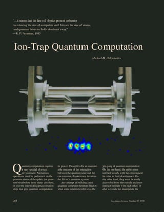
  • 1. “…it seems that the laws of physics present no barrier to reducing the size of computers until bits are the size of atoms, and quantum behavior holds dominant sway.” —R. P. Feynman, 1985 Quantum computation requires a very special physical environment. Numerous operations must be performed on the quantum states of the qubits (or quan- tum bits) before those states decohere, or lose the interlocking phase relation- ships that give quantum computation its power. Thought to be an unavoid- able outcome of the interaction between the quantum state and the environment, decoherence threatens the life of a quantum system. Any attempt at building a real quantum computer therefore leads to what some scientists refer to as the yin-yang of quantum computation: On the one hand, the qubits must interact weakly with the environment in order to limit decoherence. On the other hand, they must be easily accessible from the outside and must interact strongly with each other, or else we could not manipulate the Ion-Trap Quantum Computation Michael H. Holzscheiter 264 Los Alamos Science Number 27 2002
  • 2. quantum state, implement quantum algorithms, and read out the result of a calculation in a timely fashion. How can we hope to meet such con- tradictory goals? Ion-trap quantum computers, as originally proposed by Ignacio Cirac and Peter Zoller (1995), offer a possi- ble solution to this dilemma. As its name implies, an ion trap confines charged particles to a definite region of space with magnetic and electric fields. In a specific realization of such a trap, called a linear radio-frequency quadru- pole (RFQ) trap, or a linear Paul trap (Raizen et al. 1992, Walther 1994), time-varying electric fields are used to hold a line of ions in place—like pearls on a string. These ions serve as the physical qubits of the quantum com- puter. Immobilized by the trapping fields and confined inside an ultrahigh vacuum chamber, they are effectively isolated from the environment. However, by addressing individual ions with sharply defined laser beams, we can initialize the computer, control the qubit states during the operation of logic gates, and read out the results at the end of the computation. The inter- action between the individual ions is mediated by the Coulomb force between the charged particles. This article discusses the design principles for isolating single ions in a linear Paul trap (Paul et al. 1958), whose operational principles are described in detail. The individual ele- ments of an ion-trap computer will be introduced, and how to initialize, manipulate, and interrogate the qubits will be explained. Specific schemes that were implemented in the quantum computation project at Los Alamos (Hughes et al. 1998) will illustrate the descriptions. Ion-trap quantum compu- tation is rapidly evolving, and numer- ous groups around the world are developing new ideas and experimen- tal techniques. The reader will get a flavor of this activity in the last section of the article, which summarizes sev- eral important results achieved within the last few years: the on-demand cre- ation of entangled states of up to four ions by the National Institute of Science and Technology (NIST) group in Boulder, Colorado; the development of a novel cooling scheme by a group at the University of Innsbruck, Austria, which would allow researchers to quickly cool large numbers of trapped ions with drastically reduced opera- tional overhead; and the construction of an effective defense against the forces of decoherence. The Physics of Ion Traps Two basic types of devices can confine charged particles to well- defined regions of free space: Penning traps and Paul traps. The Penning trap, which was primarily developed by Hans Dehmelt at the University of Washington in Seattle, uses a strong magnetic field and a static electric field to create a nearly perfect three- dimensional, harmonic trapping potential (Dehmelt 1967). Some of the most precise tests of fundamental physical symmetries to date have been conducted with this device, whose operating principles are described in the box “The Penning Trap” on the next two pages. Although Penning traps nicely solve the fundamental problems of ion confinement, so far they have not been used for quantum computation. The trap’s strong magnetic field causes ions to move rapidly in a circle (the cyclotron motion dis- cussed in the box), whereas we want the physical qubits to have as little motion as possible. That is why the favored trap for quantum computa- tion is the Paul trap, in which there is no magnetic field and oscillating electric fields (as opposed to static ones) confine the ions. This device was invented by Wolfgang Paul from the University of Bonn in Germany, who shared the 1989 Nobel Prize in physics with Dehmelt. Paul enjoyed telling the following anecdote about how he hit upon the idea for his device. Germans like soft- boiled eggs for breakfast, and on a particular Sunday morning, Paul had prepared two eggs of different sizes and had placed them on a serving tray. When he started to walk, tray in hand, toward the bedroom to surprise his wife with breakfast in bed, the eggs began to roll. He counteracted their motion by shaking the tray and was able to confine the larger egg to the center by shaking with a particular frequency and amplitude. (It was cer- tainly not a well-defined harmonic shaking.) The smaller egg, however, kept rolling toward the edge, so Paul changed amplitude and frequency and successfully prevented this egg from falling, at the expense of allowing the larger one to wobble toward the edge. Whether he ever reached the bedroom with both eggs on the tray and enjoyed a leisurely breakfast with his wife remains unknown, but that morning Paul realized not only the basic princi- ple of the RFQ trap but also the mass- selective feature of such an instrument. At that time, he was keen on develop- ing a mass filter for ions, that is, a two-dimensional structure that could transmit an ion with a specific charge-to-mass ratio and not any other ratio. Eventually, Paul’s idea was used to generate three-dimensional, mass- selective confinement systems, but Cirac and Zoller returned to the origi- nal two-dimensional structure and proposed using it as the basis for a quantum computer. The Linear Paul Trap. To under- stand the linear RFQ trap, consider a positively charged ion floating in free space and surrounded by four infi- nitely long conducting rods, as shown in Figure 1. We can give one pair of opposing rods a positive charge and the other pair a negative charge Number 27 2002 Los Alamos Science 265 Continued on page 268
  • 3. + + + Capacitor plate B-field line + + + Capacitor plate 266 Los Alamos Science Number 27 2002 Ion-Trap Quantum Computation The Penning Trap Decades before individual ions were considered as candidates for qubits in a quantum computer, experimental physicists were challenged to realize a simpler Gedanken, or thought, experiment embodied by the statement often made by theorists: “Consider a single (silver) ion in a uniform magnetic field” (Tanoudji et al. 1977). Thought became reality in 1973, when Hans Dehmelt and his col- leagues at the University of Washington in Seattle were able to capture a single charged particle in a Penning trap. The ion that drifted into the central region of that device was trapped by a strong, uniform magnetic field and by the electro- static field produced by a set of specially shaped electrodes. The entire device operated under ultrahigh vacuum to limit the interactions between the ion and the background atoms. The University of Washington group refined the technique and used the trap to confine a single electron (Wineland et al. 1973) and later a single barium ion, using an RFQ Paul trap (Neuhauser et al. 1980), and performed precision spec- troscopy on these systems. The special arrangement of fields caused the single electron to behave as if it were bound to a nucleus for it displayed a set of energy levels, or excited states, similar to those of the hydrogen atom. Dehmelt therefore named his electron in a Penning trap “geonium—a single electron bound to Earth.” The artificial geonium “atom” was, in a sense, closer to per- fection than a real atom. The spacing between energy levels was nearly con- stant because it reflected the trap’s nearly perfect harmonic-oscillator potential. Dehmelt and coworkers used geonium to perform some of the most precise tests of fundamental symmetries. In a more mundane fashion, Dehmelt called the ion ASTRID (for “a single trapped ion dancing”). (Perhaps, if you keep an ion or electron for such a long time, you may become attached to it.) To understand the operating principles of the Penning trap, consider a charged particle (ion) moving freely in space. To confine it to a specific spot in space, we can apply electrical forces to its charge. If we place the ion between two parallel conducting plates that are charged to an electric potential of the same sign as the ion, the Coulomb repulsion will keep the particle from moving closer to either plate (see Figure A). The ion can still move in directions parallel to the conductors. We can try to remove all escape routes by placing more conductors around the particle. But Michael Faraday discovered more than 150 years ago that an electric field cannot penetrate a closed metal enclosure—hence, the penchant for science museums to place a person inside a “Faraday cage” that is then exposed to violent lightning bolts. The courageous volunteer remains unharmed because the lightning’s electric field vanishes inside the cage. Similarly, if we fully enclose our particle in a cage of conducting plates, the electric field disappears, and we lose the forces holding the particle from the walls. A more successful approach is to use the fact that an electric charge moving in a magnetic field will experience a force perpendicular to the direction of both the magnetic field and the particle’s velocity (the Lorenz force F = qv × B). Therefore, if we apply a magnetic field perpendicular to our parallel conducting plates (see Figure B), we force the ion onto a circular path around the magnetic field line, closing off the sideway escape routes. Figure A. Electrostatic Forces The positively charged particle is repulsed by the capacitor plates but is free to move anywhere in the horizontal plane. Figure B. Applying a Magnetic Field A magnetic field causes the ion to circle around a field line (cyclotron motion), thus confining the ion in the horizontal plane.
  • 4. Whereas the system shown in Figure B can confine charged particles (and has been used for a number of experiments), the special character of the Penning trap is given by the clever shaping and arrangement of the electrodes. As shown in Figure C, two end caps shaped as hyperbolae of revolution replace the paral- lel plates, and a ring-shaped center electrode defines the electrostatic potential on the edge of the trap. The arrangement shown in Figure C not only leads to perfect confinement of individual charged particles but also allows the motion of a trapped particle to be separated into three independent harmonic motions. In order of decreasing frequency, the three motions are (1) the fast “cyclotron” motion of the charge around the magnetic field lines, (2) a slower oscillation in the direction of the magnetic field that is due to the electrostatic repulsion from the two end caps, and (3) a much slower drift motion that is due to the crossed electric and mag- netic fields (see Figure D). The drift motion is easily understood if one focuses on the cyclotron motion. The positively charged particle is accelerated toward the negatively charged ring electrode as it moves away from the electrical center of the trap. This acceleration increases the radius of curvature for the outer half of the cyclotron motion. As the particle moves back toward the center during the second half of the cyclotron motion, it decelerates, and the radius of curvature decreases. The net effect is a distortion of the circular cyclotron motion into a spiral that bends around the electrical center of the trap, as seen in Figure E. The harmonic motions account for the almost constant spacing between energy levels in Dehmelt’s geonium atom, but this orderliness is hardly noticeable in the roller-coaster-like motion of a trapped particle. If you actually want to expe- rience the particle’s motion yourself, there is a carnival ride in which these three components of motion are present—but watch your stomach! Number 27 2002 Los Alamos Science 267 Ion-Trap Quantum Computation Figure D. Motion in the Penning Trap The three-dimensional motion of an ion in the trap consists of three harmonic motions: a fast cyclotron motion, a slower up-down oscillation, and a slow circular drift motion. B E Distorted cyclotron motion E × drift motion + B Axis of symmetry B-field arrow + Trapping region – Figure C. The Penning Trap The two endcaps, which are hyperbolae of revolution, replace the flat capacitor plates. The central ring electrode helps define the harmonic potential at the center of the trap. Figure E. Drift Schematic of the drift motion that results from the crossed electric (E) and magnetic (B) fields.
  • 5. (relative to some arbitrary “zero” potential).1 The positive ion feels a repulsive force from the positively charged conductors and is pushed toward the center of the trap. The ion simultaneously feels an attractive force due to the negatively charged conductors and is pulled outwards. If we now reverse the polarity of our four electrodes, interchanging plus for minus and minus for plus, the ion’s motion will begin to reverse. Where it was moving out, it will now be moving in, and vice versa. However, if the reversal takes place quickly, the “heavy” ion cannot easily respond; it has too much inertia to follow the fast changes in the electric field exactly. Instead, the ion will respond to the time-averaged electric field. If we switch the polarity of the electrodes at a few megahertz (or a few million times a second) by applying a radio-frequency (rf) voltage and if the amplitude is correct, then the time-averaged field generates a harmonic pseudopoten- tial with its minimum located at the trap axis. The ion is pushed to the bottom of the pseudopotential 268 Los Alamos Science Number 27 2002 Ion-Trap Quantum Computation Figure 1. Principles of the Linear Paul Trap (a) The linear Paul trap consists of four conducting rods. Two opposing rods are connected to one pole of a radio- frequency (rf) voltage source, whereas the remaining two are connected to the other pole. The axis of symmetry between the rods is the trap axis. (b) With the rods charged as shown, the resulting electric force pushes a positive ion to the nega- tive rods and repels it from the positive ones. (c) Half an rf period later (see graph below), the polarity of all rods is reversed, and the direction of the force also reverses. (d) If the polarity changes fast enough, a heavy ion becomes stuck in a rapid back-and-forth motion. Because the electric fields are at a minimum at the trap axis, an effective force pushes the ion toward the center, where it becomes trapped (although it is still free to move along the axis). The blue dots seen between the rods in part (a) represent a string of radially trapped ions. The string can be confined axially when a positively charged electrode (end cap) is placed at each end of the rods. rf + + – – rf +/– rf (b) t = t 1 (a) (d) Time Average + + – – rf (c) t = t 2 +/– +/– +/– rf Voltage + – 0 t1 Time rf Voltage + – 0 t2 Time rf Voltage + – 0 Time 1 For reasons discussed on the previous two pages, all four conductors cannot be positively charged, or the electric fields within the trap would disappear. Continued from page 265
  • 6. well and becomes trapped forever— at least in principle—near the center. To generate the mass selectivity sought by Paul, we add a positive direct-current (dc) component to the rf voltage. Positive ions outside a cer- tain mass range feel less of a restoring force from the pseudopotential and are kicked out of the trap by the repul- sive dc field. This technique is one of several that we can use to preferen- tially retain qubit ions instead of, say, a residual gas ion that may be present in the ultrahigh vacuum trap. Of course, the ion’s motion is still unrestricted in the direction parallel to the trap’s axis. For confinement in this third dimension, we simply add an electric dc potential to a pair of “end electrodes” that are on either side of the region of interest. This axial field plugs up the escape route along the symmetry axis of the system, and the ion becomes trapped in three dimensions. By substantially reducing the ion’s energy (cooling), we coax the ion into lying along the central portion of the trap axis, where the radial and axial confining potentials are at a minimum. If several very cold ions are in the trap, then they all fall to the center, and the mutual Coulomb repulsion between the ions causes them to line up neatly along the axis. Motion in the Trap. Although the combination of rf and dc fields within the trap drives the ion into a complex radial motion, that motion is fully described by a set of differential equa- tions called “Mathieu’s Equations.” The bound solutions of those equa- tions yield a stability diagram that allows one to evaluate the effective- ness of the trap, given the values of several critical parameters, such as the amplitudes of the rf and dc compo- nents of the voltage, the rf, the ion mass, and the size of the trap (Dawson 1976). As long as we keep the values of the critical operational parameters within certain ranges, an ion will remain bound to the axis of the device. Furthermore, the magnitude of the restoring force of the pseudopotential holding the ions in the radial direction will remain directly proportional to the distance from the center—the hallmark of a harmonic potential.2 In other words, to a good approxima- tion, the ions will undergo harmonic oscillations in the radial direction with frequency ωr (or with frequency ωx and ωy in case the potential is different in the x- and y-directions). This motion is commonly referred to as the secular motion. The ions’ motion can become dis- torted if the minima of the rf field and the pseudopotential are misaligned within the trap. Misalignment can occur because of some small asymme- try in the trap’s construction or because of small dc patch potentials on the electrode surfaces. Regardless of the reason, misalignment will cause the ions to lie “off center” (that is, off the line where the rf field vanishes). Those ions will experience the strong gradient of the rf field and undergo rapid oscillations—at the frequency of the applied rf field—around their time-averaged equilibrium position. This so-called micromotion is the main source of ion heating. We can suppress the micromotion by adding a compensating dc voltage to some of the rf electrodes (or to auxiliary con- trol electrodes) and thereby shift the ions’ positions closer to the actual rf center. In addition to exhibiting secular motion and the unwanted micromo- tion, an ion or, more important, a string of ions will also vibrate in the axial direction. The motion will be harmonic because the dc voltage on the end electrodes creates a harmonic potential along some length of the trap axis. The vibrations are similar to those exhibited by a set of pendula connected to each other by springs; the swinging of one pendulum sets the others in motion (see Figure 2). Unlike vibrations of classical pendula, however, the vibrations exhibited by a string of ions are quantized; that is, the amplitude of the motion depends on the number of quanta (phonons) in the vibrational mode. For N ions in a trap, there are N axial vibrational modes and an additional 2N modes for motions transverse to the axis. Each mode has a distinct vibrational frequency. The lowest-frequency (lowest-energy) vibration is the so-called common mode, in which the ions oscillate back and forth in unison along the axis. This mode figures heavily in the origi- nal quantum-computing scheme of Cirac and Zoller. Because all ions participate in the common-mode oscillation, when we add (or remove) a quantum of energy to this motion by interacting with one of the ions, we influence all other ions in the string. Any two qubits, regardless of the dis- tance between them, can therefore be coupled together to perform logic operations. Other proposals make use of some of the higher-frequency modes to couple qubits together (James 1998a). These modes have more-complex vibrational patterns and relatively higher excitation energies than the common mode, but it still takes very little energy to excite them. Even a string of very cold ions will vibrate in some intricate expression of the various modes, a problem that is addressed in the discussion of ion cooling. If only a few ions are confined in the trap, the ions will align themselves linearly along the axis. But increasing the number of ions or increasing the dc voltage applied to the end elec- trodes introduces instabilities because Number 27 2002 Los Alamos Science 269 Ion-Trap Quantum Computation 2 To generate a pure harmonic potential, the four electrodes should have hyperbolic cross sections, but in practice we approxi- mate that ideal shape with cylindrical rods.
  • 7. the ions are effectively squeezed closer together. The Coulomb repulsion between neighboring ions becomes stronger than the radial restoring force, and the ions start buckling out into a zigzag pattern. When even more ions are added, the zigzag pattern develops into a com- plex three-dimensional helical struc- ture (Raizen et al. 1992, Walther 1991, 1994). Some of the ions will move away from the axis and will experience the strongest micromotion heating—a situation clearly to be avoided. We have studied this transi- tion from linear to three-dimensional structures in some detail (Enzer et al. 2000) and have quantified the parame- ter space available for quantum computing in a linear RFQ ion trap. Elements of the Ion-Trap Quantum Computer In 1994, inspired by the great suc- cess of ion traps in the field of preci- sion measurements, Cirac and Zoller proposed that the RFQ ion trap had the right characteristics to support the long sequence of precision operations required for quantum computation. A string of ions trapped along the symmetry axis of the trap would be the quantum register of the computer. Each ion could be addressed by tightly focused laser beams, initial- ized to an arbitrary state, manipu- lated, and then probed at the end of a calculation. Most important, the isola- tion from the environment afforded by the trap would allow for long coherence times. One- and Two-Qubit Operations. The logical qubit states |〉 and |〉 of the ion-trap quantum computer must be defined as they always are for any quantum computer. (To stress that the and used to designate the states are notational and have no numerical meaning, we have used a font differ- ent from the one for the numbers 0 and 1.) We simply identify the ion’s electronic ground state with the qubit state |〉 and a long-lived excited state with the qubit state |〉. We also want to apply a unitary transformation to a single qubit, that is, to implement a one-qubit gate, and rotate the qubit in Hilbert space to an arbitrary superposition of the |〉 and |〉 states. (Two-level systems and the rotation of a qubit in Hilbert space are discussed in the article “Quantum Information Processing” on page 2.) To do so, we subject the ion to a laser pulse of a specific amplitude, frequency, and duration. Assuming the ion is in its ground state, the laser pulse will cause the electron wave function of the target ion to evolve to some superposition of the ground and excited states. (We cause the electron to undergo part of a Rabi oscillation.) Illuminating the ion with a so-called π-pulse, for example, will evolve the electron wave function through half a Rabi oscillation period and leave the ion in the excited state. The qubit would have rotated from the |〉 to the |〉 state. If the duration of the pulse is halved (a so-called π/2-pulse), the ion would be left in an equally weighted superposition of the ground and excited states. The qubit would have rotated to the 1/√2(|〉 + |〉) state. 270 Los Alamos Science Number 27 2002 Ion-Trap Quantum Computation Figure 2. Vibrational Modes A set of strongly coupled pendula can be used to envision the vibrational motion of a string of ions in a harmonic potential. These vibrational modes affect all ions simultaneously. If we set any one of the pendula in motion, the others will move. Similarly, if we grab hold of any pendulum and stop it, all others will stop. (a) The common mode (center-of-mass mode), in which all pendula swing one way and then the other, has the lowest frequency (lowest energy) of all modes. Using this mode to couple two qubits together in the trap is the basis of the Cirac-Zoller proposal. (b) The breathing mode, in which pendula at opposite ends move in opposite direc- tions, has the next highest frequency. For an odd number of pendula, the middle one does not move. This mode is less susceptible to heating by external noise sources and has also been used to couple qubits. (c) Shown here is another higher- order mode. In an ion trap, the ions can vibrate in three dimensions; for N trapped ions, there are 3N vibrational modes. (a) Common Mode (b) Breathing Mode (c) Higher-Order Arial Mode
  • 8. While we can use laser pulses to interact with each qubit separately (and excite a qubit’s electronic, or internal, degrees of freedom), we can also use another laser to excite the trap’s vibrational modes and hence to interact with all qubits simultaneously. The latter process can be viewed as interacting with the qubits’ external degrees of freedom. The state of a string of j qubits in the trap is there- fore explicitly given as |q1, q2, … qj〉|n〉 . (1) The first ket, |q1, q2, … qj〉, refers to the logical qubit states, with qj = or . The second ket, |n〉, refers to the common-mode vibrational state, and the value of n, say, 0, 1, 2, …, indi- cates the number of phonons in the common mode. (Although the string of qubits may initially be in another mode, we will restrict our attention to the common mode.) Thus, in the state |q1, q2, … qj〉|0〉 , (2) the ions are not vibrating because there are no phonons in the common mode. In the state |q1, q2, … qj〉|1〉 , (3) the common mode contains one phonon and all the ions are swaying in unison along the trap axis. As mentioned earlier, the common mode is used as a “bus” that couples different ions together. To better understand this coupling, consider first that the frequency of the transi- tion between the |〉 state and the |〉 state is ω0, and that the common- mode vibrational frequency ω1 is much lower than ω0. Similar to the case of two coupled harmonic oscilla- tors, the energy spectrum of the ion exhibits resonances not only at the “carrier” frequency ω0, but also at the “sideband” frequencies ω0 ± ω1 (see Figure 3). The resonance with the higher frequency is commonly known as the blue sideband; the one with the lower frequency, as the red sideband. For cold ions, the linewidth ∆ω0 of the carrier transition is very narrow3 and is less than the energy difference between the carrier and either side- band. Thus, the sidebands and the car- rier can be resolved within the cold ion’s frequency spectrum. Now consider, for example, a pro- cedure used to place two ions in an entangled state. Assuming that the ions are initially in the state |〉|0〉, if we were to address the first ion with a π-pulse from a laser detuned to the blue sideband of the internal tran- sition, both the internal and external states of that ion would be excited. Because an excitation in the common mode is felt by both ions, the result would be the two-qubit state |〉|1〉. If, instead, we address the first qubit Number 27 2002 Los Alamos Science 271 Ion-Trap Quantum Computation Energy n – 1〉 n〉 n + 1〉 Red Blue Carrier Common-mode vibrational states 0 – 1 0 0 + 1 (a) Resolved Sideband Structure Carrier transition Red sideband Blue sideband (b) Resonant Transitions 〉n〉 →〉n – 1〉 〉n〉 →〉n + 1〉 〉n〉 →〉n〉 〉 〉 ω ω ω ω ω Figure 3. Vibrational Sideband Spectrum (a) An ion trap naturally couples an ion’s electronic excitations to its vibrational motion. Each electronic transition at resonant frequency ω0, known as the carrier frequency, is therefore accompanied by other sideband transitions. We show the two side- bands closest in frequency to the carrier: the lower-energy red sideband at frequency (ω0 – ω1), and the higher-energy blue side- band at frequency (ω0 + ω1). A laser with a sufficiently narrow linewidth can interact with the ion via a specific sideband or the carrier. (b) Interacting with a particular qubit (ion) via a sideband transition will change the qubit’s internal state and simultane- ously the external state of all the qubits in the trap, either increasing the number of phonons in the common mode by one (exci- tation on the blue sideband) or decreasing the number by one (excitation on the red sideband). 3 The metastable excited state has a very long lifetime, which leads to a narrow linewidth according to Heisenberg’s uncertainty principle. To take an example from the Los Alamos experiment, a cal- cium ion excited to the 32D3/2 state will decay to the ground state only after an average delay of about 1 second, which results in a transition linewidth of about 1 hertz.
  • 9. with a π/2-pulse (see Figure 4), both qubits are placed in a superposition of the two states, namely, 1/√2(|〉|0〉 + |〉|1〉) . (4) We then address the second ion (which is still in its ground state) with a π-pulse tuned to the red side- band. The laser energy is too low to excite directly the ground-to-excited- state electronic transition, but the transition still occurs if extra energy can be taken from the common mode. The end result is that all phonons have been removed from the quantum register at the end of the operation, and we create a two-qubit entangled state: 1/√2(|〉 + |〉)|0〉 . (5) We can no longer describe the system as individual ions being in the ground or the excited state. The result of a measurement on one ion is strongly correlated to the status of the other ion. Notice that this procedure works equally well if one or more ions are placed in between the first and second ions because the excitation of the common mode is shared by all ions. Besides defining the individual operations just described, Cirac and Zoller also spelled out in detail the steps needed to perform a “controlled- not” (cnot) gate. In such an operation, a “target qubit” flips its state only if a second qubit, the “control qubit,” is originally set to its logical |〉 value. Dave Wineland’s group at NIST first implemented the cnot gate in an ion trap in 1995 (Monroe et al. 1995), albeit using only a single ion in the trap. (The two states of the control qubit were the two lowest-energy trap vibrational states.) Still, because any computation can be performed with a number of two-qubit cnot gates, together with some single-qubit gate operations, the realization of a cnot gate in a quantum computer is an important benchmark. Readout. At the end of any quan- tum calculation, the individual qubits in the quantum register will be in defined states, which must be read out with high fidelity. A powerful readout tool makes use of the phenomenon of quantum jumps (Sauter et al. 1986, Bergquist et al. 1986). The readout method is easily understood when one examines the generic ion-level scheme 272 Los Alamos Science Number 27 2002 Ion-Trap Quantum Computation The vibrational state is indicated by the position of the ions on the rungs of a ladder in the harmonic potential well. In this diagram, the electronic ground state of an ion is indi- cated by a solid circle; the excited state, by an open circle. (a) Suppose two qubits are initialized to the state | 〉|0〉. Addressing the first qubit with a π-pulse from a laser tuned to the blue sideband will excite the ions to the state | 〉|1〉. The first ion is in its electronic excited state, while the second remains in its electronic ground state. Because the common mode affects all ions, both ions are excited to the |n = 1〉 vibrational state. (b) Two qubits can be entangled if we illuminate the first qubit with a π/2-pulse on the blue sideband. The ions are placed in a superposition of states: 1/√2(| 〉|0〉 + | 〉|1〉). If the second ion is then illumi- nated by a π-pulse from a laser tuned to the red sideband, it can absorb the photon only if energy is available from the vibrational mode. Thus, ion 2 is excited only if ion 1 was excited; it remains in the ground state if ion 1 was in the ground state. The two-ion system therefore exhibits the strong correlation of observables, which according to Bohr, define the condition of entanglement. The end result of the operation is the entangled state 1/√2(| 〉 + | 〉)|0〉. n = 1〉 n = 0〉 Internal State Excited:〉 Ground:〉 〉0〉 〉0〉 〉1〉 + + Red sideband π-pulse on 2nd ion Blue sideband π/2-pulse on 1st ion Blue sideband π-pulse on 1st ion (a) Coupling Two Qubits through the Common Mode (b) Entangling Two Qubits √2 (〉0〉 +〉1〉 ) — 1 √2 (〉 + 〉 ) 0〉 — 1 Figure 4. Using the Common Mode to Entangle Two Qubits
  • 10. shown in Figure 5. The ion has two states that we identify as the logical qubit states |〉 and |〉. But the ions used for quantum computation also have a short-lived excited state |s〉 that is accessible from one of the qubit states, the |〉 state, by laser excita- tion. When the laser drives the |〉 — |s〉 transition for a long period, the ion fluoresces and emits a huge number of photons. If that transition is not accessible because the ion was in the |〉 state, there will be no fluores- cence. Detection of a fluorescence signal, therefore, tells us that the qubit is in the |〉 state, and we observe the “jumps” of the ion between the |〉 and the |〉 state as distinct jumps in the intensity of the fluorescence. This type of readout will destroy any quantum information contained in the qubit state and will yield a purely For example, suppose the ion is in an equal superposition of the states |〉 and |〉; then probing the ion once with the laser will not reveal the original state of the qubit. If we want to get a reading on the ratio of the two different states in a superposition, we will have to repeat the measurement multiple times and resort to a statistical description. If we want to maintain the quan- tum character of the ion’s state at the end of a particular calculation, we may resort to a different scheme. Consider an ion placed in a high- quality optical cavity, which is tuned to the resonance of the internal transi- tion in the ion. If the ion is in the state |〉, a photon is emitted into the cavity; if it is in the state |〉, no photon is emitted. If the ion is in a superposi- tion state, the photon field in the cav- ity will end up in a superposition between the states consisting of one photon in the cavity and no photon in the cavity. Thus, the quantum state of an ion or an atom can be transferred to a photon (Parkins and Kimble 1999, Mundt et al. 2002). This state could be transferred through optical fibers to a different trap and then transferred into another ion—and so, the quantum Internet is born! The Los Alamos Ion-Trap Quantum Computing Experiment Currently, every implementation of ion-trap quantum computing uses qubits that are composed of two long- lived internal states of the trapped ions (the ground state and a metastable excited state, or two hyper- fine sublevels of the ground state) and has the qubits communicating with each other through the trap’s vibra- tional modes. Many different ion species can serve as qubits, and numerous qubit schemes are possible. While the previous section discussed ion-trap quantum computers in gen- eral terms, this section describes an experiment developed at Los Alamos, in which calcium ions were used. We initially chose to use calcium for a number of reasons, including the following: All the wavelengths needed for cooling and manipulation are, at least in principle, accessible by rela- tively inexpensive diode lasers; the lifetime of the metastable state allows a reasonable number of coherent operations to be performed; and the calcium isotope of interest is most abundant and can easily be loaded Number 27 2002 Los Alamos Science 273 Ion-Trap Quantum Computation s〉 〉 Qubit transition 〉 Readout transition Figure 5. Readout Using Quantum Jumps (a) A generic three-level scheme for ions in a trap is illustrated. The qubit states | 〉 and | 〉 are typically the ground state and a long-lived excited state, respectively. The state |s〉 is short lived and is coupled to the ground state. If the ion is in the ground state, a laser can drive the | 〉 → |s〉 transition many times per second, and the ion will fluoresce. If the ion “jumps” to the | 〉 state, there will be no fluorescence, so that the presence or absence of a large fluorescence signal reveals the state of the qubit. (Alternatively, one can use two long-lived ground-state hyperfine levels as qubits and construct a similar readout scheme.) (b) This composite image shows strings of calcium ions that were laser-cooled to near rest in the Los Alamos quan- tum computation ion trap. The spacing between the ions is approximately 30 µm. About 108 photons are absorbed and reemitted each second during the time the readout laser is irradiating the ion. That photon flux is easily detectable with a charge-coupled device (CCD) camera. The fluorescence is actually bright enough to be seen with the naked eye, except that for calcium, the readout transition is at 397 nm and is outside the range of sensitivity for the human eye. (a) Generic Three-Level System (b)
  • 11. into the trap. But the basic quantum computational schemes outlined earlier can be implemented with any element that displays an ionic-level structure similar to that of calcium, such as the other alkali-earth elements beryllium, magnesium, strontium, and barium. At this stage of experimenta- tion, all alkali-earth ions are essen- tially interchangeable, and for mostly technical reasons, calcium has recently been replaced with strontium in our quantum computing experi- ment. (Some of that work is described in the article, “Quantum Information with Trapped Strontium Ions” on page 178.) In addition, other ions, such as mercury and ytterbium, also exhibit level schemes that are applicable to quantum computation, albeit with slightly different technical approaches. As ion-trap quantum computers become more sophisti- cated, the choice of ion species will become a larger issue. Our trap is a linear Paul trap, about 1 centimeter in length and 1.7 mil- limeters in diameter, with a cylindrical geometry, as seen in Figure 6(a). We create the strong, radial confine- ment fields by applying a few hundred volts of rf amplitude at approximately 8 megahertz to two opposing rods. The remaining two rods are rf-grounded. The axial confinement, which prevents the ion from leaking out of the trap along the symmetry axis, is produced by a direct current of about 10 volts applied to each of the conical end caps. This combination of the rf and dc fields leads to an axial oscillation frequency ω1 for the com- mon mode of a few hundred kilohertz and a radial oscillation frequency of ωr ≈ 1 megahertz. Additional dc potentials can be applied to four support rods, which are not shown in Figure 6(a) but are located outside the actual trap elec- trodes. In this way, one can center the ion string on the electrical sym- metry axis of the trap and thus mini- mize the amount of heating produced by micromotion. Figure 6(b) shows a schematic diagram of the internal-level structure of calcium ions and gives the wave- lengths of the relevant transitions. (Any other alkali-like ion would have a similar structure.) The 42S1/2 ground state and the metastable 32D5/2 excited state are used to form the logical qubit states |〉 and |〉, respectively. The metastable excited state has a lifetime of about 1 second, which is long enough to allow an interesting number of computational steps to be per- formed before decoherence (resulting from spontaneous emission from the excited state) can destroy the internal state of the quantum register. To load the ions into the trap, we cross a beam of calcium atoms that is produced by heating a small calcium- filled reservoir with a beam of elec- trons emitted by an “electron gun.” (The electron gun is essentially identi- cal to the one inside a computer moni- tor or a television screen.) These two beams are aligned so that they cross each other within the effective volume of the trap, that is, within the cylindri- cal volume that fits between the four rods and the two end caps. The atoms 274 Los Alamos Science Number 27 2002 Ion-Trap Quantum Computation Figure 6. The Los Alamos Linear Paul Trap (a) The trap built at Los Alamos for quantum computation is about 1 cm in length and 1.7 mm in diameter. An electric field of a few hundred volts oscillating at 8 MHz is applied to two of the conducting rods. The other two rods are RF grounded. About 10 V of a direct current is placed on the conical end caps. (b) This illustration shows a partial energy-level diagram for calcium (not to scale) and shows the wave- lengths of some transitions relevant to our quantum computing scheme. The qubit transition is shown in red. 42 P 3/2 42 P 1/2 42 S 1/2 393 nm 397 nm 729 nm 866 nm 854 nm  〉 32 D 5/2 τ = 1.14 s 32 D 3/2 τ = 1.16 s  〉 (b) Partial Energy-Level Diagram for Calcium Conical endcap Conducting rod (a) Trap Built at Los Alamos
  • 12. that are ionized by electron impact suddenly feel the confining forces of the electric fields and become trapped. Cirac and Zoller (1995), as well as other authors, proposed initializing the computer in the state | … 〉|0〉 ; (6) that is, all qubits are in their electronic and vibrational ground states. However, the temperature4 of the newly trapped ions is very high, since their energy is given by a combination of the temperature of the calcium oven and the energy imparted to the ion by the electric field. (The latter energy varies, depending on where the ionization occurs.) In order to reach the initial state and then to perform quantum logic operations, the ions’ temperature must be reduced to its lowest possible value. Cooling the ions takes place in two steps described in the next two sections. Doppler Cooling of Calcium Ions. As its name suggests, this first cool- ing step makes use of the Doppler effect, whereby the relative motion between a source and an observer causes a change in the observed fre- quency of an acoustic or electromag- netic wave. For example, the sound of a siren on an ambulance or a police car changes its pitch depending on whether the vehicle moves toward you or away from you. Similarly, an ion or atom will absorb or emit photons of different frequencies (energies), depending on its motion relative to the light source. Although an ion in the trap is localized by elec- tric fields and its average velocity is zero, the variation of the instanta- neous velocity, as the ion jiggles back and forth due to thermal motion, causes the inherent emission and/or absorption profile of an ionic transi- tion to become much broader than the natural linewidth of the transition (second-order Doppler broadening). For “hot” ions, the Doppler-broad- ened linewidth is typically much greater than the laser linewidth. To implement Doppler cooling, we tune a laser to a frequency below the resonance frequency of a transition in the ion (Figure 7). Only when it is moving at a certain velocity toward the laser can the ion absorb these “off-resonance” photons, because only then does it “see” the laser frequency shift into resonance. However, as a result of its random jiggling, the ion has a probability to emit photons at any frequency within its Doppler- broadened emission line profile. One can easily see from Figure 7 that the ion has a greater probability to emit a photon with a higher frequency than the absorbed photon. On average, Number 27 2002 Los Alamos Science 275 Ion-Trap Quantum Computation Ion at rest “sees” frequency . Doppler-broadened emission profile Ion moving into the laser with velocity v “sees” frequency + = (1 + v/c). Ion moving out of the laser with velocity v “sees” frequency – = (1 – v/c). (a) Frequency Shifts Due to the Doppler Effect Laser Ion (b) Detuning (c) Doppler Cooling of Calcium E = h E0 Energy Laser line 42 P1/2 42 S1/2 〉 32 D3/2 τ = 1.16 s 〉 m 866 nm 397 nm ω ω ω ω ω ω Figure 7. Doppler Cooling of Ions (a) When interacting with a laser of frequency ω, an ion at rest sees the native laser frequency. If the ion is moving, this frequency is shifted by the Doppler effect. An ion moving into the laser beam “sees” the laser frequency Doppler-shifted toward a higher frequency, ω+, while the ion moving in the direction of the laser beam “sees” the frequency ω–. (b) This first-order Doppler effect is eliminated in ion traps because the average velocity is zero. However, because of its thermal motion, the ion has a probability to absorb photons at any frequency within its Doppler-broadened absorp- tion profile. Similarly, it has a probability to emit a photon over a range of frequen- cies within its emission profile. Suppose the laser is tuned below the ion’s resonance frequency ω0 so that ω ω0. When the ion moves into the laser beam, it will absorb a photon because it sees the laser frequency Doppler-shifted close to its resonance frequency (ω+ ∼ ω0). The ion absorbs a laser photon of energy E = h hω h hω0, but on average it reemits a photon with higher energy (from the gray region). Because it loses energy during each cycle of absorption and emission, the ion cools rapidly to the limit of this method, which is imposed by the recoil energy the ion experiences upon reemission of the photon. For typical parameters of our trap, calcium will reach a vibrational level of approximately |n = 10〉 to |n = 30〉 at the end of the Doppler cooling. (c) The transitions used to Doppler-cool calcium ions are shown. 4 We often refer to ion temperature rather than energy because the ions show a distribution of energies over time.
  • 13. more energy is emitted than absorbed, which leads to a cooling of the ion. For rapid cooling, a large number of photons must be absorbed and emitted, and therefore Doppler cool- ing is performed on a transition that can be cycled rapidly. We use the 397-nanometer transition from the 42S1/2 to the 42P1/2 state. The lifetime of the 42P1/2 state is about 10 nanoseconds, so the ion can absorb and reemit about 108 photons per second. Unfortunately, the 42P1/2 state has a chance of roughly 1 in 15 to decay into the metastable 32D3/2 state, which has a lifetime of about 1 sec- ond. The ion then takes so long to return to the ground state that it would be lost from the cooling cycle. To avoid this outcome and force ions to return from the D3/2 level to the cool- ing cycle, we irradiate the ion with two lasers: the cooling laser at 397 nanometers and a “repump” laser at 866 nanometers. Doppler cooling has its limits. Conservation of momentum guaran- tees that, after emitting a photon in one direction, the ion recoils in the opposite direction. Although this recoil energy is small, eventually it counteracts any cooling effects. For calcium ions, the Doppler limit is equivalent to a temperature of about 3 microkelvins. At that temperature, the kinetic energy of the ions is signif- icantly less than the mutual Coulomb repulsion between ions. Essentially, they do not have enough kinetic energy to leap-frog each other, so the cold ions remain frozen in their rela- tive locations and form a string. The photos in Figure 4 are examples of ion strings that were realized in our trap. At a 200-kilohertz common-mode frequency, the spacing between ions is about 30 micrometers. Even at a temperature of 3 microkelvins, however, the ions have enough energy to occupy any of several vibrational modes, with many phonons per mode. (The specific dis- tribution of states depends on the ions’ temperature and the frequency of each mode.) Here, we will restrict our attention to the common mode. After Doppler cooling, the ions in the trap can typically occupy the states from |n = 10〉 to about |n = 30〉. Getting the qubits into the common-mode ground state (|n = 0〉), therefore, requires an additional cooling scheme. Sideband Cooling of Calcium. We recall that ions in the trap can couple their internal degrees of free- dom with their external motion, which leads to sidebands at ω0 ± ω1, where ω1 is the common-mode frequency, in the absorption spectrum. For cold ions with a minimal Doppler linewidth, these sidebands are resolvable from the carrier—see Figure 8(b). Thus, an ion can absorb photons not only at the carrier frequency ω0 of their internal |〉 → |〉 transition but also on the upper and lower sidebands at the frequencies ω0 ± ω1. Assuming all ions are in the state |〉|n〉, we can tune a laser with a suitably narrow linewidth to the red sideband— photon energy [E– = h(ω0 – ω1]—and excite one of the ions to the state |〉|n – 1〉. In essence, energy is removed from the vibrational mode (the occupa- tion number is reduced by one phonon) and is used to make up the deficit in photon energy. After its radiative life- time, the ion can decay to one of three states: the state |〉|n – 2〉, by emitting a photon with energy [E+ = h(ω0 + ω1]; the state |〉|n – 1〉, by emitting a photon with energy [E0 = hω0]; or a return to its initial state, by emitting a photon with energy [E– = h(ω0 – ω1]—see Figure 8(c). On average, the ion loses one vibrational photon of energy E = hω1 for each excitation–decay cycle. Because we started somewhere around |n = 30〉, we need about 30 cycles to bring the vibrational mode to its ground state(provided there are no competing effects that heat the ions while they are being cooled). Unfortunately, the long lifetime of the 32D5/2 state is now a hindrance. In principle, we can scatter only one photon per second using this transi- tion, which would render the process of cooling from |n = 30〉 to |n = 1〉 unacceptably slow. Heating processes —micromotion heating or simply radiative heating from other noise sources in the system—are much faster, and we would be unable to reach the desired starting point of all qubits being in the internal and external ground states. To speed things up, we artificially shorten the lifetime of the 32D5/2 state by introducing an alternate decay route via the 42P3/2 state (Marzoli et al. 1994). We irradiate the ion not only with a laser tuned to 729 nanometers (to drive the S–D transition), but also with a second laser tuned to 854 nanometers—see Figure 8(d). The second laser pumps the ion from the D- to the P-state, from which the ion rapidly returns to the ground state. By carefully choosing the amplitude of the 854-nanometer laser, we can design the effective lifetime of the 32D5/2 state according to our needs, and our calcium ion can jump down the ladder of harmonic-oscillator levels in just 3 to 30 milliseconds. In a real system, the cooling power from the lasers will always be in com- petition with external heating processes. Although no clear theoreti- cal explanation of these processes has emerged, many possibilities have been discussed in the literature, and the rele- vant scaling laws with trap parameters have been developed (James 1998b). Typical candidates—besides micromo- tion heating, which can be avoided by carefully tuning the trap voltages—are fluctuating contact potentials on the trap electrodes (originating from insu- lating deposits on the electrodes), which have a frequency component at the trap’s resonant frequency. In the absence of a proper theoreti- cal description of ion heating, we can 276 Los Alamos Science Number 27 2002 Ion-Trap Quantum Computation
  • 14. turn to empirical data accumulated from a number of different experi- ments. The adopted procedure is to cool the ions to as low a temperature as possible and then turn off the lasers responsible for the cooling. After a variable delay time, we measure the ion’s temperature using sideband spectroscopy. Quentin Turchette and coworkers (2000) conducted the most complete study of this type when they looked at heating effects in traps of different sizes. The separate traps had also undergone different preparation “rituals.” The studies suggest a strong dependence on trap size, that is, on the distance between the ions and the trap electrodes. When the studies are combined with observations made by Rainer Blatt’s group at the University of Insbruck, one is led to believe that “bigger is better.” But Ralph deVoe with IBM has recently reported that hardly any heating was observed over a short period in a miniaturized trap. Clearly, we have much to learn before we can understand the heating of ions in rf traps. The comforting thought is that, in all cases, the time scale for heating from the ion’s ground state can be kept long, com- pared with the time required for a reasonable number of quantum manipulations. Furthermore, heating times are typically longer than times for other decoherence processes. Readout of the Calcium Ion. We use the |s〉 = 42P1/2 excited state in calcium for readout, the same state that is used for Doppler cooling. As discussed earlier, this state has a life- time of only 10 nanoseconds and is accessed from the ground state by a laser tuned to 397 nanometers. An ion in the |〉 state will absorb and reemit about 108 photons per second when the laser drives the |〉 → |s〉 transition. (Because the 42P1/2 state can also decay to the long-lived 32D3/2 state, we simultaneously irradiate the ion with a laser tuned to Number 27 2002 Los Alamos Science 277 Ion-Trap Quantum Computation Figure 8. Sideband Cooling (a) This partial energy-level diagram shows the transitions we use for sideband cooling of calcium ions. (b) When the linewidth of the carrier transition (frequency ω0) is very narrow and the Doppler broadening is minimal, the ion’s vibrational side- bands can be resolved. (c) The figure shows several vibrational levels for the | 〉 → | 〉 carrier transition. If a single ion is initially in the state | 〉|n〉, then illuminat- ing the ion with a laser tuned to the red sideband will excite the ion to the state | 〉|n – 1〉. The latter state will decay to | 〉|n – 2〉 or | 〉|n – 1〉, or it will go back to | 〉|n〉. On average, the number of phonons in the mode decreases by 1 after each excita- tion/emission. (d) The lifetime of the upper level may be artificially shortened if that level is coupled to an auxiliary one with a higher decay rate. The faster decay will increase the cooling rate. 1 0 1 D D D D D S S S S n – 3 – 〉 n – 2 – 〉 n – 1 – 〉 n〉 n n – 3 – 〉 n – 2 – 〉 n – 1 – 〉 n〉 n D D D S S S S P P P P 〉 〉 〉 〉 Sideband cooling nm 854 n 32 D5/2 42 P3/2 42 S1/2 393 nm 0 29 nm = 72 (a) Sideband Cooling Transitions (c) Stepping to Lower Vibrational States (d) Increasing the Cooling Rate (b) Resolved Sideband Structure 〉 〉 ω0 ω ω ω ω ω ω1 ω 0 ω ω
  • 15. 866 nanometers to return the ion to the 42P1/2 state.) Even with a modest photon-collection efficiency of about 10–4, which is due to experimental considerations (we cannot bring a lens too close to the ions without blocking access to the trap), we can easily detect the photons scattering from the ion with a charge-coupled device (CCD) camera. In Figure 9, we show a sample trace of the detected photon counts for a sin- gle ion in the trap. The fluorescence signal is nominally about 104 counts per second. We randomly excite the ion with a laser tuned to 729 nanome- ters, and each time it “jumps” from the |〉 state to the |〉 state, the signal dis- appears. Figure 9 also shows the fluo- rescence from a set of two ions. The different levels of intensity are for both ions being excited (no fluorescence), for one of the two ions being excited (intermediate fluorescence), and finally, for both ions being in the ground state (full fluorescence). Although it is easy to distinguish among these cases, determining which of the two ions is in the ground state for the intermediate fluorescence level is difficult. We must look at the ions individually, by focusing the laser on one ion at a time, and then convert to the single-ion measurement. Ferdinand Schmidt-Kaler and his colleagues from the Innsbruck group have used this readout technique with three ions, which were spaced at about 6 micrometers from each other in the trap. They cooled the ions to the |〉|n〉 state, and all three were emitting photons on the readout tran- sition. The scientists then pointed a sharply focused laser at 729 nanome- ters onto one of the ions and placed it in the |〉 state (the dark state). The measured crosstalk among neighbor- ing ions was less than 1 percent, so the state of the chosen qubit could be determined with about 99 percent fidelity (Nägerl et al. 1999). Important Developments A Popular Mechanics article from 1949 stated, “Where a calculator on the ENIAC (electronic numerical integrator and calculator) is equipped with 18,000 vacuum tubes and weighs 30 tons, computers in the future may have only 1000 tubes and weigh only one and a half tons.” That observation did not turn out to be entirely correct. How could anyone have foreseen the development of transistors and integrated solid-state circuitry or the remarkable parallel developments that have culminated in today’s supercomputers? We are still in the “vacuum-tube” era of quantum computation, and if asked two years ago about the future of ion-trap-based quantum computers, 278 Los Alamos Science Number 27 2002 Ion-Trap Quantum Computation Quantum Jumps, Single Ion Calcium Readout Transitions Time (s) 0 Fluorescence (counts/s) 6000 4000 2000 0 Quantum Jumps, Two Ions Fluorescence (counts/s) 14000 8000 2000 0 12009 10000 6000 5 10 15 〉 〉 〉 〉 or 〉 〉 4000 Time (s) 0 5 10 15 (a) (b) (c) 729 nm 〉 32 D5/2 32 D3/2 s〉 42 P1/2 42 S1/2 〉 397 nm 866 nm Figure 9. Readout of Qubits (a) Shown here are the readout transitions for calcium. (b) For this readout experi- ment, a single ion interacts with two lasers: a low-intensity laser that drives the qubit transition | 〉 → | 〉 and a second laser that drives the readout transition | 〉 → |s〉. The fluorescence signal from that transition, nominally around 4,000 counts per second, is recorded with a simple rate meter. When the qubit is in the | 〉 state, we can drive the readout transition, but if the ion occupies the state | 〉, the fluorescence disappears. We can distinguish between the | 〉 and | 〉 states with nearly 100% fidelity. (c) The state of two ions can also be distinguished. No count corresponds to the state | 〉; 8000 to 10,000 counts per second correspond to the state | , 〉; 4000 counts per second, to either | 〉 or | 〉. (In the last case, our experi- mental setup does not allow us to distinguish between the two states.)
  • 16. I would have been hesitant to promise much. I may have argued that the systems we were looking at were mere demonstrations, designed to help us understand the fundamental physics issues behind qubits and that the prospects for scaling these devices up to a larger number of qubits were doubtful. Even today I could argue that, while the computing scheme of Cirac and Zoller is in principle scala- ble (Hughes et al. 1996), it has yet to be realized with two qubits. However, because much has hap- pened in the ensuing two years, included here are descriptions of just a few of the many important develop- ments that have put the ion-trap quantum computer back on the track for scalable technologies. Similar to the transition from vacuum tubes to solid-state devices (even if not quite as fundamental), these developments do not invalidate any of the previous achievements and underlying princi- ples but are unpredicted and significant enhancements of available technology. Four-State Entanglement. To take full advantage of the power of quantum computation, we need to generate entanglement between an arbitrary number of qubits. But generating any entangled state is dif- ficult. In the case of photons, entan- glement is achieved by means of a statistical process. Many pairs of pho- tons are created by a method known as parametric down-conversion, whereby a high-energy photon, after entering a special type of crystal, has a certain probability to convert into two photons, each with half the initial energy. In a few cases, two photons emerge in an entangled state. (See the article “Quantum State Entanglement” on page 52.) We can typically produce about 1000 entan- gled pairs per second, but if we look for entanglement of three or even four photons, the likelihood of finding such a state becomes unacceptably small for practical purposes (30 per second for 3 photons and a few per year for four photons). Thus, quantum computing took a leap forward when the NIST team in Boulder demonstrated that it could produce an entangled state of up to four ions “on demand” (Sackett et al. 2000). Based on a proposal by Anders Mølmer and Klaus Sørenson (1999) from the University of Aarhus in Denmark, the NIST team around Chris Monroe and David Wineland demonstrated the feasibility of entan- glement of two and four ions in a deterministic way. With a single-pulse operation of two lasers, the desired state could be produced with a high degree of certainty. To understand the technique, con- sider two spin-half particles confined in a harmonic well and coupled by vibrational degrees of freedom. (The spin description is equivalent to our previous picture of two internal states in an ion.) The NIST group used the two ground-state hyperfine levels of 9Be+ ions as an effective spin-half system, with |↓〉 = |F = 2, mF = –2〉 and |↑〉 = |F = 1, mF = –1〉. The energy levels of the system are shown in Figure 10, where hω0 is the internal energy splitting of each particle and ν is the oscillation frequency of the par- ticular collective mode of the particles in the trap. The group used standard laser- cooling and optical-pumping tech- niques to prepare the particles in their spin-down internal state and in the ground state of their collective motion: |Ψ〉 = |↓↓〉|0〉. Laser pulses at ω0 + (ν – δ) and ω0 – (ν – δ), where δ is the detuning from the resonance (refer to Figure 10), then drive the two-step transition from |↓↓〉|0〉 to |↑↑〉|0〉. If the detuning δ is sufficiently large, the intermediate states |↑↓〉|〉 Number 27 2002 Los Alamos Science 279 Ion-Trap Quantum Computation Figure 10. Four-Particle Entanglement The figure shows the relevant energy levels and transition frequencies used to cre- ate deterministic multiparticle entanglement. A two-ion scheme is illustrated. The |↑↑〉|0〉 excited state has an energy of 2E0 = 2h hω0. The |↑↓〉|1〉 and |↓↑〉|1〉 excited states, in which the internal state of one of the ions is excited and both ions go into a vibrational excited state, has an energy E1 = h h(ω0 + ν). Lasers tuned to energies E1 + δ and E1 – δ, where δ is a predetermined laser detuning, can directly excite the ions to the |↑↑〉|0〉 state. Pulsing the two lasers for a time t = π/(2Ω), where Ω is an effective Rabi frequency, will place the ions in the entangled state |Ψ2〉 = 1/√2(|↑↑〉 – i|↓↓〉). The scheme can be generalized to any number of ions and has been used to create entangled states of up to four ions. (Figure reproduced with permission from Nature.) h h h 0 h 0 Laser 1 Laser 2 ↑↑〉0〉 ↑↓〉0〉 ↓↓〉0〉 ↑↓〉2〉 ↑↓〉1〉 ↓↑〉0〉 ↓↑〉2〉 ↓↑〉1〉 ω ω δ ν
  • 17. and |↓↑〉|〉 are negligibly occupied, and no motional excitation occurs in the process. Applying the laser fields for a time t = π/(2Ω), where Ω is the Rabi oscillation frequency for the transition, results in the final wave function |Ψ2〉 = 1/√2 (|↑↑〉 – i |↓↓〉) , (7) which is the desired maximally entangled state. It turns out that this process is entirely scalable for an even number of N qubits and can generate the N-particle entangled state |ΨN〉 = 1/√2 × (|↑↑...↑〉–iN+1|↓↓...↓〉) . (8) If N is an odd number, the state |ΨN〉 can still be produced, provided one rotates each qubit independently. The NIST scientists have used this method with two and four ions in the trap, but they also caution that the experimentally realized states |Ψ2〉 and |Ψ4〉 are not fully entangled. Each state shows some degree of decoher- ence. Although the amount of deco- herence in |Ψ4〉 was more than what could be tolerated for quantum com- puting, the achievement of reliably creating a four-particle entangled state on demand cannot be underestimated. In a later development, the NIST group showed that the maximally entangled states of a pair of trapped 9Be+ ions could be used as a decoher- ence-free subspace for protecting one qubit of information against dephas- ing errors (Kielpinski et al. 2001). The decoherence-free subspace, also called a noiseless subsystem, is spanned by the two orthogonal states |Ψ+〉 = 1/√2 (|↓↑〉 + i |↑↓〉) , and |Ψ–〉 = 1/√2 ( |↓↑〉 – i |↑↓〉) . (9) These states serve as the logical qubit for storing information. It is easy to see that all superpositions of these maximally entangled states are invari- ant under transformations that apply the phase change |↑〉 → eiς|↑〉 simulta- neously to both ions. This so-called collective dephasing is thought to be a major source of decoherence for trapped ions. In the NIST experiment, an arbitrary state of one qubit was encoded in the decoherence-free subspace of two ions: α|↑〉 + β|↓〉 → α|Ψ+〉 + β|Ψ–〉 .(10) The encoded information was sub- jected to engineered dephasing errors or ambient errors, and then the encod- ing procedure was reversed to recover the original information. The data showed unequivocally that the noise- less subsystem protects the informa- tion from collective dephasing errors for a time up to ten times longer than the typical decoherence time and that collective dephasing is indeed a major source of errors in ion traps. One could imagine that this type of robust storage might enable the operation of a quantum computer constructed from an array of ion traps as opposed to a single trap. (For an introduction to the theory of noiseless subsystems, see the article “Introduction to Quantum Error Correction” on page 188. A nuclear magnetic resonance experi- ment demonstrating noiseless subsys- tems is presented in the article “Realizing a Noiseless Subsystem in an NMR Quantum Information Processor” on page 260.) Broadband Cooling. The second important recent result is the selective enhancement of the probability of cooling ions by electromagnetically induced transparency (EIT). The scheme of Cirac and Zoller has the qubits coupled together by means of the common vibrational mode, in which all ions oscillate back and forth in unison along the trap axis. However, even two trapped ions have an extra degree of freedom in the axial motion, namely, the breathing mode, in which ions on opposite sides of the string move 180° out of phase (refer to Figure 2). Each additional ion opens up three more vibrational modes to the ion string. Every mode of frequency ν can be assigned an average quantum number nν. The initial scheme of Cirac and Zoller requires a mode to have nν = 0 in order to be used for computational operations. For small numbers of ions, we reach this state by the standard sideband-cooling methods discussed earlier. As seen in Figure 11(a), the ion has a number of transition possi- bilities: Excitation on the lower side- band will cool the ion, excitation on the upper sideband will cause heating, and transitions on the carrier will cause diffusion. In sideband cooling, we use an ultranarrow laser and excite only the lower sideband so that |n〉 → |n – 1〉. For a large number of qubits, how- ever, the sheer number of higher modes makes it technically difficult, if not impossible, to use standard sideband-cooling methods. Not only would we have to identify and excite the lower-sideband transitions for each and every mode, but the spec- trum becomes so “dense” that the upper sidebands of a neighboring internal transition can overlap the lower sidebands of another. Cooling one mode could actually heat another. Furthermore, the “overhead” needed to control and cool these modes is daunting: large numbers of laser pulses, constant retuning of the lasers from one mode to the next, and tight control of the qubit register through- out the cooling stage. For efficient (and simultaneous) cooling of more than one mode, broadband cooling would be required, even though that would seemingly exacerbate the problem of unwanted excitation. But recent work by Blatt’s group at the University of Innsbruck 280 Los Alamos Science Number 27 2002 Ion-Trap Quantum Computation
  • 18. may make broadband cooling possible (Morigi et al. 2000, Roos et al. 2000). The group adopted the EIT technique to selectively enhance the probability of exciting cooling transitions rather than heating transitions in the ion. The necessary asymmetry between lower and higher sidebands can be achieved as follows: Consider a three- level system with two lower levels and one shared excited state—see Figure 11(b). Using a strong coupling laser between one of the ground states and the upper state creates so-called light shifts (that is, shifted energy lev- els, as seen by another probe laser). For a detuning of the coupling laser above the resonance, a probe laser sees an absorption profile that shows zero absorption for a detuning equal to the coupling laser, the so-called Fano profile—see Figure 11(c). Therefore, such a probe would be transparent for that exact detuning— the EIT phenomenon. In order to obtain optimum cooling using these EIT resonances, the detunings are chosen such that the carrier transition is exactly located at the EIT resonance (that is, it is not excited at all because of that quantum interference), and the maximum absorption is chosen to be around the lower sideband frequency. Because the absorption profile generated in this manner is fairly wide (much wider than the natural width of the transition used for tradi- tional sideband cooling), the asym- metry between heating and cooling transitions exists for many modes. Several different modes can be cooled simultaneously with a single operation. This technique reduces the overhead for laser-cooling of multi-ion strings and also eases the requirements for laser stability, which are very strict for standard sideband cooling. To show that EIT cooling can simultaneously cool vibrational modes with significantly different fre- quencies of oscillation, the Innsbruck group chose to cool the axial mode and the radial mode of a single ion confined in a three-dimensional Paul trap at 3.3 megahertz and 1.6 mega- hertz, respectively (Schmidt-Kaler et al. 2001). In a linear trap, the nearby modes (“spectator” modes) are not used for the computation directly; they are coupled to and may affect the common mode. The group achieved ground-state populations of 73 per- cent for the axial and 58 percent for the radial mode. Although this result is certainly not as satisfactory as that achieved by sideband cooling (because of the smaller absorption asymmetries), it is certainly sufficient for cooling (and thus suppressing) those modes. The EIT method promises the possibility of cooling all spectator modes of a multiqubit quantum register with a single operation. That would allow the more elaborate (individual) sideband cooling scheme to be used on only the mode needed for calculations. Outlook Many systems have been proposed in the last several years as potential candidates for becoming quantum computers, including laser-cooled trapped ions (Cirac and Zoller 1995), Number 27 2002 Los Alamos Science 281 Ion-Trap Quantum Computation 〉m – 1〉 〉m –1〉 〉m〉 〉m〉 〉m + 1〉 〉m + 1〉  〉  〉 r 〉 -2 -1 0 1 2 Cooling laser absorption (a.u.) m〉 m – 1〉  m 〉  m + 1〉  k〉  k + 1〉  m 〉  m 〉  k〉  k〉 Relative detuning of the two lasers Coupling laser Probe laser  k〉  k – 1〉 (a) Broadband Excitation (b) EIT Scheme (c) Sideband cooling of a multi-ion string that is accessing many excited vibrational modes is very difficult in that the sideband structure becomes dense and complicated. EIT cooling permits broadband cooling of several vibrational modes, |m〉, |k〉, ... , simultaneously. (a) When a broadband probe laser is applied to the | 〉|m〉 → | 〉|m〉 transition, both cooling (red) and heating (blue) transitions can occur. (b) When a second coupling laser excites the |r〉 → | 〉 transition, the ion’s absorption profile becomes modified. Proper choice of laser detuning (to the dashed state) suppresses heating transitions. This result is evident in figure (c), where the solid line gives the absorption profile for the EIT scheme. For proper tuning of the lasers, the absorption strength for the transition |m〉 → |m〉 is zero and a strong asymmetry between |m〉 → |m + 1〉 and |m〉 → |m – 1〉 transitions is introduced. This asymmetry in absorption between the blue and the red sideband also holds for higher-frequency vibrational modes (|k〉 → |k ± 1〉), allowing simultaneous cooling of several different modes with one broadband laser. [Figure was adapted from Schmidt-Kaler (2001) with permission from the authors.] Figure 11. EIT Cooling
  • 19. nuclear magnetic resonance (Gershenfeld and Chuang 1997, Cory et al. 1998), cavity quantum electro- dynamics (Ye et al. 1999), and more recently, superconducting devices, quantum dots, and silicon-based solid- state devices. From the preliminary experiments performed by several groups world- wide, it is apparent that the existing ion traps are adequate to hold and manipulate small numbers of qubits. Although five to ten qubits hardly a computer make, these numbers are large enough to make the technology well worth pursuing. Ion traps will be a potent tool for exploring, for exam- ple, the possibility of creating entan- gled states of large numbers of qubits. Investigations of the type described here will help us identify the relevant physics issues that must be addressed to achieve computational gains. We should also expect that many of the technologies now being pursued for quantum computation will be super- seded by even more promising ideas. One such idea is to scale up to a larger number of qubits by multiplexing sev- eral ion traps with a specific trap that contains a few qubits acting as the cen- tral processor. After implementing part of a quantum algorithm, the qubits would be shuffled into one of several storage traps, thus allowing new qubits to be loaded into the processor. Recent work also suggests that we could transfer the internal quantum states of a string of ions in a trap to a set of photons in a high-finesse cavity. The quantum information could then be transferred through optical fibers into a second cavity and fed back into an ion string in a different trap. Developments like this will surely continue to happen and will allow us to explore quantum computation well beyond the current state of the art. As we get closer to realizing a small quantum processor, the “time scales” of a particular system become more relevant. In general, the hierar- chy of time scales present in an ion- trap quantum computer is very prom- ising. Manipulations on quantum registers can be done in microseconds, while disturbances by the environment have been shown to be avoidable for milliseconds. The inherent deco- herence time of the quantum state is longer still, for it is limited by the lifetime of the upper qubit state, which is about 1 second in calcium. The decoherence time can be increased even more by an appropriate choice of ions (for example, ytterbium) or by stable ground-state hyperfine levels used as logical qubit states. It is important to point out that despite the revolutionary advances in computers during the last 50 years, the fundamental principle of computa- tion has not changed. Today’s fastest supercomputer operates according to the same rules as the ENIAC. Quantum computation, however, rep- resents a paradigm shift in informa- tion processing. Although a future quantum computer may not look any- thing like our current ion trap, the experience and knowledge we gain now will be of fundamental impor- tance to our understanding this new paradigm of computing. For some researchers, building a quantum computer to break secure codes is an important, and certainly challenging, goal. But for me and most of my colleagues, performing experi- ments that Erwin Schrödinger and Albert Einstein only dreamed of and thus gaining a deep understanding of this “inconceivable” quantum world are far larger rewards. Perhaps we will encounter some failure of conventional quantum mechanics, or perhaps the problems of decoherence will forever keep the quantum realm out of our classical grasp. In any event, the future will be exciting for both quantum physics and computation. Acknowledgments The work described in this article is the result of a close and fruitful col- laboration among numerous experi- mental scientists over several years. I wish to thank them all for their help in the laboratory, as well as for the many intellectual discussions that helped me understand in depth the fundamental principles involved. Over the years, I enjoyed working with Daphna Enzer, John Gomez, Mark Gulley, Paul Kwiat, Steve Lamoreaux, Glen Peterson, Vern Sandberg, Martin Schauer, Dale Tupa, and Justin Torgerson on developing capabilities for quantum computation with trapped ions. In addition, I had the privilege to travel to many groups pursuing this dream and learned much of what I know today about the ion-trap quantum processor from many interactions with my friends and colleagues Rainer Blatt, Ferdinand Schmidt-Kaler, Dietrich Leibfried, Christoph Nägerl, and many others at the University of Innsbruck in Austria; with Andrew Steane, David Lucas, and Derek Stacey from the Clarendon Laboratory in Oxford, the United Kingdom; and last but not least, with all the members in Dave Wineland’s group at NIST, in Boulder (too numerous to name here individually), who took me on challenging excur- sions into the quantum world of trapped ions, as well as into the all too classical world of mountain biking. Further Reading Bergquist, J. C., R. G. Hulet, W. M. Itano, and D. J. Wineland. 1986. Observation of Quantum Jumps in a Single Atom. Phys. Rev. Lett. 57: 1699. Cirac, J. I., and P. Zoller. 1995. Quantum Computations with Cold Trapped Ions. Phys. Rev. Lett. 74: 4091. Cory, D. G., M. D. Price, and T. F. Havel. 1998. Nuclear Magnetic Resonance Spectroscopy: An Experimentally Accessible Paradigm for Quantum Computing. Physica D 120 (1–2): 82. 282 Los Alamos Science Number 27 2002 Ion-Trap Quantum Computation
  • 20. Dawson, P. H., ed. 1976. Quadrupole Mass Spectrometry and Its Applications. Chaps. II and III. Amsterdam: Elsevier Scientific Publishing Co. Dehmelt;, H. G. 1967. Radiofrequency Spectroscopy of Stored Ions, Part I. Adv. At. Mol. Phys. 3: 53. ———. 1969. Radiofrequency Spectroscopy of Stored Ions, Part II. Adv. At. Mol. Phys. 5: 109. ———. 1981. Coherent Spectroscopy on Single Atomic System at Rest in Free Space 2. J. Phys. (Paris) 42: 299. ———. 1988. A Single Atomic Particle Forever Floating at Rest in Free Space: New Value for Electron Radius. Physica Scripta. T22: 102. Enzer, D. G., M. M. Schauer, J. J. Gomez, M. S. Gulley, M. H. Holzscheiter, P. G. Kwiat et al. 2000. Observation of Power-Law Scaling for Phase Transitions in Linear Trapped Ion Crystals. Phys. Rev. Lett. 85 (12): 2466. Gershenfeld, N. A., and I. L Chuang. 1997. Bulk Spin-Resonance Quantum Computation. Science 275: 350. Huang, X.-P., J. J. Bollinger, T. B. Mitchell, and W. M. Itano. 1998. Phase-Locked Rotation of Crystallized Non-Neutral Plasmas by Rotating Electric Fields. Phys. Rev. Lett. 80: 73. Hughes, R. J., D. F. V. James, E. H. Knill, R. Laflamme, and G. F. Petschek. 1996. Decoherence Bounds on a Quantum Computation with Trapped Ions. Phys. Rev. Lett. 77: 3240. Hughes, R. J., D. F. V. James, J. J. Gomez, M. S. Gulley, M. H. Holzscheiter, P. G. Kwiat, et al. 1998. The Los Alamos Trapped Ion Quantum Computer Experiment. Fortschr. Phys. 46 (4–5): 329. James, D. F. V. 1998a. Quantum Dynamics of Cold Trapped Ions with Application to Quantum Computation. Appl. Phys. B 66 (2): 181. ———. 1998b. Theory of Heating of the Quantum Ground State of Trapped Ions. Pys. Rev. Lett. 81: 317. Kielpinski, D., V. Meyer, M. A. Rowe, C. A. Sackett, W. M. Itano, C. Monroe, and D. J. Wineland. 2001. A Decoherence-Free Quantum Memory Using Trapped Ions. Science 291: 1013. Marzoli, I., J. I. Cirac, R. Blatt, and P. Zoller. 1994. Laser Cooling of Trapped Three- Level Ions: Designing Two-Level Systems for Sideband Cooling. Phys. Rev. A 49: 2771. Mølmer, K., and A. Sørensen. 1999. Multiparticle Entanglement of Hot Trapped Ions. Phys. Rev. Lett. 82 (9): 1835. Monroe, C., D. M. Meekhof, B. E. King, W. M. Itano, and D. J. Wineland. 1995. Demonstration of a Fundamental Quantum Logic Gate. Phys. Rev. Lett. 75: 4714. Morigi, G., J. Eschner, and C. H. Keitel. 2000. Ground State Laser Cooling Using Electromagnetically Induced Transparency. Phys. Rev. Lett. 85 (21): 4458. Mundt, A. B., A. Kreuter, C. Becher, D. Leibfried, J. Eschner, F. Schmidt-Kaler, and R. Blatt. 2002. Coupling a Single Atomic Quantum Bit to a High Finesse Optical Cavity. http://eprints.lanl.gov. quant- ph/0202112. Nägerl, H. C., D. Liebfried, H. Rhode, G. Thalhammer, J. Eschnerr, F. Schmidt- Kalerr, and R. Blatt. 1999. Laser Addressing of Individual Ions in a Linear Ion Trap. Phys. Rev. A 60 (1): 145. Neuhauser, W., M. Hohenstatt, P. E. Toschek, and H. Dehmelt. 1980. Localized Visible Ba+ Mono-Ion Oscillator. Phys. Rev. A 22: 1137. Parkins, A. S., and H. J. Kimble. 1999. Quantum State Transfer between Motion and Light. J. Opt. B, Quantum Semiclassical Opt. 1 (4): 496. Paul, W., H. P. Reinhard, U. von Zahn. 1958. Electrical Mass Filters as Mass Spectrometers and Isotope Filters. Z. Phys. 152: 143. Raizen, M. G., J. M. Gilligan, J. C. Bergquist, W. M. Itano, and D. J. Wineland. 1992. Ionic Crystals in a Linear Paul Trap. Phys. Rev. A 45: 6493. Roos, C. F., D. Leibfried, A. Mundt, F. Schmidt-Kaler, J. Eschner, and R. Blatt. 2000. Experimental Demonstration of Ground State Laser Cooling with Electromagnetically Induced Transparency. Phys. Rev. Lett. 85 (26): 5547. Sackett, C. A., D. Kielpinski, B. E. King, C. Langer, V. Meyer, C. J. Myatt, et al. 2000. Experimental Entanglement of Four Particles. Nature 404: 256. Sauter, Th., W. Neuhauser, R. Blatt, and P. E. Toschek. 1986. Observation of Quantum Jumps. Phys. Rev. Lett. 57: 1696. Schmidt-Kaler, F., J. Eschner, G. Morigi, C. F. Roos, D. Liebfried, A. Mundt, and R. Blatt. 2001. Laser Cooling with Electromagnetically Induced Transparency: Application to Trapped Samples of Ions or Neutral Atoms. Appl. Phys. B 73 (8): 807. Steane, A., C. F. Roos, D. Stevens, A. Mundt, D. Leibfried, F. Schmidt-Kaler, and R. Blatt. 2000. Speed of Ion-Trap Quantum-Information Processors. Phys. Rev. A 62: 042305. Tanoudji, C. C., B. Diu, and F. Laloe. 1977. Quantum Mechanics, Vol. I, Chap. IV. B. 3a, p. 403. New York: John Wiley and Sons. Turchette, Q. A., D. Kielpinski, B. E. King, D. Leibfried, D. M. Meekhof, C. J. Myatt, et al. 2000. Heating of Trapped Ions from the Quantum Ground State. Phys. Rev. A 61: 063418. Walther, H. 1991. In Light Induced Kinetic Effects on Atoms, Ions, and Molecules, p. 261. Edited by L. Moi et al. (Pisa, Italy: ETS Editrice). ———. 1994. Atoms in Cavities and Traps. Adv. At. Mol. Opt. Phys. 32: 379. Wineland, D., P. Ekstrom, and H. Dehmelt. 1973. Monoelectron Oscillator. Phys. Rev. Lett. 31: 1279. Ye, J., D. W. Vernooy, and H. J. Kimble. 1999. Trapping of Single Atoms in Cavity QED. Phys. Rev. Lett. 83 (24): 4987. Number 27 2002 Los Alamos Science 283 Ion-Trap Quantum Computation Michael Holzscheiter received his M.S. and Ph.D. degrees in physics from the University of Mainz in Germany, where he studied electrons trapped in Penning traps. As a postdoctoral researcher at Texas AM University, Michael used trapped ions to study collisional processes of astrophysical rel- evance. Later, as an assistant pro- fessor at Texas AM, he participated in a col- laboration with Los Alamos National Laboratory on trapping antiprotons. In 1986, he joined Los Alamos and pioneered the dynamic trapping of high-energy particles in Penning traps. He became principal investigator of the Los Alamos antiproton experiment, which was installed at CERN in 1992. On the basis of his technique’s success, he formed an international collaboration, ATHENA, to create antihydrogen atoms at rest for ultrahigh precision studies of the symmetries between matter and antimatter and served as spokesman for this collaboration from 1995 through 1999. Back in Los Alamos, Michael applied his expertise in ion traps toward a Los Alamos trapped-ion quantum computer, for which he designed the radio-frequency quadrupole trap and helped build and operate the first-generation experi- ment until the fall of 2001. His research interest continues in the application of the ion-trap technology to a wide variety of physics problems.