1. The document discusses effective material properties of fiber reinforced composites using micromechanics. It relates volume averaged stresses and strains in a representative volume element (RVE) to determine effective composite properties. 2. It presents equations for volume fractions and density of constituents using a "rule of mixtures" approach. Maximum theoretical fiber volume fractions are calculated for ideal square and triangular fiber arrays. 3. Elementary mechanics of materials models are used to predict longitudinal modulus, transverse modulus, Poisson's ratio and shear modulus of a fiber reinforced lamina. The models assume perfect bonding and uniform stresses/strains between fibers and matrix.

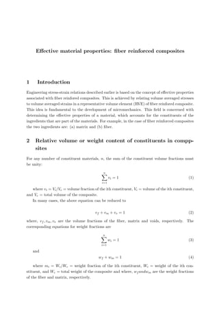
1. Effective material properties: fiber reinforced composites
1 Introduction
Engineering stress-strain relations described earlier is based on the concept of effective properties
associated with fiber reinfored composites. This is achieved by relating volume averaged stresses
to volume averaged strains in a representative volume element (RVE) of fiber reinfored composite.
This idea is fundamental to the development of micromechanics. This field is concerned with
determining the effective properties of a material, which accounts for the constituents of the
ingredients that are part of the materials. For example, in the case of fiber reinforced composites
the two ingredients are: (a) matrix and (b) fiber.
2 Relative volume or weight content of constituents in compp-
sites
For any number of constituent materials, n, the sum of the constituent volume fractions must
be unity:
n
i=1
vi = 1 (1)
where vi = Vi/Vc = volume fraction of the ith constituent, Vi = volume of the ith constituent,
and Vc = total volume of the composite.
In many cases, the above equation can be reduced to
vf + vm + vv = 1 (2)
where, vf , vm, vv are the volume fractions of the fiber, matrix and voids, respectively. The
corresponding equations for weight fractions are
n
i=1
wi = 1 (3)
and
wf + wm = 1 (4)
where mi = Wi/Wc = weight fraction of the ith constituent, Wi = weight of the ith con-
stituent, and Wc = total weight of the composite and where, wf andwm are the weight fractions
of the fiber and matrix, respectively.

2. Figure 1: Representative area elements for idealized square and traingular fiber-packing geome-
tries.
By substituting the product of density and volume for weight in each term above and solving
for the composite density, we get the rule of mixtures:
ρc =
n
i=1
ρivi (5)
or
ρc = rhof vf + rhomvm (6)
where rhoi, ρf , ρm, andρc are the densities of the ith constituent, fiber, matrix and composites,
respectively. The above equations can be rearranged as below
ρc =
1
n
i=1
wi
ρi
(7)
and
ρc =
1
wf
ρf
+ wm
ρm
(8)
The avove equation can also be rearranged so that we get the void volume fraction as
vv = 1 −
(Wf /ρf ) + (Wc − Wf )/ρm
Wc/ρc
(9)
Typical autoclave-cured composites may have void fractions in the range 0.1 − 1%. Without
vaccum bagging, however, volatiles trapped in the composite during cure cycle can cause void
contents of the order of 5%.
Consider representative are elements for idealized fiber packing geometries such as square
and triangular arrays as shown in Fig. 1. It is assumed that fibers are oriented perpendicular
to the page, that the fiber center-to-center spacing ’s’ and the fiber diameter ’d’ do not change
along the length and that the area fractions are equal to the volume fractions. Measurement of
area fractions is possible from photomicrographs and image analysis software.The fiber volume
fraction for the square array is found by dividing the area of fiber enclosed in the shaded square
by the total area of the shaded square:
2

3. vf =
π
4
d
s
2
(10)
The maximum theoretical fiber volume fraction occurs when s = d. In this case,
vfmax =
pi
4
(11)
A similar calculation for the triangular array shows that
vf =
π
2
√
3
d
s
2
(12)
and when s = d, the maximum fiber volume fraction is
vfmax =
π
2
√
3
(13)
In practice, it is not possible to achieve the above close packing configuration of the fibers
to achieve such high volume fractions. Fiber volume fractions, in general, vary from 0.5 to 0.8.
3 Elementary mechanics of materials models
The objective of this section is to present elementary mechanics of materials models for pre-
dicting four independent effective moduli of an orthotropic continuous fiber-reinforced lamina.
In the elementary mechanics of materials approach to micromechanical modeling, fiber-packing
geometry is not specified, so that the RVE may be a generic composite block consisting of fiber
material bonded to matrix material, as shown in Fig. 2. The constituent volume fractions in the
RVE are assumed to be the same as those in the actual composite. Since it assumed that the
fibers remain parallel and that the dimensions do not change along the length of the element,
the area fractions, must equal the volume fractions. Perfect bonding at the interface is assumed,
so that no slip occurs between fiber and matrix materials. The fiber and matrix materials are
assumed to be linearly elastic and homogeneous. The matrix is assumed to be isotropic, but
the fiber can be either isotropic or orthotropic. Following the concept of RVE, the lamina is
assumed to be macroscopically homogeneous, linear elastic and orthotropic. Volume averaged
stresses and strains are used in this elementary approach.
3.1 Longitudinal modulus
In Fig. 2b the RVE is subjected to a longitudinal normal stress, σc1. The response is governed by
the effective longitudinal modulus, E1. Static equilibrium requires that the total resultant force
on the element must be equal to the sum of forces acting on the fiber and matrix. Combining
the static equilibrium condition with average stress we get the following form
σc1A1 = σf1Af + σm1Am (14)
where subscripts c,f, and m refer to composite, fiber and matrix, respectively, and the second
subscript refers to the direction. Since area fractions are equal to the corresponding volume
3

4. Figure 2: RVE and simple stress states used in elementary mechanics of materials models. (a)
Representative volume element, (b) longitudinal normal stress, (c) transverse normal stress, and
(d) in-plane shear stress.
4

5. Figure 3: Variation of composite moduli with fiber volume fraction (a) predicted E1 and E2
from elementary mechanics of materials models and (b) comparison of predicted and measured
E1 for E-glass/polyester.
fractions, the above equation can be rearranged to give the rule of mixture for longitudinal
stress as,
σc1 = σf1vf + σm1vm (15)
Under the assumptions that the matrix is isotropic, that the fiber is orthotropic, and that
all materials follow 1D Hooke’s law, we get
σc1 = E1εc1 σf1 = Ef1εf1 σm1 = Emεm1 (16)
Hence, the rule of mixture of stress equation becomes,
E1εc1 = Ef1εf1vf + Emεm1vm (17)
Note: If fiber and matrix is assumed to be isotropic then we can drop the secod subscript 1
as modulus in 1 and two direction will be same.
The key assumption, due to perfect bonding is that the average displacements and strain in
the composite, fibe and matrix along the 1 direction is same, thus we have
E1 = Ef1vf + Emvm (18)
This equation predicts a linear variation of the longitudinal modulus with fiber volume fraction,
as shown in Fig. 3.
Validity of the key assumption can be assessed by following the strain energy approach. Under
the given state of stress the total strain energy stored in the composite, Uc can be represented
as the sum of the strain energy stored in fibers Uf and the strain energy in the matrix Um.
Uc = Uf + Um (19)
5

6. The total strain energy can be written in terms of average stress-strain relation as below
Uc =
1
2 Vǫ
σc1εc1dV =
1
2
E1ε2
c1Vc (20)
Uf =
1
2 Vf
σf1εf1dV =
1
2
Ef1ε2
f1Vf (21)
Um =
1
2 Vm
σm1εm1dV =
1
2
Em1ε2
m1Vm (22)
Again, if we assume that strain are equal then we get the rule of mixtures. What happens
if the assumption of equal strain is not made? Let the stresses in the fibers and the matrix be
defined in terms of the composite stress as follows:
σf1 = a1σc1 σm1 = b1σc1 (23)
where, a1andb1 are constants. Substitution of the above equation in the rule of mixtures for
stress gives us
a1vf + b1vm = 1 (24)
Using this in the equation of strain energy terms leads to
1
E1
= a2
1
vf
E2
f1
+ b2
1
vm
E2
m1
(25)
Note that we did not assume equal strains to derive the above equation. However, from
experiments on E-glass/epoxy it was found that the values of a1andb1 were such that it leads to
the fact that strain are equal in fiber, matrix and the composite.
3.2 Transverse modulus
If the RVE in Fig. 2c is subjected to a transverse normal stress σc2, the response is governed by
the effective transversemodulus E2. Geometric compatibility requires that the total transverse
composite displacement δc2 must be equal to the sum of the corresponding displacements in the
fiber δf2 and the matrix δm2
δc2 = δf2 + δm2 (26)
It follows from the definition of normal strain that
δc2 = εc2L2 δf2 = εf2Lf δm2 = εm2Lm (27)
Since the dimensions of the RVE do not change along the 1 direction, the length fractions
must be equal to the volume fractions, and the above equations take the form to get the rule of
mixtures for strain as
εc2 = εf2vf + εm2vm (28)
The 1D Hooke’s laws for this case is
σc2 = E2εc2 σf2 = Ef2εf2 σm2 = Emεm2 (29)
6

7. Note: The Poisson strain have been neglected.
Using the above constitutive relation in the rule of mixture of strains we get
σc2/E2 = (σf2/Ef2)vf + (σm2/Em2)vm (30)
If we now assume the stresses in the composite, matrix, and the fiber are all equal then we
get the inverse rule of mixtures for the transverse modulus as
1
E2
=
vf
Ef2
+
vm
Em2
(31)
As in the case of longitudinal case, the strain energy approach provides additional insight
into the micromechanics of the transverse loading case. We now express the fiber and matrix
strains in terms of the composite strain as
εf2 = a2εc2 εm2 = b2εc2 (32)
where a2andb2 are constants. Substitution into the compatibility expression leads to
a2vf + b2vm = 1 (33)
Substituting this into the strain energy expression using the constitutive relation leads to the
general form
E2 = a2
2Ef2vf + b2
2Em2vm (34)
Experiments on E-glass/epoxy showed that the values of a2 and b2 did not lead to situation where
the stresses were same in the composite, matrix and fiber. Hence, in general, this assumption
leading to the derivation of inverse rule of mixture is not valid. However, inverse rule of mixture
does give an easy way to determine E2 in a quick way.
3.3 Poisson ratio and Shear modulus
The major Poisson’s ratio, ν12, and the in-plane shear modulus, G12, are most often used as the
two remaining independent elastic constants for the orthotropic lamina. The major Poisson’s
ratio, which is defined as
ν12 = −
εc2
εc1
(35)
when the only non-zero stress is a normal stress along the 1-direction, can be found by solving
the geometric compatibility relationships associated with both 1 and the 2 directions. The result
is another rule of mixtures formula
ν12 = νf12vf + νmvm (36)
The effective in-plane shear modulus is defined as
G12 =
σc12
γc12
(37)
where σc12, γc12 are the average shear stress and strain, respectively. An equation for the
in-plane shear modulus can be derived using an approach similar to that which was used for the
7

8. Figure 4: Division of RVE into subregions based on square fiber having equivalent fiber volume
fraction.
transverse modulus. That is, geometric compatibility of the shear deformations, along with the
assumption of equal shear stresses in fibers and matrix, leads to another inverse rule of mixtures:
1
G12
=
vf
Gf12
+
vm
Gm
(38)
Note: E1, nu12 determined here are sufficiently accurate for design purpose. However, E2
and G12 are not accurate enough but gives a good first estimation of the material constants.
3.4 Improved mechanics of materials models
A square array of fibers is shown in Fig. ??. The RVE is divided into subregions for more
detailed analysis if we convert to a square fiber having the same area as the round fiber. The
equivalent square shown in Fig. ?? must then have the dimension
sf =
π
4
d (39)
and from the geometry we can also infer the size of the RVE to be
s =
π
4vf
d (40)
The RVE is divided into subregions A and B. In order to find the effective transverse modulus
for the RVE, we first subject the series arrangement of fiber and matrix in subregion B to
a transverse normal stress. Following the procedure described earlier, the effective transverse
modulus for this subregion, EB2, is found to be
1
EB2
=
1
Ef2
sf
s
+
1
Em2
sm
s
(41)
where the matrix dimension is sm = s − sf . It can also be see that
sf
s
=
√
vf
sm
s
= 1 −
√
vf (42)
Hence, EB2 now takes the form
EB2 =
Em2
1 −
√
vf (1 − Em2/Ef2)
(43)
8

9. The parallel combination of subregions A and B is now loaded by a transverse normal stress and
the procedure described earlier is followed to find the effective transverse modulus of the RVE.
The result is rule of mixture given by
E2 = EB2
sf
s
+ Em
sm
s
(44)
The above expression leads to the form
E2 = Em (1 −
√
vf ) +
√
vf
(1 −
√
vf )(1 − Em2/Ef2)
(45)
A similar result maybe found for G12. Note that here expressions have derived in the general
form assuming properties of fiber and matrix are different along 1 and 2 direction, respectively. If
fiber properties are same in 1 and 2 direction then Ef1 = Ef2 = Ef and if the matrix properites
are same in 1 and 2 direction then Em1 = Em2 = Em.
3.5 Effective properties of thermal and moisture coefficients
Following the procedure used in determining the effective longitudinal modulus and by using
the 1D Hooke’s law given below for a lamina subjected to thermo-mechanical loading along with
exposure to moisture
{ε} = [S] {σ} + {α} ∆T + {β}c (46)
The above expression can be expanded and written in matrix form as below:
Figure 5: Hygrothermal constitutive relation for a lamina
Note: Thermal coefficients and moisture coefficient transform like strains.
The effective thermal and mositure coefficients are determined just like before and they are
given below:
α1 =
Ef1αf1vf + Em1αm1vm
Ef1vf + Em1vm
(47)
α2 = αf2vf + αm2vm (48)
β1 =
Ef1βf1vf + Em1βm1vm
Ef1vf + Em1vm
(49)
β2 = βf2vf + βm2vm (50)
9