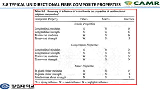
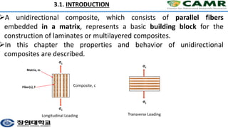
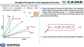
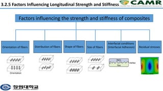
1) The document discusses the behavior and properties of unidirectional composites, which consist of parallel fibers embedded in a matrix. It describes methods for predicting the longitudinal and transverse stiffness and strength of these composites. 2) The rule of mixtures is presented as a way to calculate the longitudinal stiffness and strength of a composite based on the properties of its constituents and their volume fractions. Factors that influence the longitudinal properties are also discussed. 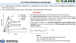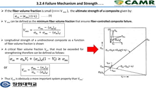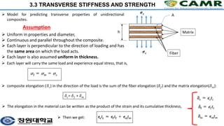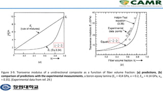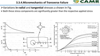3) Transverse properties are generally much lower than longitudinal properties due to the orientation of the fibers. Methods for predicting transverse stiffness using elasticity principles are described. Failure modes in composites include fiber breaking and matrix microcracking.

1. Course Title: Smart Materials Engineering
[SMB2003-00]
CHAPTER THREE: Behavior of Unidirectional Composites
March 2023
Reference: Analysis and Performance of Fiber Composites, Agarwal, B.D.

2. 3.1. INTRODUCTION
A unidirectional composite, which consists of parallel fibers
embedded in a matrix, represents a basic building block for the
construction of laminates or multilayered composites.
In this chapter the properties and behavior of unidirectional
composites are described.
Matrix, m
Fiber(s), f
σc
σc
σc
σc
Transverse Loading
Longitudinal Loading
Composite, c

3. 3.2 Nomenclature
A unidirectional composite is shown schematically in Fig. 3-1.
Several unidirectional layers can be stacked in a specified sequence of
orientation to fabricate a laminate that will meet design strength and stiffness
requirements.
(a) unidirectional lamina (b) multidirectional laminate
Fig. 3-1
A simple layer, ply, or lamina Laminate

4.  shows different properties in the longitudinal and transverse directions.
are orthotropic with the axes x1, x2, and x3 as the axes of symmetry (Fig. 3-1).
Strongest properties in the longitudinal direction.
material behavior in the other two directions (x2, x3) is
nearly identical.
or ply can be considered to be transversely isotropic;
that is, it is isotropic in the x2-x3 plane.
A unidirectional composite

5. 3.2. Volume and Weight Fractions
Factors determining the properties of composites is the relative proportions of
 matrix and
 reinforcing materials.
 Consider a volume vc of a composite material that consists of volume vf of the fibers and volume vm of the
matrix material.
𝒗c = 𝒗𝒇 + 𝒗𝒎 𝑉𝑚=
𝒗𝒎
𝒗𝒄
𝑉𝑓=
𝒗𝒇
𝒗𝒄

6. To establish conversion relations between the weight fractions and the volume fractions, the
density ρc of the composite material must be obtained.
 By similar manipulations, the density of composite materials in terms of weight fractions can
easily be obtained as

7. Now the conversion between the weight fraction and volume fraction ca be obtained by
considering the definition of weight fraction and replacing I it the weights by the products of
density and volume as follows:
The inverse relations are;
&
&
A composite material with only
two constituents

8. For an arbitrary number of constituents. The generalized equations are:
Theoretical density ≠ experimentally determined density. Due to voids in the composite.
Volume fraction of voids Vv:
 In an actual composite, the void content may be determined by following ASTM (American Society for Testing and Materials)
Standard D2734-94 (reapproved 2003).
Where: Vv = the volume fraction of voids
𝜌𝑐𝑡 = the theoretical composite density
𝜌𝑐𝑒 = the experimentally determined composite density

9. Initial Stiffness
 A unidirectional composite may be modeled by assuming fibers to be uniform in properties and diameter,
continuous, and parallel throughout the composite (Fig. 3-3).
 It may be further assumed that a perfect bonding exists between the fibers and the matrix so that no slippage
can occur at the interface, and the strains experienced by the fiber, matrix, and composite are equal:
ϵf = ϵm = ϵc
 For this model, the load Pc carried by the
composite is shared between the fibers
Pf and the matrix Pm so that
Pc = Pf + Pm
 The loads Pc, Pf, and Pm carried by the composite, the fibers, and the matrix, respectively, may be written as
follows in terms of stresses σc, σf , and σm experienced by them and their corresponding cross-sectional areas Ac,
Af, and Am. Thus
Pc = σc Ac = σfAf+ σmAm
Or
σc= σf
𝐀𝐟
𝐀𝐜
+ σm
𝐀𝐦
𝐀𝐜
Model for predicting longitudinal behavior of unidirectional composites

10. Initial Stiffness …
But for composites with parallel fibers, the ,volume fractions are equal to the area ,fractions
such that:
Vf=
𝐀𝐟
𝐀𝐜
Vm=
𝐀𝒎
𝐀𝐜
 Thus,
σc= σfVf+ σmVm
 Now this Eq. can be differentiated with respect to strain, which is the same for the composite, the fibers, and the matrix.
 The differentiation yields
𝐝σc
dϵ
=
𝐝σ𝒇
dϵ
Vf +
𝐝σ𝒎
dϵ
Vm
 Where (
dσ
dϵ
) represents the slope of the corresponding stress-strain diagrams at the
given strain.
 If the stress-strain curves of the materials are linear, the slopes (
dσ
dϵ) are constants and can be replaced by the corresponding
elastic modulus in Eq. (2). Thus
Ec = EfVf+EmVm
. . . . . . . . . . . . . (1)
. . . . . . . . . . . . . (2)
. . . . . . . . . . . . . (3)

11. Initial Stiffness
 Equations (1)-(3) indicate that the contributions of the fibers and the matrix to the average composite properties are
proportional to their volume fractions. Such a relationship is called the rule of mixtures.
 Equations (1) and (3) can be generalized as
σc =
𝒊=𝟏
𝒏
σ𝒊 Vi Ec =
𝒊=𝟏
𝒏
E𝒊 Vi
Example 3-1: Calculate the ratios of longitudinal modulus of the composite to the matrix modulus for glass-epoxy and
carbon-epoxy composites with 10% and 50% fibers by volume. Elastic moduli of glass fibers, carbon fibers, and epoxy resin are
70, 350, and 3.5 GPa, respectively.
Equation (3) can be written as
Solution:
Ec
Em
=
𝐄𝐟
𝐄𝐦
− 𝟏 𝐕𝐟+1
System (Ef/Em)
Ec/Em
Vf = 10% Vm =50%
Glass-epoxy (20) 2.9 10.5
Carbon-epoxy (100) 10.9 50.5
Calculations will give the following results:
 It may be observed that as the fiber volume
fraction increases by a factor of 5, the ratio of 𝐄
𝐜/𝐄𝐦also increases by a similar factor (3.62 for
glass epoxy and 4.63 for carbon-epoxy).

12. Equilibrium of forces: Applied force is shared by the matrix and fiber:
Matrix, m
Fiber(s), f
Fc
Fc
Composite, c
L
δL
Geometry of Deformation: Total strain in the composite will be the same as
in the fibers or the matrix.
. . . (1)
. . . (2)
. . . (3)
The Stress-strain relationships will be given as;
. . . (4a,b,c)
3.2.2 Load Sharing

13. Combining (2) and (4a,b,c) and applying F = σA, where A is the cross sectional area of the specimen,
. . . (5)
Now applying equation (3), we can write
. . . (6)
If the fibers extend to the full length of the composite, then the area ratio will be the same as the volume ratio (=Volume
fraction). We can write,
. . . (7)
Equation (7) is also Known as the Rule of Mixture.
Similarly relations can also be written to determine strength, Poisson’s ratio, thermal conductivity etc in the fiber direction.
Rule of Mixture

14. Strength of Composite in the longitudinal Direction
 We can write Equation (4.2b) in the form of Force=Stress X Area as,
Dividing both sides by
. . . (8)
we obtain
. . . (9)
 Again, the surface ratios can be replaced with volume ratios for longitudinal fiber composites and we can write,
. . . (10)
Strength of the composite
 Now, for calculating the ultimate strength of the composite, we replace the stresses to the maximum possible stress which is
the ultimate tensile strength of the composite, the fiber and the matrix. Therefore,
. . . (11)
Ultimate Strength of the composite
 If Vf and Vm are known

15. Strength of Composite in the longitudinal Direction
 Schematic Stress-strain behavior of the fiber,
matrix and composites in different fiber
orientation arrangements
Fiber
Matrix
00
900
450
Best Strength
Poor Strength
 Since at the point of fracture of brittle fibers, the composite
will fail which means the matrix will be stresses only up to the
fracture strain of the fiber. Hence, should be replaced by
which is the stress in the matrix at the strain equal to the
fracture strain of the fibers.
 Lower value but more realistic ultimate strength of composite.
. . . (12)

16. Rule of Mixture is Applicability
 It is found that the Rule of mixture is applicable for Strength calculation is only applicable if the volume fraction
of fibers is above a critical value.
 This critical value is defined by the following formula (at the critical
point the two lines cross each other):
 From the figure, we can see that the effect of strengthening is effective only
above V1. The value V1is obtained as follows:
. . . (13)
. . . (14)
. . . (15)
 The maximum volume of fiber fraction that can be achieved is ~ 0.8
 Actual strength that can be achieved is ~65% of the theoretical value.
NB:

17. 3.2.3 Behavior beyond Initial Deformation
The rule of mixtures accurately predicts the stress-strain behavior of a unidirectional
composite subjected to longitudinal loads, provided that Eq. (1) is used for the stress and Eq.
(2) for the slope of the stress-strain curve.
However, the simplification of Eq. (2) to Eq. (3) through the replacement of slopes by the
elastic moduli is possible only when both the constituents deform elastically.
This may constitute only a small portion of the composite stress-strain behavior and is
applicable primarily for glass or ceramic-fiber-reinforced thermosetting plastics.
In general, the deformation of a composite may proceed in four stages [l], summarized as
follows:
1. Both the fibers and the matrix deform in a linear elastic fashion.
2. The fibers continue to deform elastically, but the matrix now deforms nonlinearly/plastically.
3. The fibers and the matrix both deform nonlinearly or plastically.
4. The fibers fracture followed by the composite fracture.

18. 3.2.5 Factors Influencing Longitudinal Strength and Stiffness
Factors influencing the strength and stiffness of composites
Orientation of fibers Distribution of fibers Size of fibers
Interfacial conditions
(Interfacial Adhesion) Residual stresses
Shape of fibers

19. 3.2.4 Failure Mechanism and Strength
 In a unidirectional composite subjected to a longitudinal load, failure initiates when the fibers are strained to
their fracture strain.
 This assumes that the failure strain of the fibers is less than that of the matrix.
 For theoretical predictions, that all the fibers fail at the same strain.
 If the fiber volume fraction is large enough (above a certain minimum, Vmin),
the matrix will not be able to support the entire load when all the fibers
break, composite failure then will take place instantly.
Assumptions:
 Under these conditions, the ultimate longitudinal tensile strength of the
composite (𝝈𝒄𝒖) can be assumed equal to the composite stress at the fiber
fracture strain 𝜺𝒇
∗
.
𝜀𝑓
∗
𝝈𝒄𝒖 = 𝝈𝒇𝒖Vf + (𝝈𝒎)𝜺𝒇
∗
(1-Vf)
Where:
𝝈𝒄𝒖= the longitudinal strength of the composites,
𝝈𝒇𝒖 = strength of the fibers, and
(𝝈𝒎)𝜺𝒇
∗
= is the matrix stress at the fiber fracture strain (𝜺𝒇
∗
)
. . . . . (I)

20.  If the fiber volume fraction is small (<<<< V min ), the ultimate strength of a composite given by:
3.2.4 Failure Mechanism and Strength . . .
𝝈𝒄𝒖 = (𝝈𝒎𝒖) (1-Vf)
 V min can be defined as the minimum fiber volume fraction that ensures fiber-controlled composite failure.
 Longitudinal strength of a unidirectional composite as a function
of fiber volume fraction is shown
. . . . . (II)
 A critical fiber volume fraction Vcri, that must be exceeded for
strengthening therefore can be defined as follows:
or
 Thus Vcrit is obviously a more important system property than Vmin·

21. 3.3 TRANSVERSE STIFFNESS AND STRENGTH
𝝈𝒄
𝝈𝒄
 Model for predicting transverse properties of unidirectional
composites.
 Uniform in properties and diameter,
 Continuous and parallel throughout the composite.
 Each layer is perpendicular to the direction of loading and has
the same area on which the load acts.
 Each layer is also assumed uniform in thickness.
Assumption
A
h Matrix
Fiber
 Each layer will carry the same load and experience equal stress, that is,
 composite elongation (𝛿𝑐) in the direction of the load is the sum of the fiber elongation (𝛿𝑓) and the matrix elongation(𝛿𝑚):
𝛿𝑐= 𝛿𝑓 + 𝛿𝑚
 The elongation in the material can be written as the product of the strain and its cumulative thickness,
 Then we get:

22. 3.3 TRANSVERSE STIFFNESS AND STRENGTH . . .
 Dividing both sides of by tc and recognizing that the thickness is proportional to the volume fraction yields:
 Assuming the fibers and the matrix to deform elastically, the strain can be written in terms of the corresponding stress and the
elastic modulus as follows:
Which can be simplified as: NB:
 For “n” number of materials, the generalizing transverse modulus of a composite may be obtained by:

23. Figure 3-9. Transverse modulus of a unidirectional composite as a function of fiber volume fraction: (a) predictions, (b)
comparison of predictions with the experimental measurements, a boron-epoxy lamina (E1 = 414 GPa, v = 0.2, Em = 4.14 GPa, vm
= 0.35). (Experimental data from ref. 29.)

24. 3.3.2 Elasticity Methods of Stiffness Prediction
The methods of predicting composite stiffness using elasticity principles can be divided into
three categories:
(3) the self-consistent model: a single fiber is assumed to be embedded in a concentric cylinder
of matrix material.
(1) the bounding techniques: the energy theorems of classical elasticity are used to obtain
bounds on the elastic properties.
(2) the exact solutions: analyzing fibrous composites consists of assuming the fibers to be
arranged in a regular periodic array.

25. Fig. Transverse modulus predicted through numerical calculations. (From Adams and Doner)
 It has been found that good agreement exists
between experiment and their numerical
results.
 It is assumed here that fibers are packed in a
square array.
The exact solutions/numerical Solution

26. 3.3.4.Micromechanics of Transverse Failure
Variations in radial and tangential stresses a shown in Fig.
Both these stress components are significantly greater than the respective applied stress

27. 3.6 FAILURE MODES
In a very broad sense, failure of a structural element can be stated to have taken
place when it ceases to perform satisfactorily.
(1)breaking of the fibers,
(2)microcracking of the matrix,
(3)separation of fiber from the matrix ( called debonding), and
(4)separation of laminae from each other in a laminated composite (called
delamination).

29. 3. 7 .4 Mass Diffusion
Polymer matrix composites, when exposed to humid environments or
immersed in water, absorb moisture.
causing volumetric changes,
influences mechanical properties such as modulus and strength.
The percent moisture content C in a body is defined as:

30. 3.8 TYPICAL UNIDIRECTIONAL FIBER COMPOSITE PROPERTIES

31. THANK YOU!