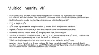
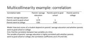
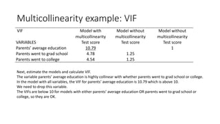
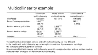
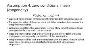
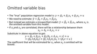
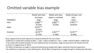
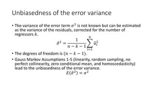
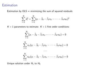
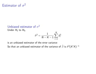
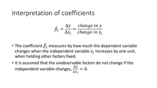
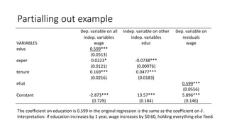
Econometrics Multiple Regression Model Slides

1. Multiple Linear Regression: Brief Overview

2. Multiple Linear Regression
Suppose we want to investigate the relation between:
I an outcome variable y
I a set of K explanatory variable x1, x2, . . . , xK
The Multiple Linear Regression model assumes that the following relation
is true in the population:
Population model
yi = β0 + β1x1i + β2x2i + · · · + βK xK + ui
I β0 is the value of y when all x’s and u equal zero
I βk is the effect of a unit-change in xk on y; it measures the marginal
effect of xk on y keeping u and the other x’s fixed

3. Multiple Linear Regression
I Adding other explanatory variables improves the goodness of fit
I Makes the Zero conditional mean assumption more credible:
wage = β0 + β1education + β2motivation + u
I Allows for other specifications:
wage = β0 + β1age + β2age2
+ u

4. Assumptions
H1 Linearity in parameters: y = β0 + β1x1 + β2x2 + · · · + βK xK + u
H2 Random sampling: (yi , xi1, . . . , xiK )i=1,...,N iid
H3 No perfect collinearity: xik 6= c and no linear relationship between
the x’s in the sample
H4 Zero conditional mean: E(u|x1, . . . , xK ) = E(u) = 0
H5 Homoscedasticity: Var(ui |x1, . . . , xK ) = σ2
, ∀i = 1, . . . , N

5. Estimation
Estimation by OLS = minimizing the sum of squared residuals:
N
X
i=1
û2
i =
N
X
i=1
(yi − β̂0 − β̂1x1i − · · · − β̂K xKi )2
K + 1 parameters to estimate: K + 1 first order conditions:
N
X
i=1
(yi − β̂0 − β̂1x1i − · · · − β̂K xKi ) = 0
N
X
i=1
x1i (yi − β̂0 − β̂1x1i − · · · − β̂K xKi ) = 0
. . .
N
X
i=1
xKi (yi − β̂0 − β̂1x1i − · · · − β̂K xKi ) = 0
Unique solution under H1 to H4

6. Interpretation of OLS estimates
I β̂0 ,β̂1, . . . , β̂K are partial effects
I β̂k is the effect of xk on y after the effect of other x’s on xk is
partialled out
I β̂k is the effect of xk on y, holding other x’s fixed
I Example:
wage = β0 + β1age + β2education + u
I β̂2 is the effect of schooling on wage that is not due to age, but only
to the level of schooling
I Ceteris paribus = everything else equal
I β̂2 is the effect of schooling when everything else (age here) is fixed,
and only the level of schooling varies

7. OLS in matrix form
I With multiple explanatory variables, it is easier to write the model in
matrix form:
y = Xβ + u
where
y =



y1
.
.
.
yN


 X =



1 x11 . . . xK1
.
.
.
.
.
.
...
.
.
.
1 x1N . . . xKN


 β =



β1
.
.
.
βK


 u =



u1
.
.
.
uN




8. OLS in matrix form
The K+1 first order conditions are simply:
X0
(y − Xβ̂) = 0
Which gives
β̂ = (X0
X)−1
X0
y

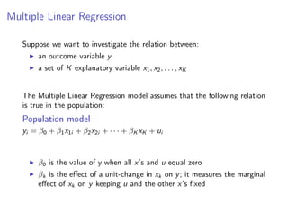
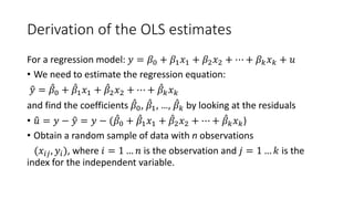
9. OLS in matrix form
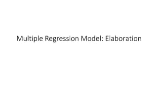
Unbiasedness follows from
E[β̂|X] = E[(X0
X)−1
X0
(Xβ + u)|X] = β + (X0
X)−1
X0
E[u|X] = β
under H1 to H4
From H5, the variance of the estimator is given by:
V [β̂|X] = E[(β̂ − β)(β̂ − β)0
]
= E[(X0
X)−1
X0
uu0
X(X0
X)−1
]
= (X0
X)−1
X0
E[uu0
|X]X(X0
X)−1
= (X0
X)−1
X0
σ2
IX(X0
X)−1
= σ2
(X0
X)−1

10. Estimator of σ2
Unbiased estimator of σ2
Under H1 to H5,
σ̂2
=
1
N − K − 1
N
X
i=1
û2
i
is an unbiased estimator of the error variance
So that an unbiased estimator of the variance of β̂ is σ̂2
(X0
X)−1

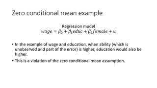
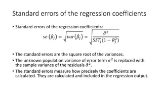
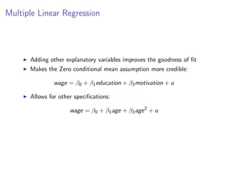
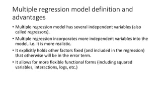
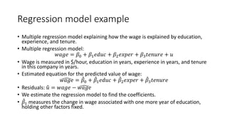
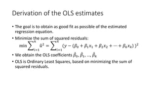
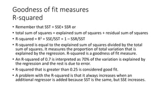
11. OLS is BLUE
Gauss-Markov Theorem
Under assumption H1 to H5, β̂ is the best linear unbiased estimator
(BLUE) of β
B Best = smallest variance
L Linear = β̂ is a linear combination of y
U Unbiased = E[β̂|X] = β
E Estimator

12. Multiple Regression Model: Elaboration

13. Multiple regression model definition and
advantages
• Multiple regression model has several independent variables (also
called regressors).
• Multiple regression incorporates more independent variables into the
model, i.e. it is more realistic.
• It explicitly holds other factors fixed (and included in the regression)
that otherwise will be in the error term.
• It allows for more flexible functional forms (including squared
variables, interactions, logs, etc.)

14. Terminology
Multiple regression model: 𝑦𝑦 = 𝛽𝛽0 + 𝛽𝛽1𝑥𝑥1 + 𝛽𝛽2𝑥𝑥2 + ⋯ + 𝛽𝛽𝑘𝑘𝑥𝑥𝑘𝑘 + 𝑢𝑢
𝑦𝑦 is dependent variable, 𝑥𝑥1, 𝑥𝑥2, … , 𝑥𝑥𝑘𝑘 are independent variables, 𝑢𝑢 is error, 𝛽𝛽0, 𝛽𝛽1, . . , 𝛽𝛽𝑘𝑘 are
parameters. There are 𝑘𝑘 independent variables.
𝑥𝑥𝑗𝑗 denotes any of the independent variables, and 𝛽𝛽𝑗𝑗 is its parameter, 𝑗𝑗 = 1 … 𝑘𝑘
Estimated equation: �
𝑦𝑦 = ̂
𝛽𝛽0 + ̂
𝛽𝛽1𝑥𝑥1 + ̂
𝛽𝛽2𝑥𝑥2 + ⋯ + ̂
𝛽𝛽𝑘𝑘𝑥𝑥𝑘𝑘
�
𝑦𝑦 is predicted value, ̂
𝛽𝛽0, ̂
𝛽𝛽1, …, ̂
𝛽𝛽𝑘𝑘 are coefficients,
𝑛𝑛 is the number of observations,
𝑖𝑖 is any of the observations, 𝑖𝑖 = 1 … 𝑛𝑛.
Residual: �
𝑢𝑢 = 𝑦𝑦 − �
𝑦𝑦
�
𝑢𝑢 = actual value minus predicted/fitted value for the dependent variable
Population Sample
Parameter 𝛽𝛽 Coefficient ̂
𝛽𝛽
Error 𝑢𝑢 Residual �
𝑢𝑢

15. Interpretation of coefficients
̂
𝛽𝛽𝑗𝑗 =
∆𝑦𝑦
∆𝑥𝑥𝑗𝑗
=
𝑐𝑐𝑐𝑐𝑐𝑐𝑐𝑐𝑐𝑐𝑐 𝑖𝑖𝑖𝑖 𝑦𝑦
𝑐𝑐𝑐𝑐𝑐𝑐𝑐𝑐𝑐𝑐𝑐 𝑖𝑖𝑖𝑖 𝑥𝑥𝑗𝑗
• The coefficient ̂
𝛽𝛽𝑗𝑗 measures by how much the dependent variable
changes when the independent variable 𝑥𝑥𝑗𝑗 increases by one unit,
when holding other factors fixed.
• It is assumed that the unobservable factors do not change if the
independent variable changes,
∆𝑢𝑢
∆𝑥𝑥𝑗𝑗
= 0.

16. Regression model example
• Multiple regression model explaining how the wage is explained by education,
experience, and tenure.
• Multiple regression model:
𝑤𝑤𝑤𝑤𝑤𝑤𝑤𝑤 = 𝛽𝛽0 + 𝛽𝛽1𝑒𝑒𝑒𝑒𝑒𝑒𝑒𝑒 + 𝛽𝛽2𝑒𝑒𝑒𝑒𝑒𝑒𝑒𝑒𝑒𝑒 + 𝛽𝛽3𝑡𝑡𝑡𝑡𝑡𝑡𝑡𝑡𝑡𝑡𝑡𝑡 + 𝑢𝑢
• Wage is measured in $/hour, education in years, experience in years, and tenure
in this company in years.
• Estimated equation for the predicted value of wage:
�
𝑤𝑤𝑤𝑤𝑤𝑤𝑤𝑤 = ̂
𝛽𝛽0 + ̂
𝛽𝛽1𝑒𝑒𝑒𝑒𝑒𝑒𝑒𝑒 + ̂
𝛽𝛽2𝑒𝑒𝑒𝑒𝑒𝑒𝑒𝑒𝑒𝑒 + ̂
𝛽𝛽3𝑡𝑡𝑡𝑡𝑡𝑡𝑡𝑡𝑡𝑡𝑡𝑡
• Residuals: �
𝑢𝑢 = 𝑤𝑤𝑤𝑤𝑤𝑤𝑤𝑤 − �
𝑤𝑤𝑤𝑤𝑤𝑤𝑤𝑤
• We estimate the regression model to find the coefficients.
• ̂
𝛽𝛽1 measures the change in wage associated with one more year of education,
holding other factors fixed.

17. Estimated equation and interpretation
• Estimated equation
�
𝑤𝑤𝑤𝑤𝑤𝑤𝑤𝑤 = ̂
𝛽𝛽0 + ̂
𝛽𝛽1𝑒𝑒𝑒𝑒𝑒𝑒𝑒𝑒 + ̂
𝛽𝛽2𝑒𝑒𝑒𝑒𝑒𝑒𝑒𝑒𝑒𝑒 + ̂
𝛽𝛽3𝑡𝑡𝑡𝑡𝑡𝑡𝑡𝑡𝑡𝑡𝑡𝑡
= −2.87 + 0.60 𝑒𝑒𝑒𝑒𝑒𝑒𝑒𝑒 + 0.02𝑒𝑒𝑒𝑒𝑒𝑒𝑒𝑒𝑒𝑒 + 0.17𝑡𝑡𝑡𝑡𝑡𝑡𝑡𝑡𝑡𝑡𝑡𝑡
• Wage is measured in $/hour, education in years, experience in years, and tenure in this
company in years.
• Interpretation of ̂
𝛽𝛽1: the hourly wage increases by $0.60 for each additional year of
education, holding other factors fixed.
• Interpretation of ̂
𝛽𝛽2: the hourly wage increases by $0.02 for each additional year of
experience, holding other factors fixed.
• Interpretation of ̂
𝛽𝛽3: the hourly wage increases by $0.17 for each additional year of
tenure in the company, holding other factors fixed.
• Interpretation of ̂
𝛽𝛽0: if all regressors are zero, a person’s wage is -$2.87 (but no one in
the sample has zero for all regressors).

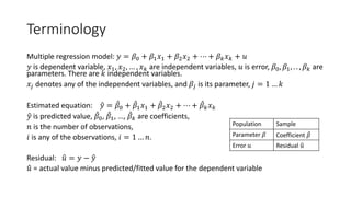
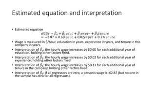
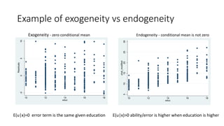
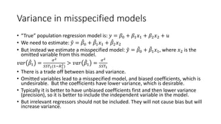
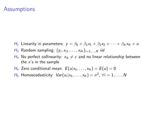
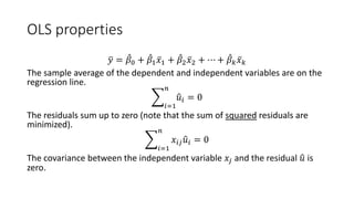
18. Stata output for multiple regression
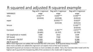
_cons -2.872735 .7289643 -3.94 0.000 -4.304799 -1.440671
tenure .1692687 .0216446 7.82 0.000 .1267474 .2117899
exper .0223395 .0120568 1.85 0.064 -.0013464 .0460254
educ .5989651 .0512835 11.68 0.000 .4982176 .6997126
wage Coef. Std. Err. t P>|t| [95% Conf. Interval]
Total 7160.41431 525 13.6388844 Root MSE = 3.0845
Adj R-squared = 0.3024
Residual 4966.30269 522 9.51398982 R-squared = 0.3064
Model 2194.11162 3 731.370541 Prob > F = 0.0000
F(3, 522) = 76.87
Source SS df MS Number of obs = 526
. regress wage educ exper tenure
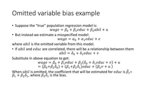
The coefficients are estimated with the Stata program.

19. Regression model example
Reg with 1 variable Reg with 2 variables Reg with 3 variables
VARIABLES wage wage wage
educ 0.541*** 0.644*** 0.599***
(0.0532) (0.0538) (0.0513)
exper 0.0701*** 0.0223*
(0.0110) (0.0121)
tenure 0.169***
(0.0216)
Constant -0.905 -3.391*** -2.873***
(0.685) (0.767) (0.729)
When education increases by 1 year, wage increases by $0.60, holding other factors fixed.
The coefficient on education changes slightly from one model to the next depending on
what other independent variables are included in the model.

20. Derivation of the OLS estimates
For a regression model: 𝑦𝑦 = 𝛽𝛽0 + 𝛽𝛽1𝑥𝑥1 + 𝛽𝛽2𝑥𝑥2 + ⋯ + 𝛽𝛽𝑘𝑘𝑥𝑥𝑘𝑘 + 𝑢𝑢
• We need to estimate the regression equation:
�
𝑦𝑦 = ̂
𝛽𝛽0 + ̂
𝛽𝛽1𝑥𝑥1 + ̂
𝛽𝛽2𝑥𝑥2 + ⋯ + ̂
𝛽𝛽𝑘𝑘𝑥𝑥𝑘𝑘
and find the coefficients ̂
𝛽𝛽0, ̂
𝛽𝛽1, …, ̂
𝛽𝛽𝑘𝑘 by looking at the residuals
• �
𝑢𝑢 = 𝑦𝑦 − �
𝑦𝑦 = 𝑦𝑦 − ( ̂
𝛽𝛽0 + ̂
𝛽𝛽1𝑥𝑥1 + ̂
𝛽𝛽2𝑥𝑥2 + ⋯ + ̂
𝛽𝛽𝑘𝑘𝑥𝑥𝑘𝑘)
• Obtain a random sample of data with n observations
(𝑥𝑥𝑖𝑖𝑖𝑖, 𝑦𝑦𝑖𝑖), where 𝑖𝑖 = 1 … 𝑛𝑛 is the observation and 𝑗𝑗 = 1 … 𝑘𝑘 is the
index for the independent variable.

21. Derivation of the OLS estimates
• The goal is to obtain as good fit as possible of the estimated
regression equation.
• Minimize the sum of squared residuals:
min �
𝑖𝑖=1
𝑛𝑛
�
𝑢𝑢2
= �
𝑖𝑖=1
𝑛𝑛
(𝑦𝑦 − (𝛽𝛽0 + 𝛽𝛽1𝑥𝑥1 + 𝛽𝛽2𝑥𝑥2 + ⋯ + 𝛽𝛽𝑘𝑘𝑥𝑥𝑘𝑘) )2
• We obtain the OLS coefficients ̂
𝛽𝛽0, ̂
𝛽𝛽1, …, ̂
𝛽𝛽𝑘𝑘
• OLS is Ordinary Least Squares, based on minimizing the sum of
squared residuals.

22. OLS properties
�
𝑦𝑦 = ̂
𝛽𝛽0 + ̂
𝛽𝛽1 ̅
𝑥𝑥1 + ̂
𝛽𝛽2 ̅
𝑥𝑥2 + ⋯ + ̂
𝛽𝛽𝑘𝑘 ̅
𝑥𝑥𝑘𝑘
The sample average of the dependent and independent variables are on the
regression line.
�
𝑖𝑖=1
𝑛𝑛
�
𝑢𝑢𝑖𝑖 = 0
The residuals sum up to zero (note that the sum of squared residuals are
minimized).
�
𝑖𝑖=1
𝑛𝑛
𝑥𝑥𝑖𝑖𝑖𝑖 �
𝑢𝑢𝑖𝑖 = 0
The covariance between the independent variable 𝑥𝑥𝑗𝑗 and the residual �
𝑢𝑢 is
zero.

23. Partialling out
• Partialling out shows an alternative way to obtain the regression
coefficient.
• Population regression model: 𝑦𝑦 = 𝛽𝛽0 + 𝛽𝛽1𝑥𝑥1 + 𝛽𝛽2𝑥𝑥2 + 𝛽𝛽3𝑥𝑥3 + 𝑢𝑢
• First regress the independent variable on all other independent variables:
𝑥𝑥1 = 𝛼𝛼0 + 𝛼𝛼2𝑥𝑥2 + 𝛼𝛼3𝑥𝑥3 + 𝑒𝑒
• Get the residuals from this regression: ̂
𝑒𝑒 = 𝑥𝑥1 − �
𝑥𝑥1 (showing the part of
the independent variable not explained by the other variables)
• Run the regression of the dependent variable on the residuals from this
regression to obtain the same coefficient: 𝑦𝑦 = 𝛾𝛾0 + 𝛽𝛽1 �
𝑒𝑒 + 𝑣𝑣
• The coefficient ̂
𝛽𝛽1 shows the relationship between 𝑦𝑦 and 𝑥𝑥1 that is not
explained by the other variables. This is why “holding everything else
fixed” is added when interpreting coefficients.

24. Partialling out example
Dep. variable on all
indep. variables
Indep. variable on other
indep. variables
Dep. variable on
residuals
VARIABLES wage educ wage
educ 0.599***
(0.0513)
exper 0.0223* -0.0738***
(0.0121) (0.00976)
tenure 0.169*** 0.0477***
(0.0216) (0.0183)
ehat 0.599***
(0.0556)
Constant -2.873*** 13.57*** 5.896***
(0.729) (0.184) (0.146)
The coefficient on education is 0.599 in the original regression is the same as the coefficient on ̂
𝑒𝑒.
Interpretation: if education increases by 1 year, wage increases by $0.60, holding everything else fixed.

25. Goodness of fit measures
R-squared
• Remember that SST = SSE+ SSR or
• total sum of squares = explained sum of squares + residual sum of squares
• R-squared = R2 = SSE/SST = 1 – SSR/SST
• R-squared is equal to the explained sum of squares divided by the total
sum of squares. It measures the proportion of total variation that is
explained by the regression. R-squared is a goodness of fit measure.
• An R-squared of 0.7 is interpreted as 70% of the variation is explained by
the regression and the rest is due to error.
• R-squared that is greater than 0.25 is considered good fit.
• A problem with the R-squared is that it always increases when an
additional regressor is added because SST is the same, but SSE increases.

26. Adjusted R-squared
• The adjusted R-squared is an R-squared that has been adjusted for the number of
regressors in the model. The adjusted R-squared increases only if the new regressor
improves the model.
• Recall that R-squared = 𝑅𝑅2= 1 −
𝑆𝑆𝑆𝑆𝑆𝑆
𝑆𝑆𝑆𝑆𝑆𝑆
• Adjusted R-squared = Adj 𝑅𝑅2
= 1 −
𝑆𝑆𝑆𝑆𝑆𝑆/(𝑛𝑛−𝑘𝑘−1)
𝑆𝑆𝑆𝑆𝑆𝑆/(𝑛𝑛−1)
• where n is the number of observations and k is the number of independent variables.
• Adjusted R-squared = 1 − (1 − 𝑅𝑅2
)(𝑛𝑛 − 1)/(𝑛𝑛 − 𝑘𝑘 − 1)
• As the number of regressors k increases, the adjusted R-squared would be penalized.
• When adding more regressors, the adjusted R2 may increase but it also may decrease or
even get negative.
• Rule: choose a model with higher adjusted R-squared when deciding whether to keep a
variable or not in the model.

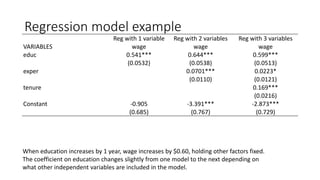
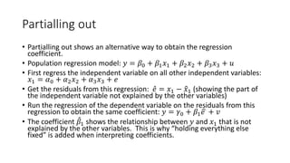
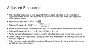
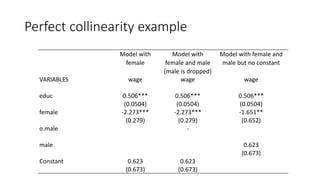
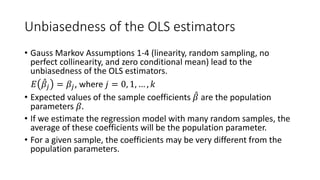
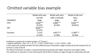
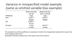
27. Adjusted R-squared calculation
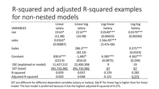
R-squared = SS Model /SS Total = 2194 / 7160 = 1 – SSR/SST = 1 – 4966/7160 = 0.306
Adj R-squared = 1 – [SSR/(n-k-1)] / [SST/(n-1)] = 1 – (4966/522)/ (7160/525) = 0.302
30% of the variation in wage is explained by the regression and the rest is due to error.
_cons -2.872735 .7289643 -3.94 0.000 -4.304799 -1.440671
tenure .1692687 .0216446 7.82 0.000 .1267474 .2117899
exper .0223395 .0120568 1.85 0.064 -.0013464 .0460254
educ .5989651 .0512835 11.68 0.000 .4982176 .6997126
wage Coef. Std. Err. t P>|t| [95% Conf. Interval]
Total 7160.41431 525 13.6388844 Root MSE = 3.0845
Adj R-squared = 0.3024
Residual 4966.30269 522 9.51398982 R-squared = 0.3064
Model 2194.11162 3 731.370541 Prob > F = 0.0000
F(3, 522) = 76.87
Source SS df MS Number of obs = 526

28. R-squared and adjusted R-squared example
Reg with 1 regressor Reg with 2 regressor Reg with 3 regressor
VARIABLES wage wage wage
educ 0.541*** 0.644*** 0.599***
(0.0532) (0.0538) (0.0513)
exper 0.0701*** 0.0223*
(0.0110) (0.0121)
tenure 0.169***
(0.0216)
Constant -0.905 -3.391*** -2.873***
(0.685) (0.767) (0.729)
SSE (explained or model) 1180 1612 2194
SST (total) 7160 7160 7160
R-squared = SSE/SST 0.165 0.225 0.306
Adj R-squared 0.163 0.222 0.302
When more regressors are added, SSE increases but SST is the same. So R-squared always increases
when more variables are added (the regression can explain more of the total variation).
Adjusted R-squared can increase or decrease as more variables are added. Here, the most desirable model with the
highest adj R-squared of 0.3 (explaining 30% of the variation) is the model with 3 regressors.

29. R-squared and adjusted R-squared examples
for non-nested models
Linear Linear-log Log-linear Log-log
VARIABLES salary salary lsalary lsalary
roe 19.63* 22.67** 0.0149*** 0.0179***
(11.08) (10.98) (0.00433) (0.00396)
sales 0.0163* 1.56e-05***
(0.00887) (3.47e-06)
lsales 286.3*** 0.275***
(92.33) (0.0333)
Constant 830.6*** -1,482* 6.585*** 4.362***
(223.9) (816.0) (0.0875) (0.294)
SSE (explained or model) 11,427,512 22,400,308 9 19
SST (total) 391,732,982 391,732,982 67 67
R-squared 0.029 0.057 0.129 0.282
Adjusted R-squared 0.020 0.048 0.121 0.275
SST are different for different dependent variables (salary vs lsalary). Adj R2 for linear-log is higher than for linear
model. The last model is preferred because it has the highest adjusted R-squared of 0.275.

30. Gauss Markov assumptions
• Gauss Markov assumptions are standard assumptions for the linear
regression model
1. Linearity in parameters
2. Random sampling
3. No perfect collinearity
4. Zero conditional mean (exogeneity) – regressors are not correlated
with the error term
5. Homoscedasticity – variance of error term is constant

31. Assumption 1: linearity in parameters
𝑦𝑦 = 𝛽𝛽0 + 𝛽𝛽1𝑥𝑥1 + 𝛽𝛽2𝑥𝑥2 + ⋯ + 𝛽𝛽𝑘𝑘𝑥𝑥𝑘𝑘 + 𝑢𝑢
• The relationship between the dependent and independent variables
is linear in the population.
• Note that the regression model can have logged variables (e.g. log
sales), squared variables (e.g. education2) or interactions of variables
(e.g. education*experience) but the 𝛽𝛽 parameters are linear.

32. Assumption 2: random sampling
𝑦𝑦𝑖𝑖 = 𝛽𝛽0 + 𝛽𝛽1𝑥𝑥𝑖𝑖1 + 𝛽𝛽2𝑥𝑥𝑖𝑖2 + ⋯ + 𝛽𝛽𝑘𝑘𝑥𝑥𝑖𝑖𝑘𝑘 + 𝑢𝑢𝑖𝑖
𝑥𝑥𝑖𝑖𝑖, 𝑥𝑥𝑖𝑖𝑖, … , 𝑥𝑥𝑖𝑖𝑖𝑖, 𝑦𝑦𝑖𝑖 , where 𝑖𝑖= 1….n
• The data are a random sample drawn from the population. Each
observation has an equal probability of being selected.
• Each observation follows the population equation.

33. Assumption 3: no perfect collinearity
• No perfect collinearity - none of the independent variables are constant and
there are no exact relationships among them.
• An independent variable cannot be a constant because it will be collinear with
the constant/intercept in the model.
• An independent variable cannot be a perfect linear combination of other
independent variables (perfect collinearity). It must be dropped from the model.
• Independent variables can still be highly correlated with each other
(multicollinearity), which is not a violation of this assumption though
multicollinearity is also problematic.
• If independent variables are in shares that sum up to 100% (e.g. proportion of
income spent on food and proportion of income not spent on food), one of the
variables must be dropped. But income spent on food and income not spent on
food do not sum up to 100% so both variables can be used in the model.

34. Perfect collinearity example
• Model with female
𝑤𝑤𝑤𝑤𝑤𝑤𝑤𝑤 = 𝛽𝛽0 + 𝛽𝛽1𝑒𝑒𝑒𝑒𝑒𝑒𝑒𝑒 + 𝛽𝛽2𝑓𝑓𝑓𝑓𝑓𝑓𝑓𝑓𝑓𝑓𝑓𝑓 + 𝑢𝑢
• Model with female and male
𝑤𝑤𝑤𝑤𝑤𝑤𝑤𝑤 = 𝛽𝛽0 + 𝛽𝛽1𝑒𝑒𝑒𝑒𝑒𝑒𝑒𝑒 + 𝛽𝛽2𝑓𝑓𝑓𝑓𝑓𝑓𝑓𝑓𝑓𝑓𝑓𝑓 + 𝛽𝛽3𝑚𝑚𝑚𝑚𝑚𝑚𝑚𝑚 + 𝑢𝑢
where 𝑚𝑚𝑚𝑚𝑚𝑚𝑚𝑚 = 1 − 𝑓𝑓𝑓𝑓𝑓𝑓𝑓𝑓𝑓𝑓𝑓𝑓
This model cannot be estimated because female and male are perfectly
collinear. Solution:
- Drop the collinear variable 𝑚𝑚𝑚𝑚𝑚𝑚𝑚𝑚
- Drop the constant (not commonly used)

35. Perfect collinearity example
Model with
female
Model with
female and male
(male is dropped)
Model with female and
male but no constant
VARIABLES wage wage wage
educ 0.506*** 0.506*** 0.506***
(0.0504) (0.0504) (0.0504)
female -2.273*** -2.273*** -1.651**
(0.279) (0.279) (0.652)
o.male -
male 0.623
(0.673)
Constant 0.623 0.623
(0.673) (0.673)

36. Multicollinearity: VIF
• Multicollinearity is when two or more independent variables are highly linearly related
(correlated) with each other. The solution is to remove some of the variables or combine them.
• Multicollinearity can be checked by using variance inflation factors (VIF)
• 𝑉𝑉𝑉𝑉𝑉𝑉𝑗𝑗 = 1/(1 − 𝑅𝑅𝑗𝑗
2
)
• 𝑅𝑅𝑗𝑗
2
is the R-squared from a regression of 𝑥𝑥𝑗𝑗 on the other independent variables.
• Higher 𝑅𝑅𝑗𝑗
2
would mean that 𝑥𝑥𝑗𝑗 is well explained by other independent variables.
• From the formula above, when 𝑅𝑅𝑗𝑗
2
is higher, then 𝑉𝑉𝑉𝑉𝑉𝑉𝑗𝑗 will be higher.
• The rule of thumb is to drop variable 𝑥𝑥𝑗𝑗 if 𝑉𝑉𝑉𝑉𝑉𝑉𝑗𝑗 > 10, which means that 𝑅𝑅𝑗𝑗
2
> 0.9. This variable
would be well explained by the other variables in the model.
• VIF=1 for simple regression because there are no other variables and 𝑅𝑅𝑗𝑗
2
= 0
• Another rule of thumb is to drop a variable if it has a correlation coefficient above 0.9 with
another variable. But it is better to use VIF for multicollinearity among all independent variables
instead of correlation coefficient between two variables.

37. Multicollinearity example: correlation
Correlation table Parents’ average
education
Parents went to grad
school
Parents went to
college
Parents’ average education 1
Parents went to grad school 0.79 1
Parents went to college 0.81 0.42 1
Model: how test scores of a student depend on parents’ average education and whether parents
went to grad school or college.
First, find the correlation between two variables at a time.
The variable of parents’ average education is highly correlated with whether parents
went to grad school or college; the correlation coefficients are 0.79 and 0.81.

38. Multicollinearity example: VIF
VIF Model with
multicollinearity
Model without
multicollinearity
Model without
multicollinearity
VARIABLES Test score Test score Test score
Parents’ average education 10.79 1
Parents went to grad school 4.78 1.25
Parents went to college 4.54 1.25
Next, estimate the models and calculate VIF.
The variable parents’ average education is highly collinear with whether parents went to grad school or college.
In the model with all variables, the VIF for parents’ average education is 10.79 which is above 10.
We need to drop this variable.
The VIFs are below 10 for models with either parents’ average education OR parents went to grad school or
college, so they are OK.

39. Multicollinearity example
Model with
multicollinearity
Model without
multicollinearity
Model without
multicollinearity
VARIABLES Test score Test score Test score
Parents’ average education 203.9*** 148.2***
(18.78) (5.847)
Parents went to grad school -1.091 5.829***
(0.758) (0.475)
Parents went to college -2.426*** 2.648***
(0.587) (0.350)
Constant 162.7*** 545.1*** 251.4***
The coefficients in the models without and with multicollinearity are very different.
In the model with multicollinearity we can wrongly conclude that if parents went to college,
the test scores of the student will be lower.
Drop the variable that is causing multicollinearity (parents’ average education) and use last two models.
Standard errors are higher for model with multicollinearity.

40. Assumption 4: zero conditional mean
(exogeneity)
𝐸𝐸 𝑢𝑢𝑖𝑖 𝑥𝑥𝑖𝑖𝑖, 𝑥𝑥𝑖𝑖𝑖, … , 𝑥𝑥𝑖𝑖𝑖𝑖) = 0
• Expected value of error term 𝑢𝑢 given the independent variables 𝑥𝑥 is zero.
• The expected value of the error must not differ based on the values of the
independent variables.
• With more variables, this assumption is more likely to hold because fewer
unobservable factors are in the error term.
• Independent variables that are correlated with the error term are called
endogenous; endogeneity is a violation of this assumption.
• Independent variables that are uncorrelated with the error term are called
exogenous; this assumption holds if all independent variables are
exogenous.

41. Zero conditional mean example
Regression model
𝑤𝑤𝑤𝑤𝑤𝑤𝑤𝑤 = 𝛽𝛽0 + 𝛽𝛽1𝑒𝑒𝑒𝑒𝑒𝑒𝑒𝑒 + 𝛽𝛽2𝑓𝑓𝑓𝑓𝑓𝑓𝑓𝑓𝑓𝑓𝑓𝑓 + 𝑢𝑢
• In the example of wage and education, when ability (which is
unobserved and part of the error) is higher, education would also be
higher.
• This is a violation of the zero conditional mean assumption.

42. Example of exogeneity vs endogeneity
-5
0
5
10
Residuals
10 12 14 16 18
educ
5
10
15
20
25
30
uhat_modified
10 12 14 16 18
educ
E(u|x)=0 error term is the same given education E(u|x)>0 ability/error is higher when education is higher
Exogeneity - zero conditional mean Endogeneity - conditional mean is not zero

43. Unbiasedness of the OLS estimators
• Gauss Markov Assumptions 1-4 (linearity, random sampling, no
perfect collinearity, and zero conditional mean) lead to the
unbiasedness of the OLS estimators.
𝐸𝐸 ̂
𝛽𝛽𝑗𝑗 = 𝛽𝛽𝑗𝑗, where 𝑗𝑗 = 0, 1, … , 𝑘𝑘
• Expected values of the sample coefficients ̂
𝛽𝛽 are the population
parameters 𝛽𝛽.
• If we estimate the regression model with many random samples, the
average of these coefficients will be the population parameter.
• For a given sample, the coefficients may be very different from the
population parameters.

44. Omitted variable bias
• The “true” population regression model is: 𝑦𝑦 = 𝛽𝛽0 + 𝛽𝛽1𝑥𝑥1 + 𝛽𝛽2𝑥𝑥2 + 𝑢𝑢
• We need to estimate: �
𝑦𝑦 = ̂
𝛽𝛽0 + ̂
𝛽𝛽1𝑥𝑥1 + ̂
𝛽𝛽2𝑥𝑥2
• But instead we estimate a misspecified model: �
𝑦𝑦 = �
𝛽𝛽0 + �
𝛽𝛽1𝑥𝑥1, where 𝑥𝑥2 is
the omitted variable from this model.
• If 𝑥𝑥1and 𝑥𝑥2 are correlated, there will be a relationship between them
𝑥𝑥2 = 𝛿𝛿0 + 𝛿𝛿1𝑥𝑥1 + 𝑣𝑣
Substitute in above equation to get:
𝑦𝑦 = 𝛽𝛽0 + 𝛽𝛽1𝑥𝑥1 + 𝛽𝛽2 𝛿𝛿0 + 𝛿𝛿1𝑥𝑥1 + 𝑣𝑣 + 𝑢𝑢
= (𝛽𝛽0+𝛽𝛽2𝛿𝛿0) + (𝛽𝛽1+𝛽𝛽2𝛿𝛿1)𝑥𝑥1 + 𝛽𝛽2𝑣𝑣 + 𝑢𝑢
The coefficient that will be estimated for 𝑥𝑥1 when 𝑥𝑥2 is omitted will be
biased.

45. Omitted variable bias
• An unbiased coefficient is when 𝐸𝐸 ̂
𝛽𝛽1 = 𝛽𝛽1, but this coefficient is
biased because 𝐸𝐸 �
𝛽𝛽1 = 𝛽𝛽1 +𝛽𝛽2 𝛿𝛿1, where 𝛽𝛽2𝛿𝛿1 is the bias.
• With an omitted variable, the coefficient will not be biased if
• 𝛽𝛽2 = 0. Looking at 𝑦𝑦 = 𝛽𝛽0 + 𝛽𝛽1𝑥𝑥1 + 𝛽𝛽2𝑥𝑥2 + 𝑢𝑢, this means that 𝑥𝑥2 does not
belong in the model (𝑥𝑥2 is irrelevant).
• 𝛿𝛿1 = 0. Looking at 𝑥𝑥2 = 𝛿𝛿0 + 𝛿𝛿1𝑥𝑥1 + 𝑣𝑣, this means that 𝑥𝑥2 and 𝑥𝑥1are not
correlated.
• In other words, if the omitted variable is irrelevant 𝛽𝛽2 = 0 or uncorrelated
𝛿𝛿1 = 0, there will be no omitted variable bias.

46. Omitted variable bias example
• Suppose the “true” population regression model is:
𝑤𝑤𝑤𝑤𝑤𝑤𝑤𝑤 = 𝛽𝛽0 + 𝛽𝛽1𝑒𝑒𝑒𝑒𝑒𝑒𝑒𝑒 + 𝛽𝛽2𝑎𝑎𝑎𝑎𝑎𝑎𝑎𝑎 + 𝑢𝑢
• But instead we estimate a misspecified model:
𝑤𝑤𝑤𝑤𝑤𝑤𝑤𝑤 = 𝛼𝛼0 + 𝛼𝛼1𝑒𝑒𝑒𝑒𝑒𝑒𝑒𝑒 + 𝑒𝑒
where 𝑎𝑎𝑏𝑏𝑏𝑏𝑏𝑏 is the omitted variable from this model.
• If 𝑎𝑎𝑎𝑎𝑎𝑎𝑎𝑎 and 𝑒𝑒𝑒𝑒𝑒𝑒𝑒𝑒 are correlated, there will be a relationship between them
𝑎𝑎𝑎𝑎𝑎𝑎𝑎𝑎 = 𝛿𝛿0 + 𝛿𝛿1𝑒𝑒𝑒𝑒𝑒𝑒𝑒𝑒 + 𝑣𝑣
Substitute in above equation to get:
𝑤𝑤𝑤𝑤𝑤𝑤𝑤𝑤 = 𝛽𝛽0 + 𝛽𝛽1𝑒𝑒𝑒𝑒𝑒𝑒𝑒𝑒 + 𝛽𝛽2 𝛿𝛿0 + 𝛿𝛿1𝑒𝑒𝑒𝑒𝑒𝑒𝑒𝑒 + 𝑣𝑣 + 𝑢𝑢
= (𝛽𝛽0+𝛽𝛽2𝛿𝛿0) + (𝛽𝛽1+𝛽𝛽2𝛿𝛿1)𝑒𝑒𝑒𝑒𝑒𝑒𝑒𝑒 + 𝛽𝛽2𝑣𝑣 + 𝑢𝑢
When 𝑎𝑎𝑎𝑎𝑎𝑎𝑎𝑎 is omitted, the coefficient that will be estimated for 𝑒𝑒𝑒𝑒𝑒𝑒𝑒𝑒 is �
𝛽𝛽1=
𝛽𝛽1 + 𝛽𝛽2𝛿𝛿1, where 𝛽𝛽2𝛿𝛿1 is the bias.

47. Omitted variable bias example
Model with educ
and abil
Model with educ
(abil is omitted)
Model of abil and
educ
VARIABLES wage wage abil
educ 1.153*** 1.392*** 0.551***
(0.127) (0.103) (0.0213)
abil 0.433***
(0.137)
Constant -2.523 -4.857*** -5.389***
(1.543) (1.360) (0.282)
Coefficient in model with omitted variable = 𝛽𝛽�1biased =
= original coefficient + bias = 𝛽𝛽̂1 + 𝛽𝛽̂2𝛿𝛿̂1 = 1.153 + 0.433*0.551 = 1.153 + 0.238 = 1.392
In the model with omitted variable, for each additional year of education, wage increases by $1.39 instead of $1.15,
so there is a bias of $0.24.
The effect of education on wage is overestimated because people with higher education have higher ability.
The coefficient on education is also reflecting the $0.24 effect of ability on wage through its relationship with ed
. u

48. Omitted variable bias example
Model with educ
and exper
Model with educ
(exper is omitted)
Model of exper and
educ
VARIABLES wage wage exper
educ 1.948*** 1.392*** -0.905***
(0.139) (0.103) (0.0275)
exper 0.614***
(0.105)
Constant -18.70*** -4.857*** 22.54***
(2.724) (1.360) (0.364)
Now, suppose that we have experience instead of ability for the true model.
Coefficient in model with omitted variable = 1.392 = original coefficient + bias = 1.948 + 0.614*(-0.905)= 1.948-0.556
In the model with omitted variable, for each additional year of education, wage increases by $1.39 instead of $1.95,
so there is a negative bias of -$0.56.
The effect of education on wage is underestimated because people with higher education have less experience.
The coefficient on education is also reflecting the -$0.56 effect of experience on wage through its relationship with educ.

49. Including irrelevant variables
• Suppose the “true” population regression model is:
𝑦𝑦 = 𝛽𝛽0 + 𝛽𝛽1𝑥𝑥1 + 𝛽𝛽2𝑥𝑥2 + 𝑢𝑢
• But instead we estimate a misspecified model:
𝑦𝑦 = 𝛽𝛽0 + 𝛽𝛽1𝑥𝑥1 + 𝛽𝛽2𝑥𝑥2 + 𝛽𝛽3𝑥𝑥3 + 𝑒𝑒
where 𝑥𝑥3 is an irrelevant variable that is included.
• In the population regression model, 𝐸𝐸 ̂
𝛽𝛽3 = 𝛽𝛽3 = 0 because the
variable is not included.
• Adding an irrelevant variable does not cause bias but it increases the
sampling variance.

50. Assumption 5: homoscedasticity
• Homoscedasticity 𝑣𝑣𝑣𝑣𝑣𝑣 𝑢𝑢𝑖𝑖 𝑥𝑥𝑖𝑖𝑖, 𝑥𝑥𝑖𝑖2, … , 𝑥𝑥𝑖𝑖𝑘𝑘 = 𝜎𝜎2
• Variance of the error term 𝑢𝑢 must not differ with the independent
variables.
• Heteroscedasticity 𝑣𝑣𝑣𝑣𝑣𝑣 𝑢𝑢𝑖𝑖 𝑥𝑥𝑖𝑖𝑖, 𝑥𝑥𝑖𝑖𝑖, … , 𝑥𝑥𝑖𝑖𝑖𝑖 ≠ 𝜎𝜎2
is when the variance
of the error term 𝑢𝑢 is not constant for each 𝑥𝑥.

51. Homoscedasticity vs heteroscedasticity
example
-10
-5
0
5
10
15
Residuals
0 5 10 15 20
educ
-10
-5
0
5
10
15
Residuals,
uhat
0 10 20 30 40 50
exper
Homoscedasticity for experience
𝑣𝑣𝑣𝑣𝑣𝑣 𝑢𝑢 𝑒𝑒𝑒𝑒𝑒𝑒𝑒𝑒𝑒𝑒 = 𝜎𝜎2
Heteroscedasticity for education
𝑣𝑣𝑣𝑣𝑣𝑣 𝑢𝑢 𝑒𝑒𝑒𝑒𝑒𝑒𝑒𝑒 ≠ 𝜎𝜎2

52. Variances of the OLS estimators
Recall with simple regression: 𝑣𝑣𝑣𝑣𝑣𝑣 ̂
𝛽𝛽1 =
𝜎𝜎2
𝑆𝑆𝑆𝑆𝑇𝑇𝑥𝑥
With multiple regression: 𝑣𝑣𝑣𝑣𝑣𝑣 ̂
𝛽𝛽𝑗𝑗 =
𝜎𝜎2
𝑆𝑆𝑆𝑆𝑇𝑇𝑗𝑗(1−𝑅𝑅𝑗𝑗
2)
• 𝑆𝑆𝑆𝑆𝑇𝑇𝑗𝑗 = ∑𝑖𝑖=1
𝑛𝑛
(𝑥𝑥𝑖𝑖𝑗𝑗 − ̅
𝑥𝑥𝑗𝑗)2
is the total sampling variance of variable 𝑥𝑥𝑗𝑗. High variance of the
regressor will lead to lower variance of the coefficient.
• 𝑅𝑅𝑗𝑗
2
is the R-squared from a regression of 𝑥𝑥𝑗𝑗 on all other independent variables. High R-
squared means that the regressor is very well explained by other regressors
(multicollinearity) and it will have higher variance of its coefficient.
• 𝜎𝜎2
is the variance of the error term. High variance in the error term will lead to high
variance of the coefficients.
• Estimators with lower variance are also called more precise and are desirable. This
means that high variance in the independent variable, low R-squared for 𝑥𝑥𝑗𝑗 (less
multicollinearity), and low variance in the error term are desirable.

53. Unbiasedness of the error variance
• The variance of the error term 𝜎𝜎2
is not known but can be estimated
as the variance of the residuals, corrected for the number of
regressors 𝑘𝑘.
�
𝜎𝜎2
=
1
𝑛𝑛 − 𝑘𝑘 − 1
�
𝑖𝑖=1
𝑛𝑛
�
𝑢𝑢𝑖𝑖
2
• The degrees of freedom is (𝑛𝑛 − 𝑘𝑘 − 1).
• Gauss Markov Assumptions 1-5 (linearity, random sampling, no
perfect collinearity, zero conditional mean, and homoscedasticity)
lead to the unbiasedness of the error variance.
𝐸𝐸 �
𝜎𝜎2
= 𝜎𝜎2

54. Standard errors of the regression coefficients
• Standard errors of the regression coefficients:
𝑠𝑠𝑠𝑠 ̂
𝛽𝛽𝑗𝑗 = 𝑣𝑣𝑣𝑣𝑣𝑣 ̂
𝛽𝛽𝑗𝑗 =
�
𝜎𝜎2
𝑆𝑆𝑆𝑆𝑇𝑇𝑗𝑗(1 − 𝑅𝑅𝑗𝑗
2
)
• The standard errors are the square root of the variances.
• The unknown population variance of error term 𝜎𝜎2
is replaced with
the sample variance of the residuals �
𝜎𝜎2
.
• The standard errors measure how precisely the coefficients are
calculated. They are calculated and included in the regression output.

55. Variance in misspecified models
• “True” population regression model is: 𝑦𝑦 = 𝛽𝛽0 + 𝛽𝛽1𝑥𝑥1 + 𝛽𝛽2𝑥𝑥2 + 𝑢𝑢
• We need to estimate: �
𝑦𝑦 = ̂
𝛽𝛽0 + ̂
𝛽𝛽1𝑥𝑥1 + ̂
𝛽𝛽2𝑥𝑥2
• But instead we estimate a misspecified model: �
𝑦𝑦 = �
𝛽𝛽0 + �
𝛽𝛽1𝑥𝑥1, where 𝑥𝑥2 is the
omitted variable from this model.
𝑣𝑣𝑣𝑣𝑣𝑣 ̂
𝛽𝛽1 =
𝜎𝜎2
𝑆𝑆𝑆𝑆𝑇𝑇1(1−𝑅𝑅1
2)
> 𝑣𝑣𝑣𝑣𝑣𝑣 �
𝛽𝛽1 =
𝜎𝜎2
𝑆𝑆𝑆𝑆𝑇𝑇1
• There is a trade off between bias and variance.
• Omitted variables lead to a misspecified model, and biased coefficients, which is
undesirable. But the coefficients have lower variance, which is desirable.
• Typically it is better to have unbiased coefficients first and then lower variance
(precision), so it is better to include the independent variable in the model.
• But irrelevant regressors should not be included. They will not cause bias but will
increase variance.

56. Variance in misspecified model example
(same as omitted variable bias example)
Model with educ
and abil
Model with educ
(abil is omitted)
VARIABLES wage wage
educ 1.153*** 1.392***
(0.127) (0.103)
abil 0.433***
(0.137)
Constant -2.523 -4.857***
(1.543) (1.360)
The standard error of the coefficient on education is 0.103 in the misspecified model which is lower than
in the original model 0.127.
Remember that the standard error is the square root of the variance.

57. Gauss-Markov theorem
• Gauss Markov theorem says that under assumptions 1-5 (linearity in
parameters, random sampling, no perfect collinearity, zero
conditional mean, homoscedasticity), the OLS estimators are best
linear unbiased estimators (BLUE) of the coefficients.
• Estimators are linear in the dependent variable.
̂
𝛽𝛽𝑗𝑗 = ∑𝑖𝑖=1
𝑛𝑛
𝑤𝑤𝑖𝑖𝑖𝑖𝑦𝑦𝑖𝑖, for example in simple regression ̂
𝛽𝛽1 =
∑(𝑥𝑥𝑖𝑖− ̅
𝑥𝑥)(𝑦𝑦𝑖𝑖− �
𝑦𝑦)
∑(𝑥𝑥𝑖𝑖− ̅
𝑥𝑥)2
• From all linear estimators, OLS estimators have the lowest variance
(best means lowest variance).