1. The optimal input blend is where the marginal productivity per dollar spent is equal for all inputs. 2. A production function specifies the maximum output possible from different combinations of inputs. 3. A cost minimizing firm will produce at the input levels where the marginal costs of each input are equal to its price.

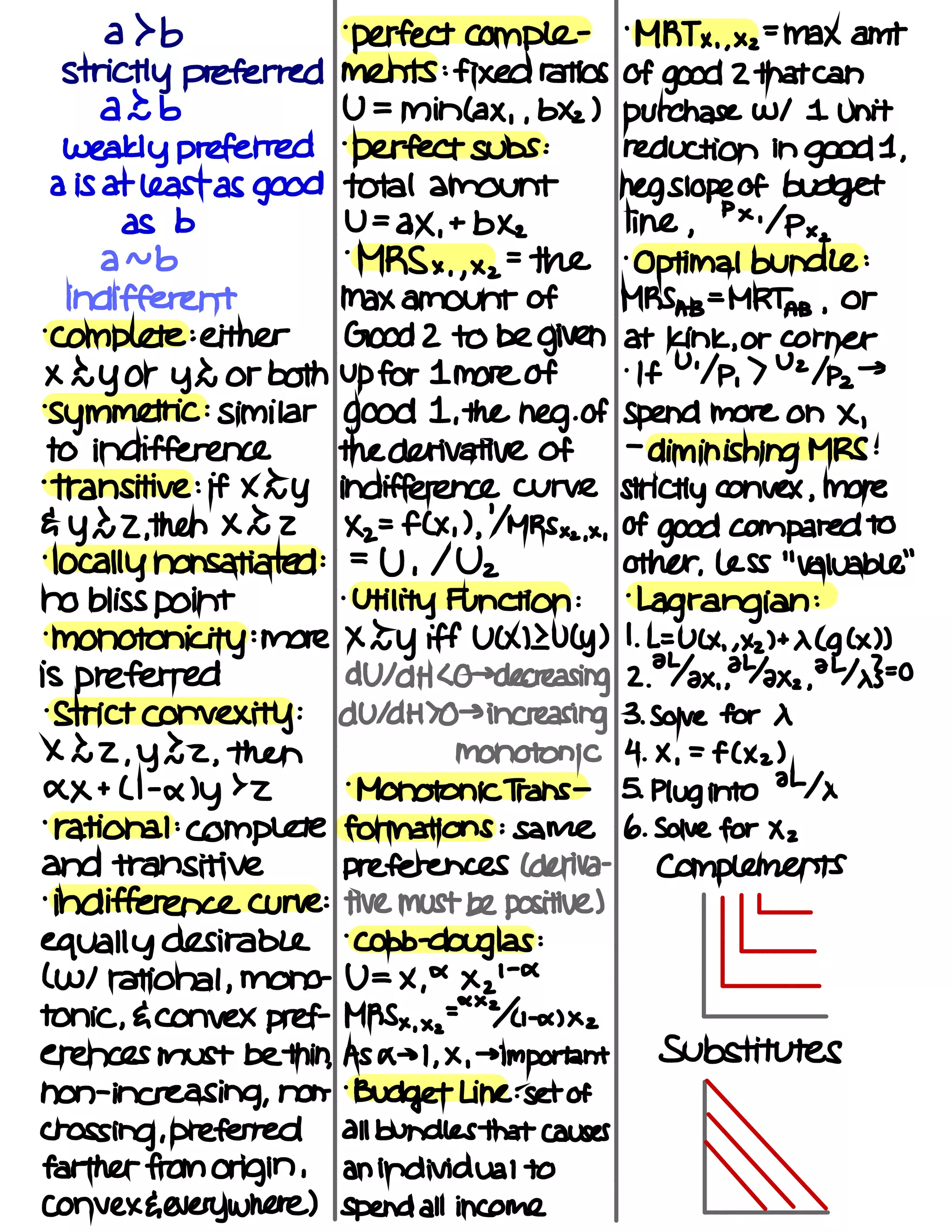
1. a > b
.
perfect Compte -
.
MRTX . ,×z=maxamt
Strictly preferred merits :
fixed ratios of good Zthatcan
a Ib
U=mih(
ax , ,bXz ) purchase WII unit
weakly preferred
.
perfect subs :
reduction in
good 't ,
a is atleast as good total amount negslopeof budget
as b
U=aX
,
tbxz line ,
Px .
/p× a
a~b
.
MRS , , ,×z= the .
Optimal bundle :
indifferent Max amount of MRSAPEMRTAB .
Or
.
Complete : either Good 2 to be given at kink ,
or corner
xdyoryhorbothupfor1moreof.HU/p,7V2/pz-s
.
Symmetric :
similar good 1. the
neg . of Spend more on X ,
to indifference the derivative of -
diminishing MRS :
-
transitive :ifXdy indifference curve
strictly convex ,
more
E.
yd 2. then Xd 2 Xz=fCX ,
) ,
'/MRS×a,×,
Of
good compared to
.
locally nonsatiated : =
U , 102 other ,
less
"
Valuable
"
no bliss point
.
Utility Function :
.
Lagrangian :
.
Monotonicity :
more X1yiff UNRULY ) 1. L= UH . ,xzHXLgCx ) )
is preferred DUIDHLO →
decreasing
2942×942×2,24×3=0
.
Strict convexity : dUldH70→ increasing 3. Solve for X
X 12,412 ,
then monotonic 4. X. =
f C Xz )
XX t LI -
a) y
> 2
.
Monotonic Trans -
5.
Plug into Mx
.
rational :
complete formations : same 6. Solve for Xz
and transitive preferences L derma -
Complements
.
indifference curve :
five must be positive )
equally desirable
.
Cobb -
douglas :
( w/ rational ,
mono -
U= X.
a
Xz
' -
a
tonic ,
E convex pref -
MRSx.x.FM/u.asxzerencesmustbethin.Asa-
1. x. →
important Substitutes
non -
increasing ,
non -
.
Budget Line :
set of
crossing , preferred all bundles that causes
farther from origin , an individual to
convex E. everywhere ) spend all income

2. -
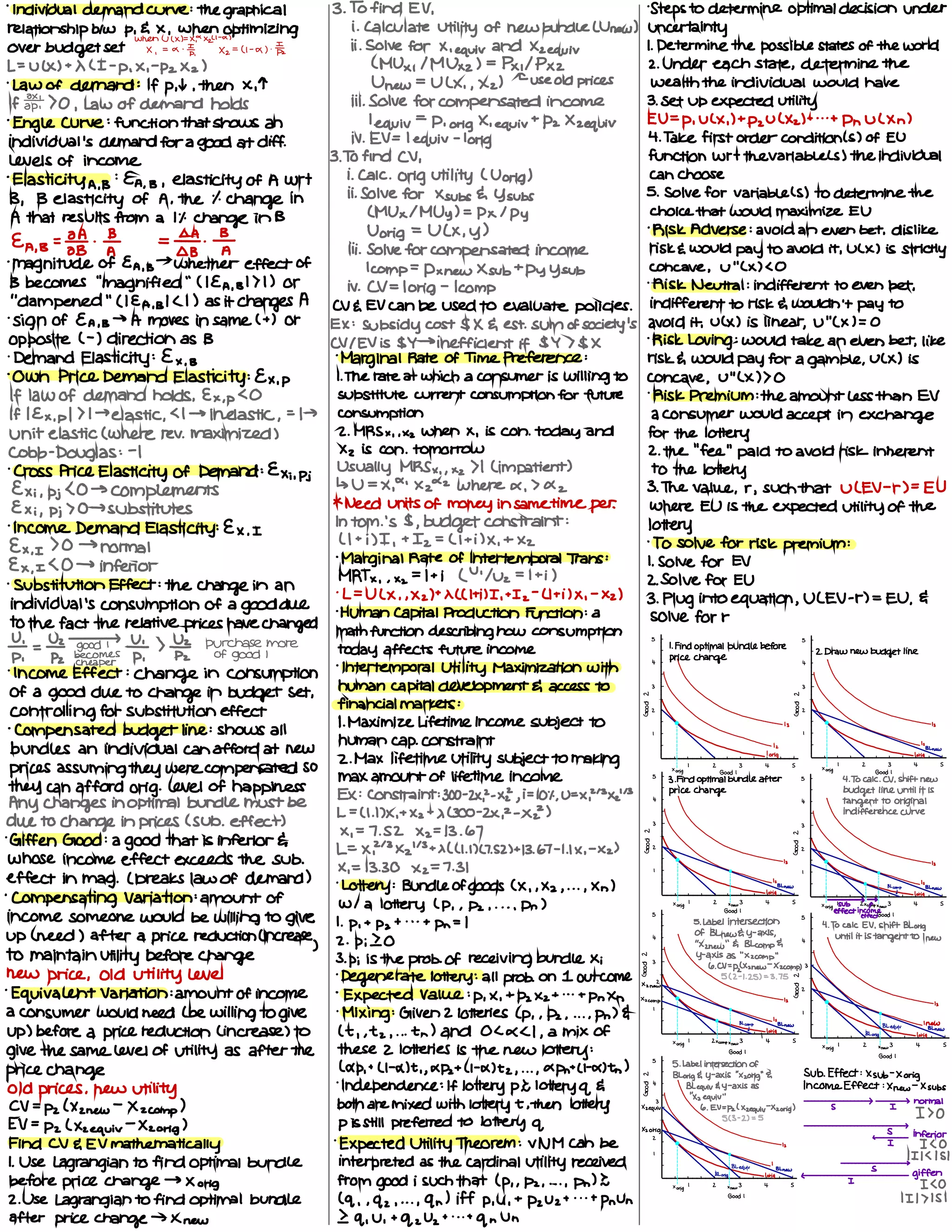
Individual demand curve :
the graphical 3. To find EV ,
.
Steps to determine optimal decision under
relationship btw p ,
EX ,
when
optimizing
i. Calculate Utility of new bundle Wnew ) uncertainty
When U ( X )=XFXzLl
-
a )
Over
budget set x.
= a.
¥.
×z=u -
as .
¥ ii. Solve for X.
equiv
and Xzequiv I. Determine the possible States of the world
L= ULXITXCI -
pix ,
-
pzxz ) ( Mlk , 1MHz ) =
Pxilpxz 2. Under each state , determine the
-
Law of demand : If p.lv ,
then X. T Uncw =
ULX , ,
Xz )
t
Use Old prices wealth the individual would have
If ¥170 ,
Law of demand holds iii. Solve for compensated income 3. Setup expected utility
.
Engle Curve :
function that shows an
I
equiv =p ,
orig
X.
equivtpzxzequivEU-p.ULX.lt/2zULXzlti..tpnULXn
)
individual 's demand fora good at diff .
iv. EV= I equiv
-
long 4. Take first order conditions ) of EU
Levels of income 3. TO find CV ,
function wrtthevariablels ) the individual
-
Elasticity A. B
:
EA ,
, , elasticity of A Wrt
i. Calc .
Orig utility ( Uorig ) can choose
B ,
B elasticity of A. the f.
change in
ii. Solve for Xsubsdaysubs 5. Solve for variables ) to determine the
A that results from a I 't
change in B t.MU//MUy)=px1py choice that would maximize EU
Uorig =
ULX , y )
-
Risk Adverse : avoid an even bet , dislike
EA ,B=fF3 .
Ben = -
BF iii. Solve for compensated income risk 's would
pay to avoid it ,
ULX ) is strictly
.
magnitude Of Ea , B
→
whether effect Of
lump =
phew Xsubtpyysub concave ,
U'
'
LN LO
B becomes
"
magnified
"
( IEA ,
13171 ) or iv. C ✓ =/ orig
-
lamp
.
Risk Neutral : indifferent to even bet .
"
dampened
"
( IEA ,
BILL ) as it Changes A
CVEEV can be used to evaluate policies .
indifferent to risk da wouldn't pay to
.
sign of EA.rs →
A moves in same l t ) Or Ex :
subsidy cost SIX E. est . sum of society 's avoid it .
UCX ) is linear ,
U'
'
C XI=0
opposite ( -
) direction as B CVIEV is Sly →
inefficient if $4 > SIX
.
Risk Loving : would take an even bet ,
like
-
Demand Elasticity :
Ex , ,
.
Marginal Rate of Time Preference :
risk 's would pay for a gamble ,
ULX ) is
-
Own Price Demand Elasticity :E x. p
1. The rate at which a consumer is willing to concave ,
U'
'
LX ) > O
If law of demand holds ,
Ex ,pL0 substitute current consumption for future
.
Risk Premium : the amount Less than EV
If IEx.pl > I →
elastic ,
< I →
inelastic ,
=l→ consumption a consumer would accept in exchange
unit elastic ( where rev . Maximized ) 2. MRS x. ixz When X ,
is con .
today and for the lottery
Cobb -
Douglas :
-
I Xz is con .
tomorrow 2. the
' '
fee
"
paid to avoid risk inherent
.
Cross Price Elasticity of Demand :
Ex ; ,pj
Usually MRSX . ,xz
> I ( impatient ) to the lottery
Exi , pj
LO →
complements
↳ U=X9 '
XYZ Where a ,
> Az 3. The value ,
r ,
such that ULEV -
r )=EU
Exi , pj > O → substitutes
* Need Units of money insametimeper .
where EU is the expected utility of the
-
Income Demand Elasticity :E x. I
lntom .
's $
, budget constraint :
lottery
E x. I
> O →
normal
( Iti )IitIz= L Iti )XitX2 .
To solve for risk premium :
Ex ,
ISO →
inferior
'
Marginal Rate of Intertemporal Trans :
I. solve for Ev
MRT× , ,×z= Iti (
"
luz =
Iti ) 2. Solve for EU.
Substitution Effect :
the Change in an
.
L=UL× , ,×z)t×uHilI ,
+
Iz
-
Lltilx ,
-
Xz ) 3. plug into equation ,
ULEV -
r )=EU .
E
individual 'S consumption Of a
good due
.
Human capital production Function : a
solve for r
to the fact the relative prices have Changed math function describing how consumption
U , Uz ) U ,
s -
s -
-
= -
good I
pm,
) ¥22 Purchase more
today affects future income .
1. Find optimal bundle before
.
z Draw new
budget line
p , pz
becomes of good 1
price change
cheaper -
Intertemporal Utility Maximization with
" -
" -
.
Income Effect :
change in consumption -
-
human capital development 's access to s -
s -
Of a good due to
change in budget set ,
n n
controlling for substitution effect
financial markets :
go , go ,
-1€,
-
Compensated budget line : shows all
1. Maximize Lifetime Income subject to
,
:
y
, .
,
:
y
↳
bundles an individual can afford at new
human cap . constraint .
, .
.
2. Max lifetime Utility subject to
making
. i . . i . . .
orig . .
. i . . i . .
loris. .
I 2 3 4 S I 2 3 4 S
prices assuming they were compensated SO rig good , rig Good '
Max amount Of lifetime income s -
3. Find optimal bundle after s -
4. To calc . W .
shift new
they can afford Orig . level Of happiness
Ex : constraint :
zoo -2×12×22 ,
i 10%0=+1213×2113
-
price change
-
budget line until it is
Any changes in optimal bundle must be
4 -
4 -
tangent to original
L =
( 1. 1) X. t Xztx ( 300-2×12 -
X } ) -
- indifference curve
due to
change in prices C Sub .
effect ) s -
s -
X. =
7.52×2=13.67 N
N
.
Giffen Good :
a good that is inferior 's o
-
o
-
f- X ,
"3Xz"3tX( ( 1.174.523+13.67 -
I. IX ,
-
Xz )
802! 802-•
ewtiescincmmag
.EE#Es9Fwdo:tYumsan3nx.=issoxz=isi
.
.
Lottery : Bundle of goods ( X , ,Xz ,
. . .
,
Xn )
-
I
-
• -
Bhim
.
I I I I l
-
l l
toricI I
, , , ,
I, ,
I
, orig , ,
-
Compensating Variation :
amount Of
w/ a lottery ( p , , pz ,
. . .
, pm ) rig
' Z
gig?
" s
n
.ge#ebcti3eIIgIEIew3
4 s
income someone would be willing to give
s -
s -
Good '
I .
p ,
t
pzt
. . .
t
pm =/ -
5. Label intersection
.
4. To calc EV ,
shift Blorig
Up ( need ) after a price reduction ( increase
,
z .
pizo
4 -
Of BLUEY -
axis ,
4 .
until itistangenttolnew
.
"
Xznew
"
G Blcompda
to maintain Utility before change y-axis as
"
xzcomp
"
-
3.
pi is the prob . of receiving bundle Xi , -
6.
CV=p{
Xznew
-
Xzcomp ) 3
-
new price ,
Old utility Level .
Degenerate lottery : all prob .
on I outcome
o -
512-1.25=3.75 -
-
.
equivalent variation : amount of income
.
expected value :p ,×,+pz×z+
. . .
+
pn× ,
I÷÷u¥•§↳;§o,
.§ ,a consumer would need ( be willing to give
.
Mixing :
Given 2 lotteries Lp , , Pz ,
. . .
. pm ) E =
i -
a
-
•
I Blcoymp
-
IBLequiv
I new
Up ) before a price reduction ( increase ) to ( t , ,tz ,
. .
.tn ) and OLXLI ,
a MIX Of . . . . . .
Kris. .
, , .
Kori. ,
iorig.
?rig
I
Zxcompxnew
} 4 S
I 2
=
3 4 S
give the same level of utility as after the these 2 lotteries is the new
lottery
:
good ,
rig
yoga,
S -
5. Label intersection of
> rice
change
( AP .tl/-X)ti,XPztll-X)t2 ,
. . .
, April ' -
d) th )
n
-
Blom .gg y-axis
"
xzorig
"
's Sub .
Effect :X sub
-
Xorig/
Old prices ,
new utility
.
Independence : If lottery PI lottery q E I
" -
Bleauivday -
axis as Income Effect :X new
-
Xsubs
or -
"
Xz equiv
' '
CV=pz( Xznew
-
Xzcomp ) both are Mixed with lottery tither lottery
xzeausi-6.eu-pzlxzeauiu-xzon.gl
s I
2178
p is still preferred to lottery q
- Scs -23 .
-
s
EV =
Pz (
Xzequiv
-
Xzorig ) xzorig -
Find CVEEV mathematically
.
Expected Utility Theorem : VNM Can be
2
,
;
¥
,
Yg ,
1. Use Lagrangian to find optimal bundle interpreted as the cardinal Utility received .
Iaea
"
s
>
i i ,
Phon, ,
Iorio, , ( giffen
before price change
→ X
orig
from good I such that ( p , , Pz ,
. . .
, Pm ) I
rig
, z
Inns4 s
I
ICO
2. Use Lagrangian to find optimal bundle ( q , ,qz ,
. . .
, qn ) Iff p . U , tpzuzt
. . .
tpnun
Good '
III > 151
after price change → Knew Iq ,
U , tqzuzt
. . .
tqnvn

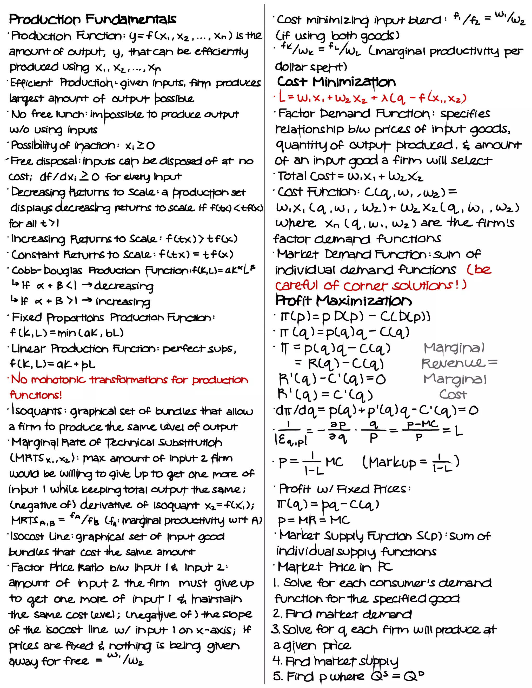
3. Production Fundamentals
'
Cost minimizing input blend :
f '
Az =
W'
lwz
'
Production Function :
y
= f CX . , Xz ,
. . .
,
Xn ) is the ( if using both goods )
amount of output , y ,
that can be
efficiently .tk/Wk=f4WL L
marginal productivity per
produced using X . . Xz ,
. . .
,
Xn dollar spent )
.
Efficient Production :
given inputs ,
firm produces Cost Minimization
largest amount of output possible
.
L =
W , X ,
t
Wz Xz t X ( q
-
f- LX , ,
Xz )
.
NO free lunch :
impossible to produce output
-
Factor Demand Function :
specifies
w/o using inputs relationship btw
prices of input goods ,
'
Possibility of inaction :
Xi 20 quantity of output produced . E amount
'
Free disposal :
inputs can be disposed of at no Of an input good a firm will select
cost ; dfldxi O for every input
.
Total Cost =
w , X , t Wzxz
.
Decreasing Returns to scale :
a production set
.
Cost Function :
Clq ,
w , , wz ) =
displays decreasing returns to scale if fctxlctfcx ) W , X ,
( q .
W , ,
Wz ) t Wz Xz ( q ,
w , ,
Wz )
for all t 71 Where Xn ( q . W .
,
Wz ) are the firm 'S
.
Increasing Returns to Scale :
f Ctx ) > tf Cx ) factor demand functions
.
Constant Returns to Scale : f Lt X ) =
tf Cx )
.
Market Demand Function :
sum of
'
Cobb -
Douglas Production Function : FCK ,
L ) = aka L
's
individual demand functions ( be
↳
If a t BC I →
decreasing careful of corner solutions ! )
↳ If a t B > I →
increasing Profit Maximization
-
Fixed Proportions Production Function :
.
IT L p ) =p Dcp ) -
C L Dcp ) )
f Lk ,
L ) =
min Lak ,
BL )
.
IT ( q )
=p L q ) q
-
C Cq )
.
Linear Production Function :
perfect subs ,
'
IT =p ( q )
q
-
C Cq ) Marginal
f- C K ,
L ) =
a K t
BL
=
Req ) -
C C q ) Revenue =
.
No monotonic transformations for production R
'
( q ) -
C
'
( 91=0 Marginal
functions ! R
'
( q ) =
C
'
(
q ) Cost
.
15090 ants :
graphical set of bundles that allow
.
DIT 1dg =p C q ) t
p
'
( q )
q
-
C
'
( q ) =
O
a firm to produce the same level of output
.
Marginal Rate of Technical substitution
'
lE÷pI=
-
¥
-
To =
=L
( MRTS × , , xz ) :
Max amount of input 2 firm .
p =
MC ( Markup
=
¥ )
would be willing to give up to get one more of
input I while
keeping total output the same ;
.
Profit w/ Fixed Prices :
(
negative of ) derivative of
isoquant Xz=fCx ,
) ; IT L q ) =
pq
-
C Cq )
MRTS a , B
=
fa
HB Lfa:
marginal productivity Wrt
Al p = MR = MC
.
ISO cost Line :
graphical set of input good
'
Market Supply Function Scp ) :
sum of
bundles that cost the same amount individual supply functions
.
Factor Price Ratio btw Input I da Input 2 :
.
Market Price in PC
amount of input 2 the firm must give up
1
.
Solve for each consumer 's demand
to
get one more of input I I maintain function for the specified good
the same cost level ; L
negative of ) the slope 2 .
Find market demand
of the boost line w/ input I on x
-
axis ;
if 3. Solve for q each firm will produce at
prices are fixed da
nothing is
being given a given price
away for free =
w '
lwz 4 . Find market supply
5 . Find p where Qs =
QD

4. .
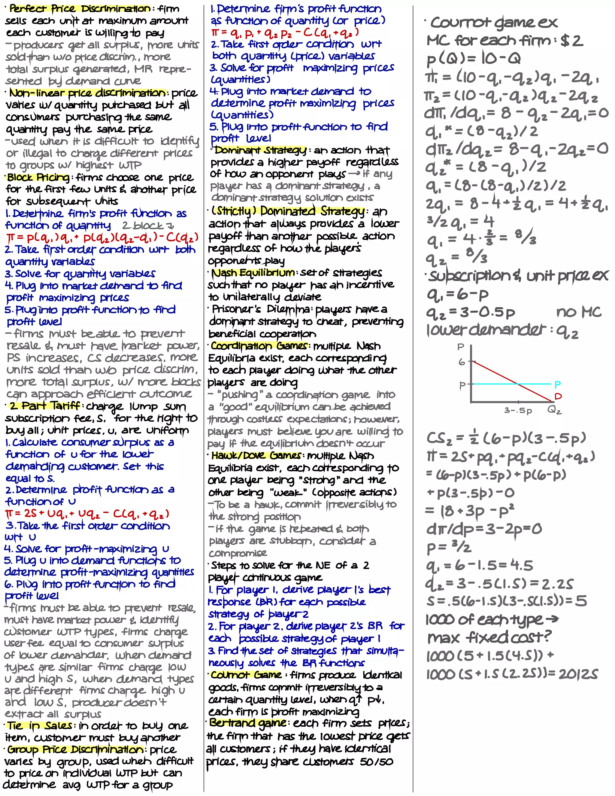
Der feet Price Discrimination : firm 1. Determine firm 's profit function
sells each unit at maximum amount as function of quantity Cor price ) .
Cournot game ex
each customer is willing to pay IT =
q , p ,
t
qzpz
-
C ( q ,
t
ga )
-
producers get all surplus ,
more units 2. Take first order condition Wrt
MC for each firm :
$2
sold than w/o price disc rim .
,
more both quantity L price ) variables
p ( Q ) = 10 -
Q
total surplus generated ,
MR re pre
- 3 .
Solve for profit maximizing prices
sent ed by demand curve L quantities ) IT ,
= ( 10 -
q ,
-
q z
) q ,
-
29 ,
.
Non -
linear price discrimination :
price
4 .
Plug into market demand to
IT z
=
( 10 -
q ,
-
q z
) q z
-
Zqz
varies w/ quantity purchased but all determine profit maximizing prices
consumers purchasing the same low anti ties ) DIT , 1dg ,
=
8 -
of z
-
2g ,
= O
quantity pay the same price
5 . Plug into profit function to find
q ,
*
= ( q .
q y , 2
-
used when it is difficult to identify profit Level 2
or illegal to
charge different prices
'
Dominant Strategy :
an action that ditz ldqz = 8 -
q ,
-
292=0
to groups w/ highest WTP provides a higher payoff regardless
qz* , L q -
q ,
) , z
-
Block Pricing : firms choose one
price
Of how an opponent plays
→ if any
for the first few units E another price player has a dominant strategy , a
q ,
=
( 8 -
L 8 -
q ,
) 12 ) 12
for subsequent units
dominant strategy solution exists
zq ,
=
q -
4 +I q ,
=
4+ I q ,
1. Determine firm 's profit function as
.
l Strictly ) Dominated Strategy :
an
function of quantity 2 block a action that always provides a lower 3/2 q ,
T
4
IT pl of ,
) q ,
t
plqz ) ( q z
-
q ,
) -
C ( q z
) payoff than another possible action
q ,
= 4 .
I =
8/3
2. Take first order condition Wrt both regardless of how the player 's
quantity variables opponents play q z
= 8/3
3. Solve for quantity variables
.
Nash Equilibrium : set of
strategies .
Subscription G unit price EX
4. Plug into market demand to find Such that no
player has an incentive
profit maximizing prices to unilaterally deviate 9 ,
=
6 -
p
S .
Plug into profit function to find
.
Prisoner 's Dilemma :
players have a
q z
=3 -
O . 5 p no MC
profit level dominant Strategy to cheat , preventing
-
firms must be able to prevent beneficial cooperation
lower demander :
q z
resale G must have market power ,
.
Coordination Games :
multiple Nash p
PS increases ,
CS decreases .
more Equilibria exist ,
each corresponding 6 -
units sold than w/o price disc rim ,
to each player doing what the other
more total surplus ,
W/ more blocks players are doing p
-
p
can approach efficient outcome -
"
pushing
"
a coordination game into D
.
2 Part Tariff :
charge lump sum a
' '
good
"
equilibrium can be achieved 3- .
's p
Q ,
subscription fee ,
S ,
for the
right to through costless expectations ; however ,
buy all ; unit prices ,
u ,
are uniform
players must believe
you are willing to
CS z
= I ( 6 -
p ) ( 3
-
.
5
p )1. Calculate consumer surplus as a
pay if the equilibrium doesn't occur
function of u for the lower -
Hawk I Dove Games :
multiple Nash IT =
25 t
pg .
t
pqz
-
C Cq , tqz )
demanding customer .
Set this
Equilibria exist ,
each corresponding to
equal to s .
one player being
"
strong
"
and the
=
L 6 -
p ) ( 3- .
Sp ) t
p ( 6 -
D )
2. Determine profit function as a
other being
' '
weak
"
( opposite actions ) t
p ( 3- . Sp )
-
O
function of U -
To be a hawk ,
commit irreversibly to
IT = 25 t
09 ,
t
Uqz
-
C Cq ,
t
q z
) the
strong position
=
I 8 t 3 p
-
P2
3. Take the first order condition -
if the
game is repeated L both d IT Idp =3 -
213=0Wrt U
players are stubborn ,
consider a
4. Solve for profit -
maximizing u p = 3/2
5. Plug U into demand functions to
compromise
.
Steps to solve for the NE of a 2
q ,
= 6 -
I .
5 = 4 .
5
determine profit -
maximizing quantities
player continuous
game
6. Plug into profit function to find
qz =3 -
.
5 ( I .
S ) =
2 .
25
I .
For player I ,
derive player I 's best
profit level
response LBR ) for each possible S =
.
5 ( 6 -
I .
S ) L 3- .
SLI .
S ) ) = 5-
firms must be able to prevent resale .
strategy of
player 2
must have market power E identify 1000 of each type →
customer WTP types ,
firms charge
2 .
For
player 2 .
derive player 2 's BR for
user fee equal to consumer surplus
each possible strategy of player I Max fixed cost ?
of lower demander ,
When demand
3 .
Find the set of
Strategies that Sim Ulta -
1000 ( g + 1. g ( 4. s ) ) +
types are similar firms
charge low newly solves the BR functions
U and high S ,
when demand types
-
Cournot Game :
firms produce identical 1000 ( S t I .
S L 2 .
25 ) ) =
20125
are different firms
charge high u goods ,
firms commit irreversibly to a
and low S , producer doesn't certain quantity level ,
when qt pt ,
extract all surplus
each firm is profit maximizing
.
Tie in Sales : in order to buy one
.
Bertrand game
:
each firm sets prices ;
item ,
customer must buy another the firm that has the lowest price gets
.
Group Price Discrimination :
price all customers ; if they have identical
varies by group ,
used when difficult
prices, they share customers 50150
to price on individual WTP but can
determine avg WTP for a group