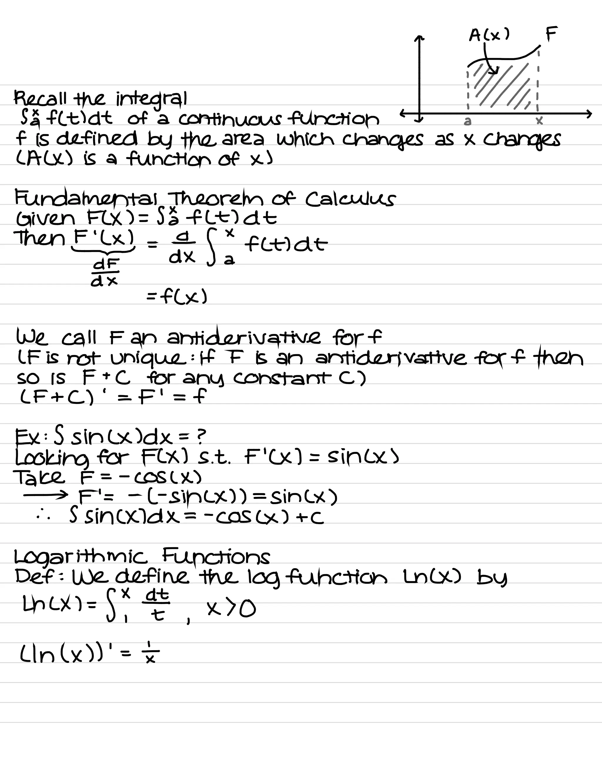
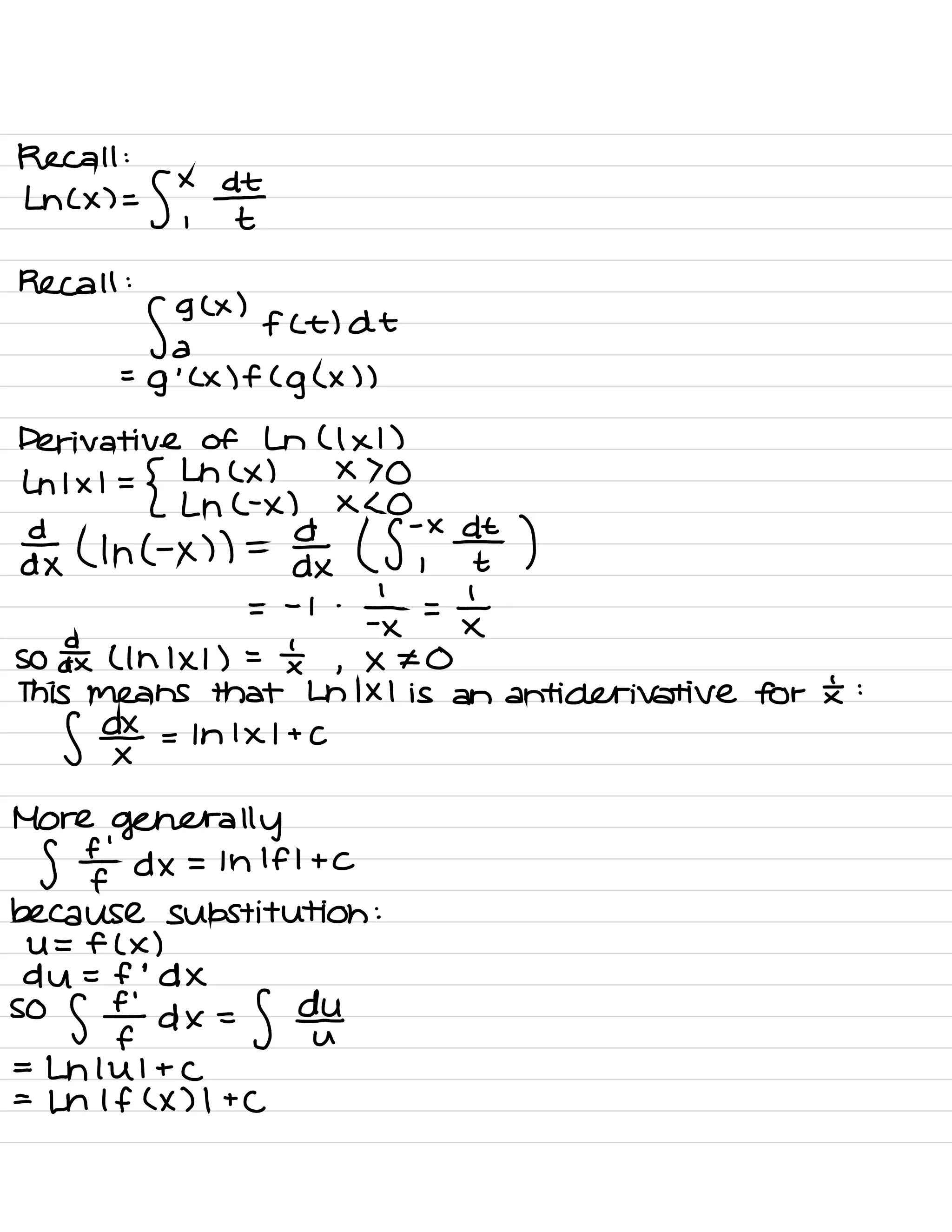
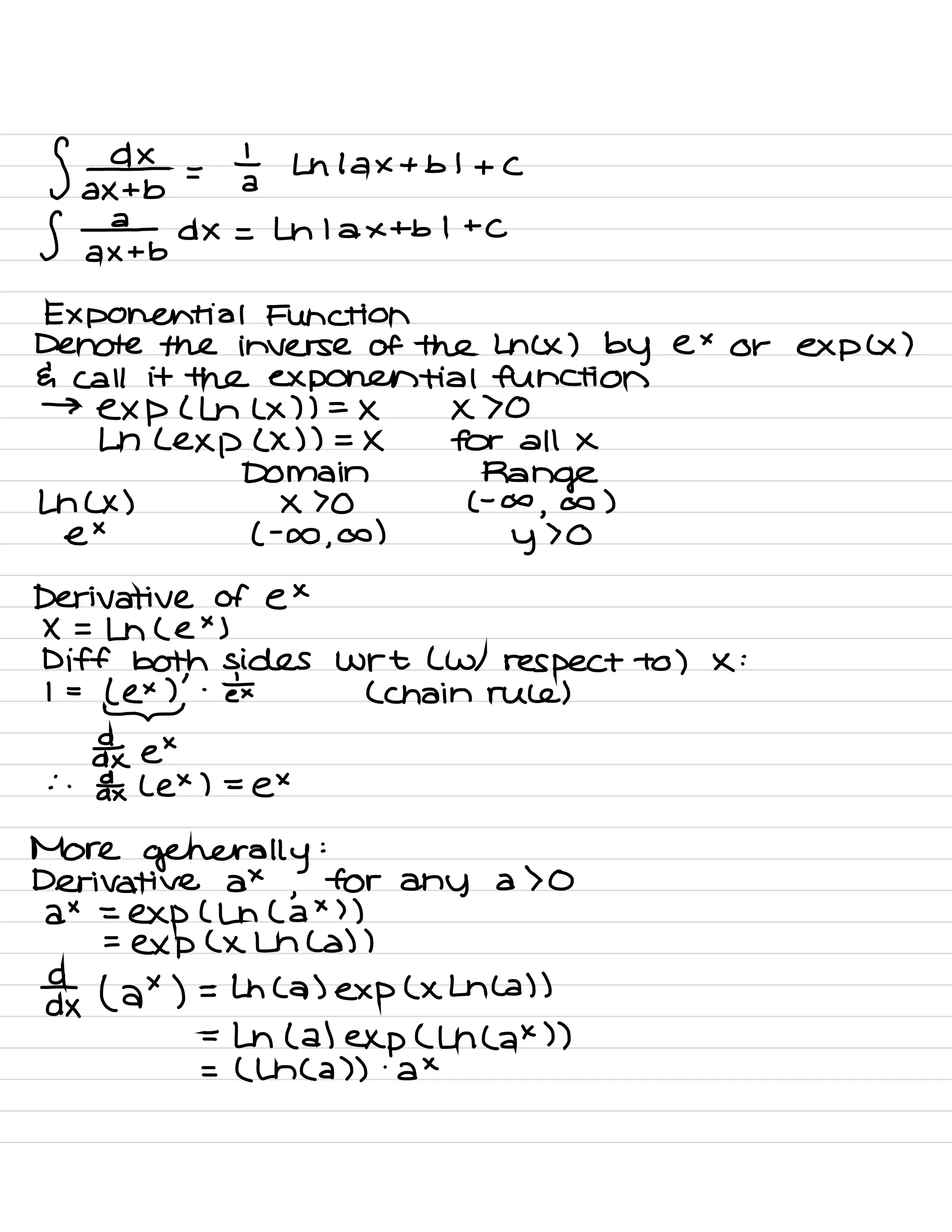
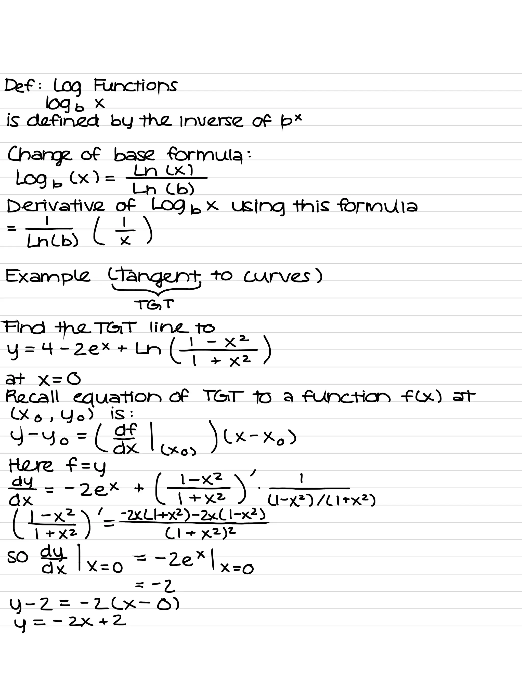
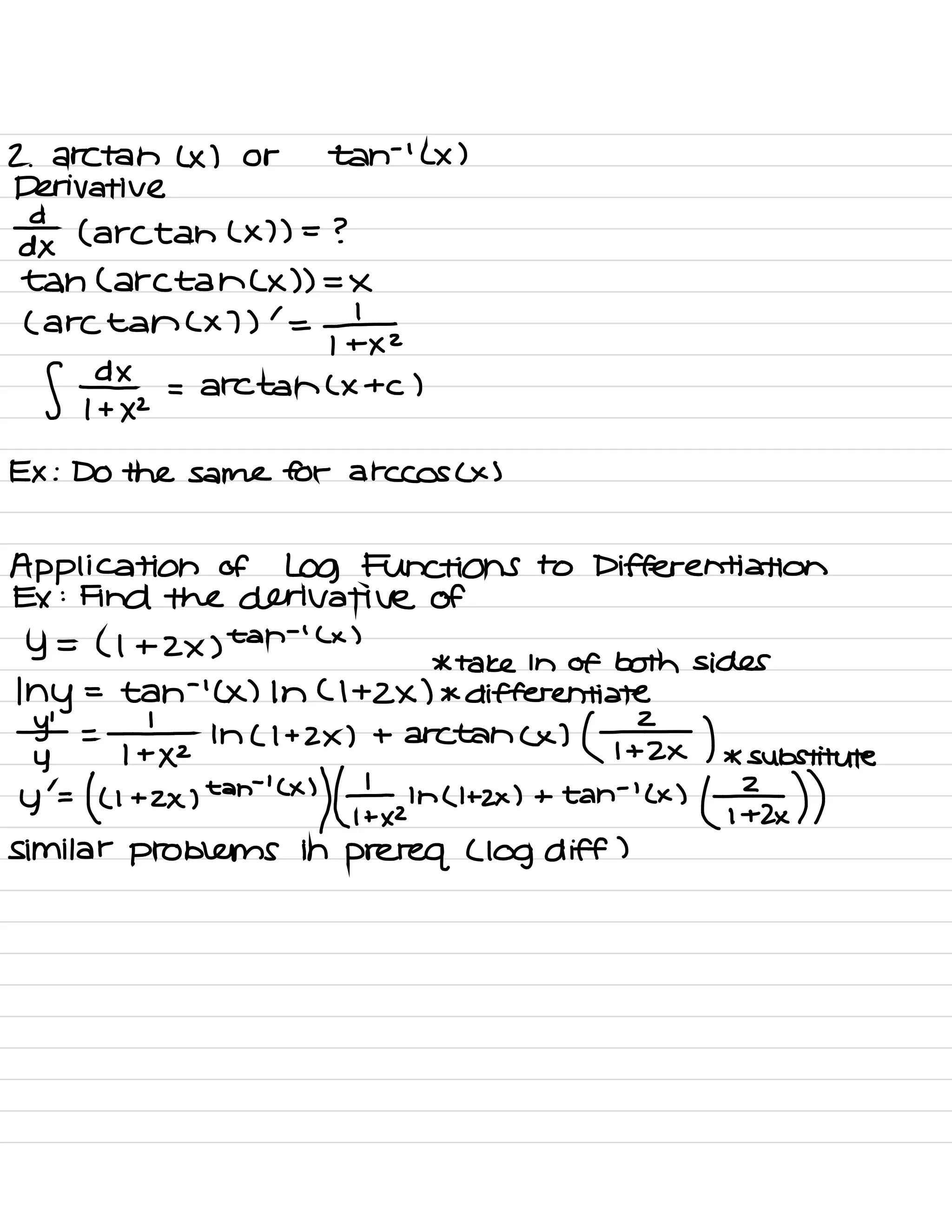
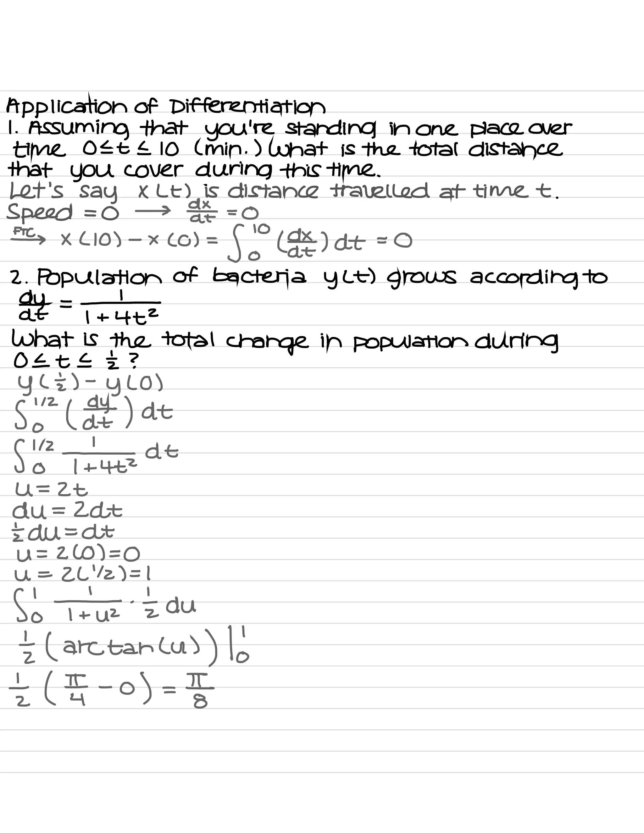
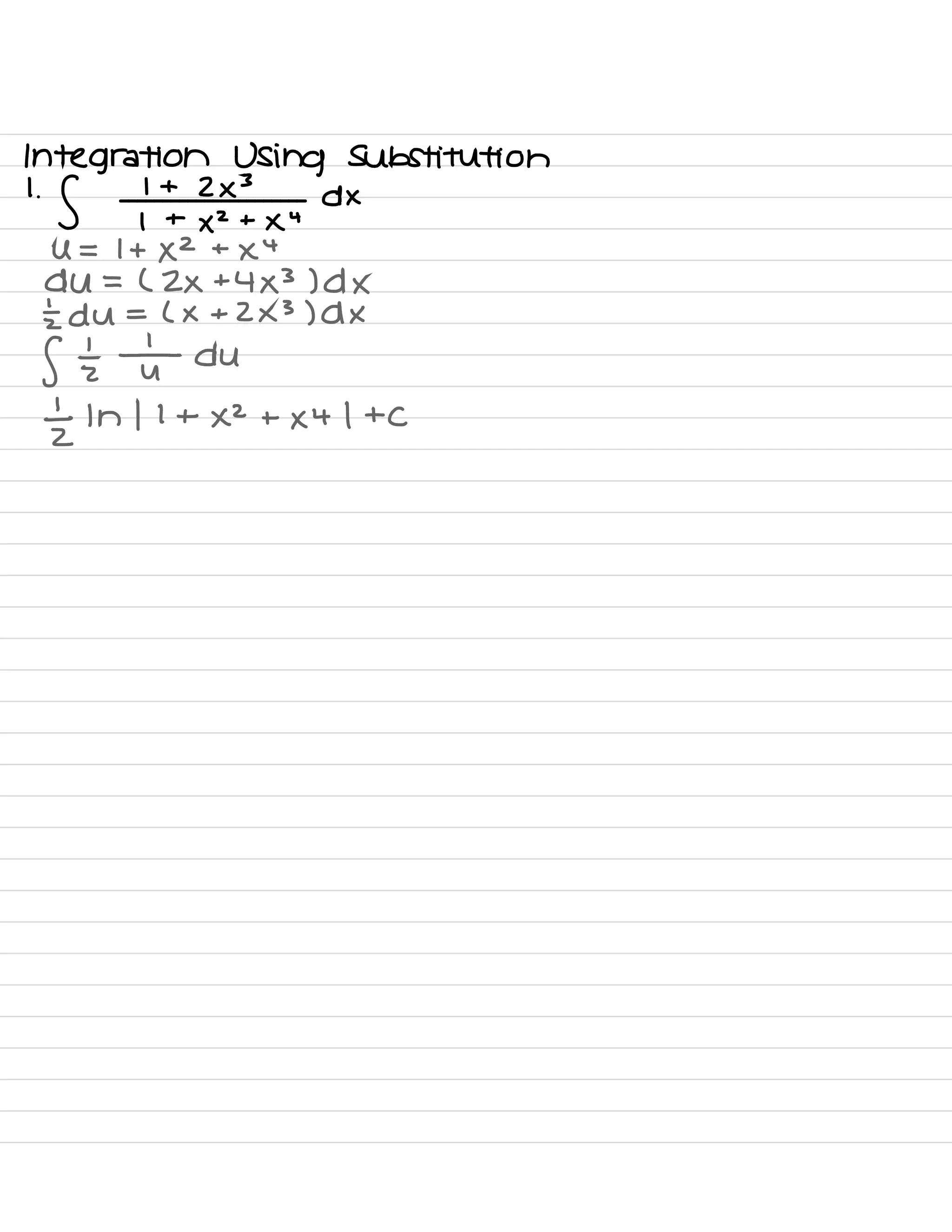
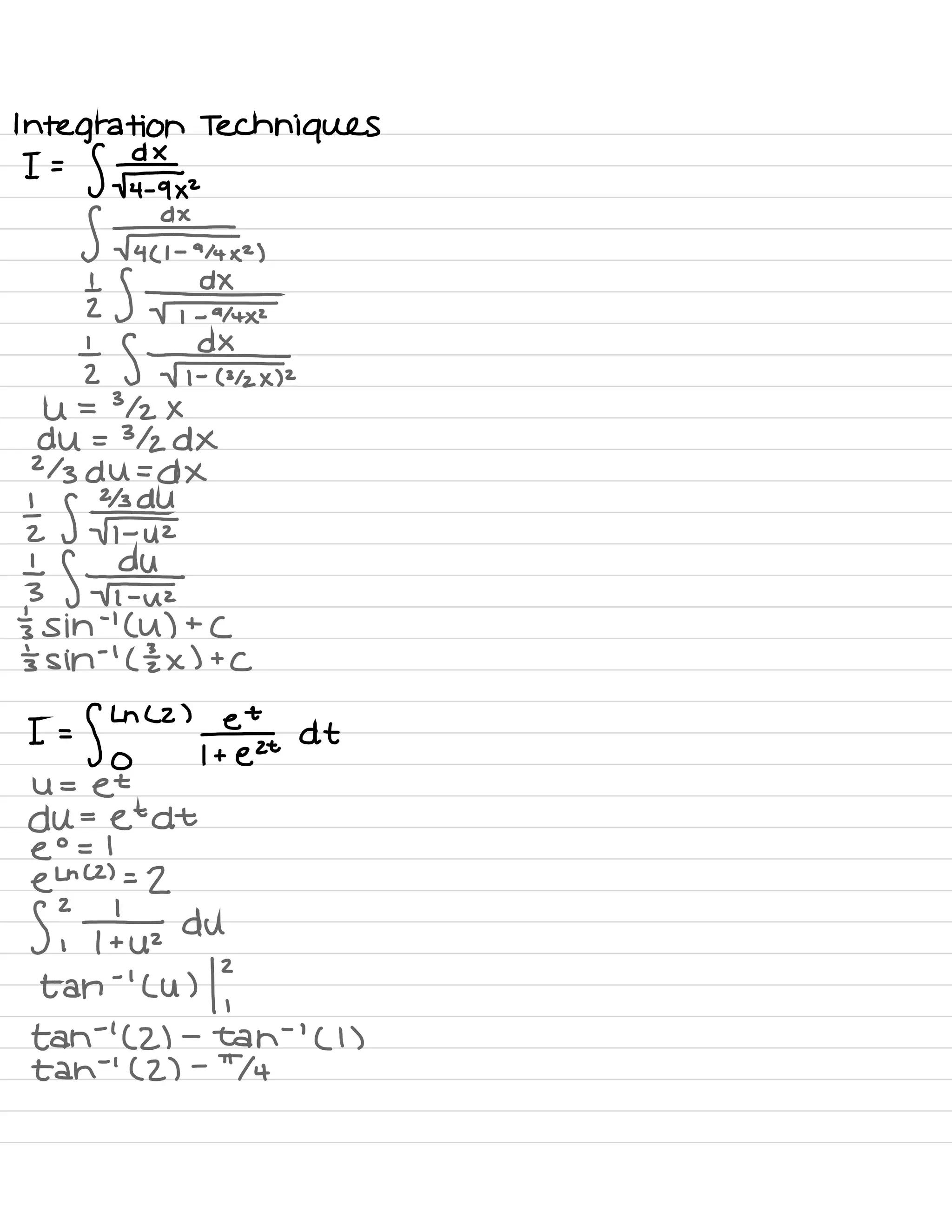
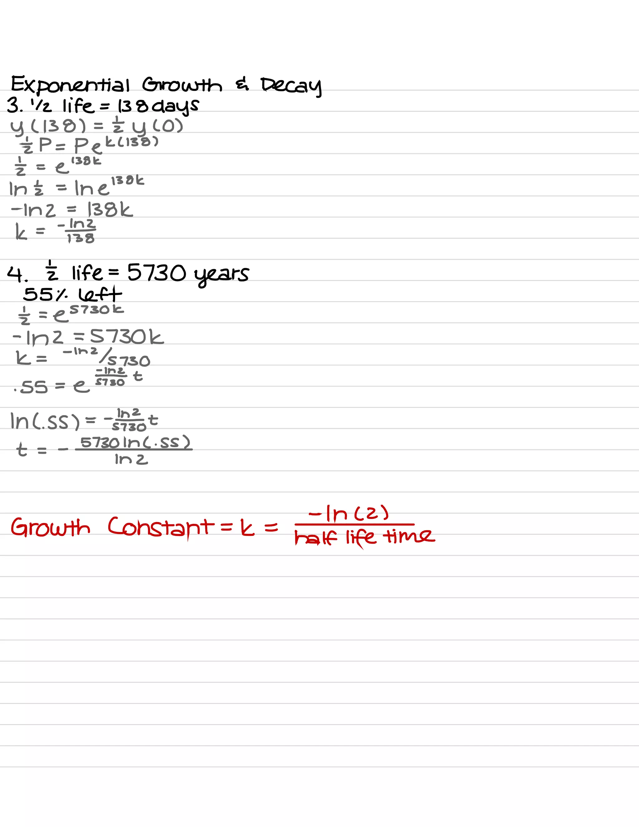
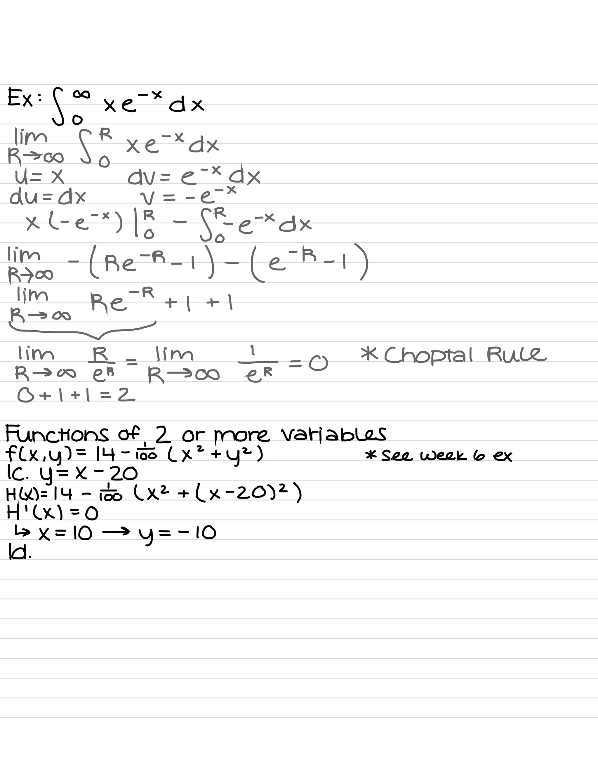
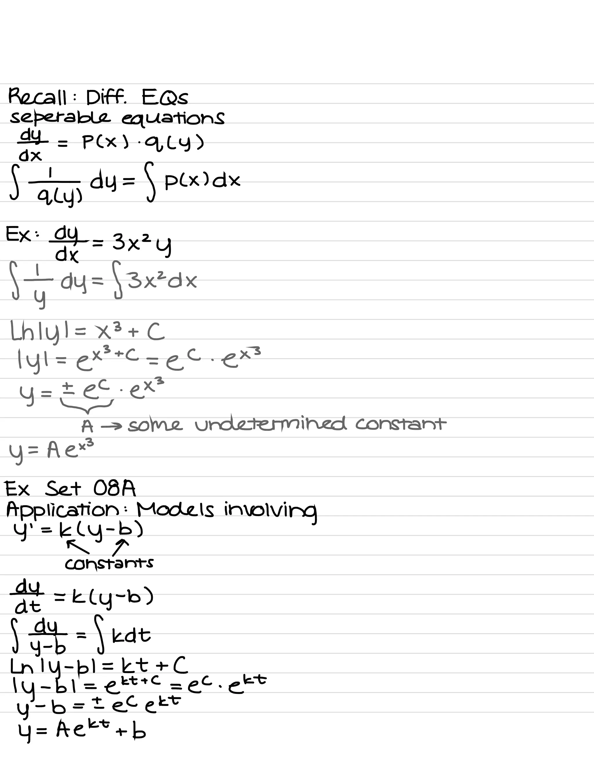
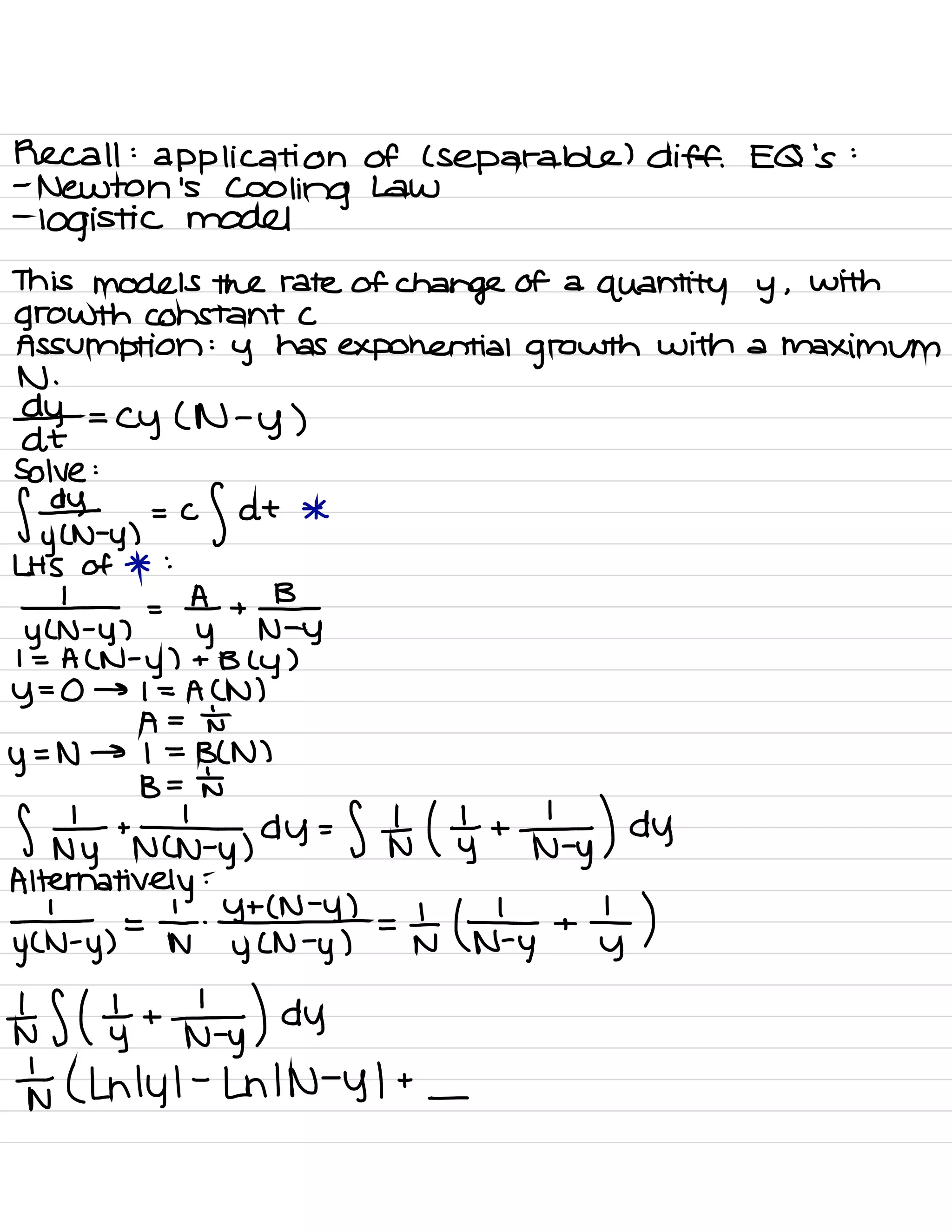
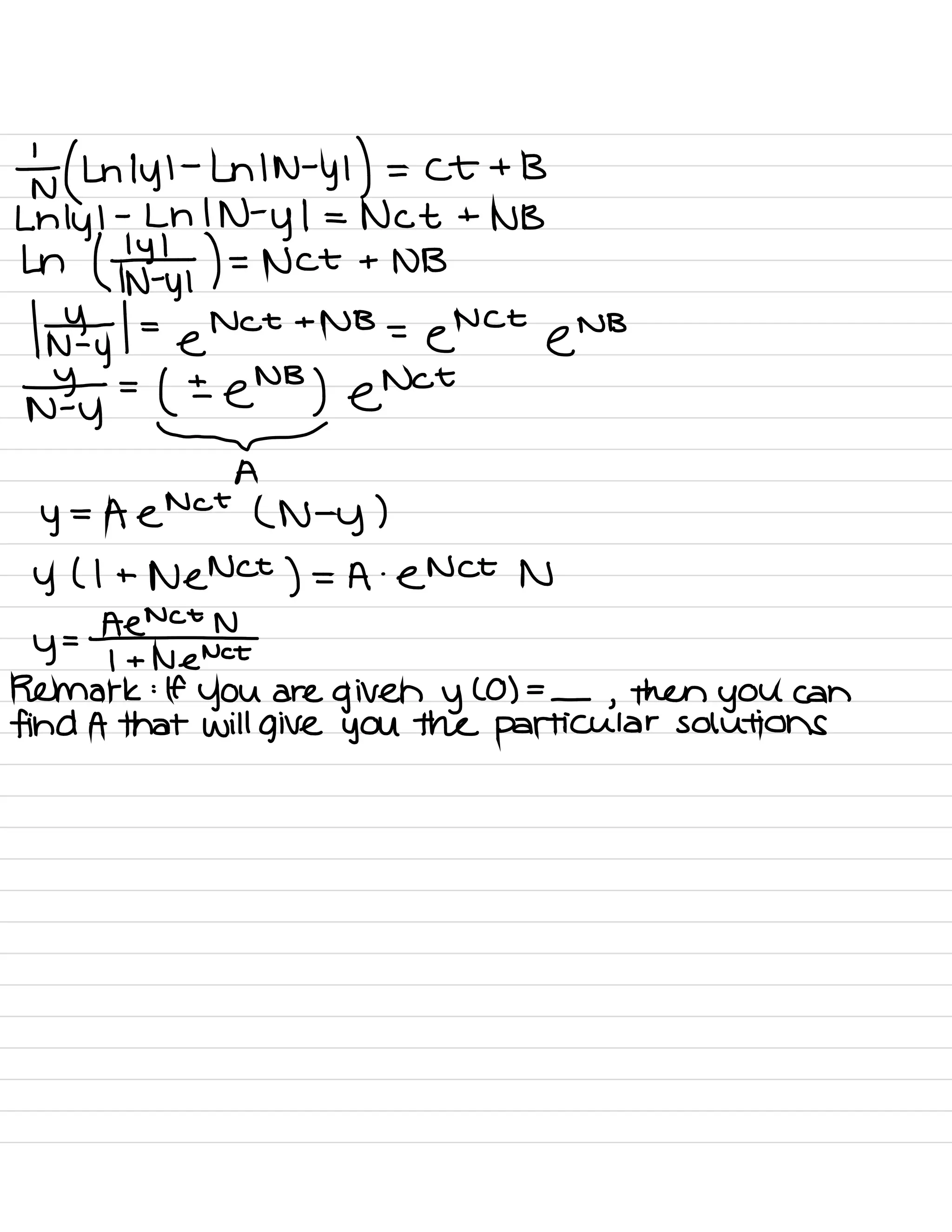
The document covers fundamental concepts of calculus including the definition and properties of integrals, derivatives of various functions such as logarithmic and exponential functions, and applications of integration and differentiation. It also briefly discusses inverse trigonometric functions, exponential growth and decay, as well as applications of integration techniques for calculating volumes and areas. The document includes numerous examples and emphasizes the importance of understanding the relationships between different mathematical functions.

1. Catullus B

2. n A ( x ) F
⇐% '
Recall the integral
i i
I I
SI fltldt of a Continuous function
<
v
a x
>
f is defined by the area which changes as × Changes
( ALX ) is a function of × )
Fundamental Theorem Of Calculus
Given FLX ) = SI flt ) dt
Then
F'L×)_ =
day f I fltldt
⇐
DX
= f ( x )
We call F an anti derivative for f
LF is not unique : if F is an anti derivative for f then
SO is F +
C for any Constant C)
( F + C)
'
= F
'
= f
Ex :S sink )d×= ?
Looking for FCX ) st .
F
'
( × ) = sink )
Take F = -
COS ( × )
→
F
'
=
-
C- sin ( x ) ) =
sin ( × )
.
'
. S sink )d×= -
cos ( × ) + C
Logarithmic Functions
Def :
We define the log function LNLX ) by
Lnlx ) =
Sf aft ,
× > 0
( In ( × ) )
'
=
,÷

3. Recall :
Ln ( x ) =
S ,×
¥
Recall :
gglx
)
f (E) At
a
=
g
'
( × ) f (
g ( × ) )
Derivative of Ln ( 1×1 )
Ln 1×1 =
{
↳ ( x ) × > o
Ln C- x ) × < 0
Fdx ( Inc -
x ) ) =
day ( Sjxdzt )
=
-
i .
÷×=t
SO a£ ( In 1×1 ) =
tx ,
× ¥0
This means that Ln 1×1 is an anti derivative for £ :
f d¥ = In 1×1 + C
More
generally
S ¥ dx = 1h If I + C
because substitution :
U = f ( x )
du = f
'
d X
so
s¥dx= S out
=
Lnlul + C
=
Ln If ( X ) I +
C

4. ) ¥+5 = at Lhlaxtbl + c
) a×÷bd× = Lhlaxtb I +
c
Exponential Function
Denote the inverse of the Lncx ) by e× or exp ( × )
E call it the exponential function
→
exp ( Ln ( × ) ) =
× × > 0
Lh ( exp ( X ) ) = X for all X
Domain Range
Ln ( x ) × > 0 ( -
oo
,
a )
e× ( -
oo .co )
y
> 0
Derivative of ex
X = Ln ( ex )
Diff both sides wrt ( w/ respect to ) X :
1 =
(E)
.
et ( chain rule )
& ex
.
'
.
Fx ( ex ) =
e
×
More
generally
:
Derivative a×
,
for any a > 0
a× =
exp ( Lh ( a
×
) )
=
exp ( × Ln (a) )
otdx ( a× ) = Lh (a) exp ( × Ln (a) )
=
Lh ( a) exp ( Ln ( ax ) )
= ( Lh ( a ) ) .
ax

5. Def :
Log Functions
109 b
×
is defined by the inverse Of b×
Change of base Formula :
69 b
( x ) =
#
Ln ( b )
Derivative of Log bx Using this Formula
=
-1
Lh ( b ) ( I )
Example
MI
to curves )
TGT
Find the TGT line to
y
= 4 -
Zex + Ln
( ¥122 )
at ×=0
Recall equation Of TGT to a function flx ) at
( X o , y o
) is :
y
-
yo =
( If
Here f=y
d×
/
( xo ,
) ( ×
-
Xo )
day =
-
zex +
( ¥1 )
'
'
T.tn ,
( tT# )
'
=
-2×4*2*1
( I +
× 2)
2
so ddhtx |×=o = -
2e×l×=o
=
-
z
y
-
2 = -
2 ( ×
-
o )
y
=
-
2×+2

6. Inverse of Trig Functions
1. arcsin ( x ) Or sin
'
'
( × ) is the inverse of sin ( × )
sink ) ( I ,
1 ) EE ,
-1 )
arcsih ( × ) ( i
,
E) ( -1 ,
-
E)
i¥¥sink ) [ 9¥I,
#
a ]Eating ]
arcs in ( × ) [ -
1
,
1
] [ -
tlz ,
tlz ]
Derivative
ddx ( arcs in ( × ) ) = ?
sin ( arcsin ( × ) )=× by definition
NOW diff both sides :
( arcsin ( × ) )
'
coscarcsinlx ) ) = I ( chain rule )
( Os ( arcsin L × ) ) = Fearon ( x ) )
= -1- ( sihlarcsih ( × ) ) 72
=
#
Why positive ?
range of arcsinlx ) is [ -
72,72 ]
and over E 't
12 ,
172 ] ,
cos is 20 ( positive )
( arcsincx ) )
'
=
-1
. × 2
ftp.xgz-arcsincxstc

7. 2 .
arctan ( × ) or tah
-
'
L × )
Derivative
* ( arctah ( x ) ) =
?
tan ( arctah ( x ) )=×
( arctan ( x ) )
1=11+ ×
2
f My = arctan ( x + c )
EX : Do the same for arcos ( x )
Application of Log Functions to Differentiation
Ex :
Find the derivative of
Y = ( 1 + z× )
tan
- '
( x )
* take In of both sides
lny =
tan
-
'
( x ) In ( I + ZX ) * differentiate
yj
=
¥2 in ( 1+2×1 + arctancx )
( ¥ ) * substitute
y
'
=
(( i + zx )
tank '
) # zlnutzx ) + tan
-
'
L × )
(B) )
similar problems in
prereq ( log diff )

8. Application of Differentiation
1
.
Assuming that you're standing in one place over
time OELE 10 ( min . ) what is the total distance
that you cover during this time .
Let's say × Lt ) is distance travelled at time t .
Speed = 0 → dtae =
0
#s x ( 10 ) -
x ( o ) =
fob (daxz ) At = 0
2. Population of bacteria
y Lt ) grows according to
dY- =
-1
At 1 + 4+2
what is the total
change in population during
0 It E I ?
y ( ÷ ) -
y LO )
Sindh ) at
S
'
oh 147 at
U =
Zt
du = Zdt
Edu = At
U = ZCO ) =
0
U =
2L
'
12 ) = I
Sol ¥ .
tz du
I ( arctancu )
) to
± ( IT -
o
) =
E

9. Integration Using Substitution
1
.
g
1 + 2×3 dx
1 +
×
2 +
×
4
U = It XZ +
×
4
du = ( 2×+4×3 ) d ×
I du = ( × + 2×3 ) d ×
f tz f du
tz In 1 I + ×2 + × 4 I + C

10. Integration Techniques
I =
S¥ra×.
S #4 ( l -
914×2 )
⇒ era
⇒ :* .
U = 3/2 ×
du = 312 DX
213 du =
DX
{ gear
→
a *
's sin
-
'
( U ) +
(
's sin
-
'
( I x ) t
C
I =
fly
" '
feet at
U =
et
du =
etdt
e
°
= 1
e
Ln (2) =
2
2
S ,
# du
tan
- '
( U ) / ?
tah
-
'
(2) -
tah
-
'
( 1 )
tah
-
'
( 2) -
74

11. Exponential Growth E
Decay
3 .
'
12 life = 138 days
y ( 138 ) = £ y ( 0 )
£ P = pek ( 138 )
£ =
e
1 38k
In tz =
In e
138 k
-
In 2 =
138k
K =
-
1h2138
4 .
tz life =
5730
years
55% left
tz =
e
5730 k
-
In 2 = 5730k
K =
- ' h
2/5730
. SS =
e
¥2 t
In ( SS ) =
is'F÷ot
t =
-
5730 In C. Ss )
In 2
-
In (2)
Growth Constant =
K =
half lifetime

12. Application of Integration :
Area Between Curves
A= 58 ( f ( × ) -
g ( × ) ) dx
A =
Set ( f (
y ) -
g (
y ) ) dy
Ex :
Find the area between y=x3
-
× E y
=3 ×
^
•
×
3 -
× =3 X
•
X
3 -
4× = 0
× ( ×2 -
4) =
0
HX ( x + 2) ( × -
2) =
0
. S -4 ( ×
3 -
×
-
3×1+502 ( 3×-1×3 -
× ) )
S -9 ( x
3 -
4× ) + 502 ( -
× 3+4 × ); ÷, ×4 -
2×2 Kz + -
tax
4+2×420
-
(4) (16) +
(2) (4) + ttu ) ( 167+2 (4)
-
4 +
8 -
4 +
8 = 8
Volume of Solids Using Area of Cross Sections
LW =
A .
ax
→
V e
E A
.
ax
a E × Eb
→
V =LFo ( [ A .
A X )
Assume :
A is only a function Of ×
V =
Sba Ak ) dx

13. Ex :
zn
Find the volume Using vertical
• 4
cross sections perpendicular to
× -
axis
" '
% ,
•
2 Y
> LW = ( Ih( × ) .
y ) .
ax
L7 -
3 • At A
×
l
na
,
Need to find h G y in terms of × :
h ( x )
A''
s ,
Y
:
y^z
( 0,2 )
v
17< >
ax
y < >
✓
3
×
( 3,0 )
Slope :
-
2/3
y
-
0=-43
( ×
-
3)
YI-
2/3 X +2
h : 4 ( 0,4 )
3
s x
✓
z ( 3,0 )
Slope :
-
413
z -
0 = -
413 ( ×
-
3)
z =
-413×+4 c- h( X )
V=
'zf3o ( 81A ) ( ×
-
3) 2dx

14. Recall :
Volume of Solids
2^4
IV =
£ (
B.
h ) ( Ox )
^ "
1
,
h|% v =
IS ? ( Bxh ) dx
a
2 Y
✓
c-
Fox
XLz
0×
b
2
r
h :
4
^
h ( × ) =z(× )
*✓
~
3
s ×
= -
413 ( X -
3)
B : Y ^
2 BCX ) =
y ( X )
BUY>
×
= -
2/3 ( ×
-
3 )
v 3
Example
Solid whose base is the region bounded by
y=×3 n
2
y
= 8
y
-
axis 8 y
1 >
Find the volume when the
'
cross section perpendicularX /
u /
to the y
-
axis is :
t
(a) square
÷g¥%yk%.→.
,
II.ftp.sargsssection

15. xy
-
plane
Y^
8 - - -
Ty
=×3
*.
< s
X (
y
) =y"
3
=B( y )
✓
x V=S°8 y "3dy
b)
rectangle of height Ty
#
ry
#
×
I area of Cross section =×Vy
f
V=So8(×Vy)dy
- Day
C) semicircle
area of Cross section =
'ztr2
F#y
=
'zt( E)
2
g- goy
V=tzTSo8¥dy=÷o # 5084213dg
IB
Density
Case 1 : Linear Density
Consider the rod with density P that is constant
along each vertical cross section G
)( '
'
) changes continuously'
→ P is a continuous function OTX
yro×~P
a LM= mass of a small slice
a AI H =e( × ) .
ax
( l I 1 ) - -
v a ×
bxdensity length

16. Total Mass = M
a E e ( × ) .
Llx
a Ex I b
As a × → 0 : M = Sba e ( × ) dx
Def : We call @ ( × ) the linear mass density function .
Example :
Find the total mass of 5 meter rod with
@ ( × ) = I
0£ x ± s
( l + ex )
2
M=
f so
¥7,2 dx
Case 2 :
radial density
Disk of radius R with density e :
-
function of radius
-
E
-
changes continuously
.
g¥=f⇐r
Mass of Small Strips :
4Mt ( Ztr .
Ar )
M = Zt for ( r .
e ( r )
)dr
Def :
C ( r ) is called radial density function
Example :
The population in a
city is distributed
accordingto the density function :
P ( r ) = 8-0
01 re 3
9 + r2
Find the total population
M=
Ztf 30 Lr .
a8¥rz ) dr
= 80 ITS } {+4-2 dr

17. Def :
Average of
,
a continuous function over [ a
,
b ] :
b -
a
fab f
MVT :
f ( c) ( b
-
a) =
S by f
f ( C ) =
1
f by f
b -
a
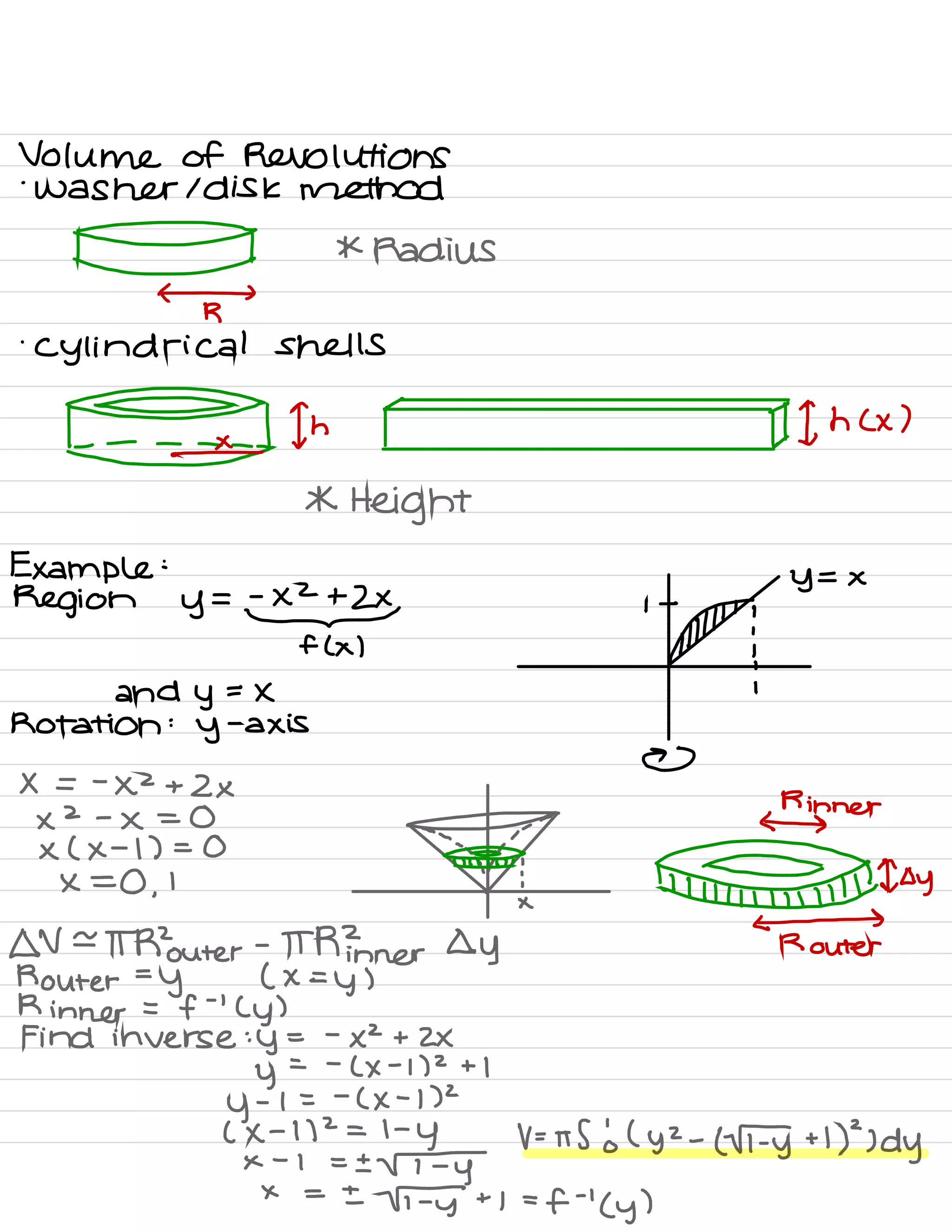
Volumes of Revolution
Disk 1 Washer Method
f
Yn
,
Rotate the region given by
- - -
#
y=f(× ) over [ a
,
b ] E.
a<
trdhEtffD
'
Ina+EYoiImeof small slices
✓
EH =
II.
Iravecitrz
) -
ax
⇒
What is R ?
R = fc × )
LW =
( IT ( f ( × ) ) 2) .
<×
Ve E ( IT ( f ( × ) )2 ) .
DX a E X E b
V =
S ba IT ( f L × ) )2d× = IT
fba Lf(×D2d×

18. Washer
n flxl Rotate the region bounded
Y
-
by y=fC× ) , y=g ( x ) over
nigcx)
I
[ a ,b ] along × -
axis .
' ' '
<
&y¥÷ppµ§}
what is the volume ?
v
- fix
,E#µff
tratertrinner
g ( × )
small volume
-
area of cross section .
DX
=
#Router
2 -
TR
inner
2) DX
V = IT fab #( x ) )2 -
( g ( × ) )2) DX
We Can similarly find volumes of revolutions if the
rotation axis is the
y
-
axis or x=a ( vertical lines )
Or y=b
Example :
region bounded by y=4 -
×2 and ×
-
axis
^
4
and y
-
axis
m )
v 2 ×
Find the volume when axis of revolution is :
(a) the X
-
axis .
LW _~(#R2 ) DX
ftp.tlff# FR = it ( 4- xztax
If V =tf2o ( 4- ×2)2d×

19. b) the line
y=
-
l
'
⇐
ftp.t#=ffMtrou+eruin
.
⇒
V= IT
fo2 ( ( flx ) +112 -
(1) 2) dx
V= IT f2o ( ( S + x2)2 -
1) dx
=
If } 25+10×2 +
×4
-
ldx
: IT
f2o
X
"
+ 10×2+24 DX
= it
( st ×
5
+
If ×
3+24×1/20
= IT ( 325 +
3k + 48 )
V =
fab ( HR2ou+er
-
HRZ
inner
)d×
C) × =3
#
V= IT
504132
.
( 3 -
f-
'
( y )12 ) dy
##_#i#
Find f- '
(
y ) :
f-
'
C
y )
, y =f( × ) = 4 -
×2
3
X 2=4 -
y
ginner ×=±Fiy
Efi IQY
f- '
C
y ) =
Fy
e-
Router

20. Cylindrical Shells Method
, :#⇒ ,
.is#y.t=l-=====I-
*
-
a
¥-7,
ou
= I→nI
.
IIt < >
c- ZTR
R
Volume of shell :
OV e ( ZTR ) .
h .
DX
R ( × ) = ×
h ( × ) =f ( × )
V =
Zit Sab X. f ( × ) dx
Remark :
Similarly for when the axis of rotation is
-
×
.
axis
-
×=a
-
y
=
b

21. Example
:
Region :
y = 4 -
×
2
×
-
axis
4
h¥¥EIH#€ .
tea
3 R ( × ) o
#
a
n
; I
<
ZTR
>
hlx ) = f ( × )
R ( x )
=3-
×
DV a
21T ( 3 -
× ) .
f ( × ) -
4 ×
V = Zit
f 20 ( 3 -
X ) f- ( X ) DX
= ZT
f 20 ( 3 -
× ) ( 4 -
× 2) dx

22. Volume of Revolutions
.
Washer / disk method
⇐ * Radius
<
R
.
Cylindrical shells
*
-
InTthcx )
=¥ ,
*
Height
Example :
Region y=-×2+2×_
i.ph;
Y=×
f ( × )
and y
= X
I
Rotation :
y
-
axis
•
× =
-
XZ + Zx
x2 -
×=O
==
Inner
× ( x
-
1) =O
I#¥T
-
x=O ,
1 ,
Fit 'I0Yx -
-
0VeTR2ou+er -
TR ?nner Lly Router
Router =y ( x=y )
Rinner = f.
'
(
y
)
Find inverse :y=
-
×2 + Zx
y
= -
( ×
-
1) 2+1
y
- 1 =
-
( ×
-
1)
2
( × -
1) 2=1 -
Y V= it S 'o( yz -
try +
1) 2) dyx
-
i =
try
× =
Iffy +1 =
f-
'
( y
)

23. Application of Integration : Work
Work = force x
displacement
When force is only given by gravity ,
then
Force = mass ×
acceleration
e
10
F =
m
.
g
m = Mass =
density ×
length
:-
linear density
( like rod )
Example :
100 meter chain attached to a 300 meter
building
G chain has
weight =
300kg
HOW much Work is done when chain is lifted to
the top ? ( chain has uniform density )
^
^
Ioy { ✓
loom
OW e
( force ) ×
displacement
y
. - - - -
-
y 30L F
F =
mass
.
g
v v
Density =
300 ÷
100=3
Mass = 3
'
length
= 3 '
ay
→ F = ( 3.
Qy )
.
9 g
=
10
F = 30 .
ay
QW ±
( 30 .
ay ) .
y
→
W =
flow ( 30 .
y ) dy

24. HOW much force is done to pull half of the chain to
the top ?
^ For the top half :^
} 100 m
W+op half
=
580 ( 30 .
y ) dy
300
V
m
y
* For the bottom half :
v v Owe ( 3. Oy
.
g ) .
so
W
bottom half
=
SSF ( 30 ) ( SO
)dy
Wtotal =
Wtop half
+ W bottom half

25. Recall from last time :
Find the Volume of the solid
Obtained by rotating the region
:
y =×
, y
= -
×2+2×
about the
y
-
axis
Can Use the shell method
-
o
#
F¥t
If h
÷ ZIX
: V = ZHS x. hcx )d×
=
ZTSX ( f ( x )
-
g ( X ) )d×
= ZTSX ( -
XZ + Zx -
x ) DX
Y=fC × ) = ¥2
Rinner I
# I Router
× = -
1 a
* a. ox
X
-
axis
, 1 1
11 1 1 11 1 1 1
Y =2
y
-
axis
Iaea.
'
axis of rotation :
y=2
DV a ( IR2ou+er
-
TR Zinner ) DX
Router =
2
R inner
= 2 -
f ( × ) = 2 -
¥2
V =
IT SQ, 22 -
( 2 -
¥ )2d×
#
# YIYTIZYZ . 1 -
( it (E) 2.1 )
ztpf/
V 2
1¥ =
IT ( 4 -
÷ ) =
IT (E)
Vi
Vz =
ZITS in ( 2 -
y ) (
T
-
1)
dy ¥#y
R = 2 -
y
h =
f-
'
( y ) -
( -1 )
h =
yt -
2 +1 =
ty -
1

26. Work :
Ex :
A 10 M Chain with non
-
uniform density
e (
y ) =
e
9
kg / M
0 E
y E 10 ( A )
Q I ) What is the work done for lifting the chain
Straight up so that A is 10 m above ground
n
•
A
"
.
→
.
fyis
EYE.EE#yFehaa9nmgnt
=
mass .
g
✓ A
we
Force e ( C ( y
) .
oy ) .
g
owe ( e (
y ) .
oy
.
10 ) .
y
W =
58 ( e ( y ) .
10 ) .
y dy
=
10 S to EY .
y dy
↳
integration by parts
QZ ) What is the work done if we now lift the
whole chain to the top of the building ?
,
of oyq•fAy→
→
^y
0W=
Erg
.
displacement
e. (
y ) .
oy .
g-10 -
y

27. 21 3 ^
Density of liquid : 500
kg1m3< > ^
Work done to pump all
liquid to 2 m above the
- ^ Opening ?
=
12 (
g= 10 )
6
y I
✓ v
=r ( y )
AW = Force .
Displacement
F = mass
.
g
Mass =
Density XOV
DV a
IT ( rcy ) )2 Lsy
F a 5001T
r2Dy(10 )
owe
SOOOTRZOY
.
displacement
r ( y ) =3hzy=Y4y
5000T Sob ( tty )2 ( 14 -
y )dy

28. Integration by Parts ( 7 .
1 )
¥ ( U ( × ) V ( × ) ) = U
'
( × ) V ( × ) + U ( x ) ✓
'
( x )
S day Luv
)dx=fv dofxdx +
Su odttxdx
* DV
=
fvdu +
fudv
fUdV= UV -
fvdu
EX :
I =
f XCOS ( 3×+2 )dX
U=X dV=COS( 3×+2 )dX
du=dX V = 's sin (3×+2)
Xl 's sin (3×+2) ) -
S 's sin ( 3×+2 )d×
's × sin (3×+2)
-
's (
-
'
5) COS (3×+2) + C
Ex : 5×3 In ( × )d×
Ut lhlx ) dv=×3 DX
du =
txdx v =÷i×4
In ( × ) ÷i×4 -
S tax "
(E) DX
÷×1n( × ) -
S 't ×3d×
tax 1h ( x ) -
tax
4
+
c
Ex : Sarctan ( x ) dx
Sarctahlx ) .
1. dx
u= arctan ( x ) dv = Idx
du =
¥ dx V =
×
Xarctan ( x ) -
S ×
-
txdx
Xarctan ( x ) -
I In 11+1121 +
C

29. Slnlxldx
U=|n( × ) dv=dX
du=
xtdx v=×
lncx )× -
Sxxtdx
xlnc × ) -
Sldx
Xln ( × ) -
× + (
f×e×2dx
U=×2
dU=ZXdX
÷du=XdX
"
zseudu
'
zeutc
÷e×2 + C

30. Numerical Integration
Aim :
to approximate definite integrals
( of functions that are hard to integrate )
Method I :
The Midpoint Rule
f
fcc ) -
•
Divide [ a ,
b ] into
F=✓=
Sub intervals of size
.
. -
-
- -
-
ox =
be
-
- -
=
- - -
-
N
IFT,
. .
.
.
=b •
C ,
:
midpoint of the first
< ) a > a >
ox ox ox interval
•
approximate SE+0×f by i
•
Repeat } sum :
the nth midpoint approx of
Sba f
^
MN =
DX ( f ( C ,
) + f ( ( z
) + . .
.
f ( Cn ) ) FC ( ,
)
< >
-
ox
Method 2 : The Trapezoid Rule
f
•
Approximate SI'of by area
Y , - Of
^
•
-
^
Y%~=
You-4
'
ztoxcyoty ,
)
-
C >
-
.
-
ox
xo=a=,x ,
,xz
To •
Repeat ESUMUP
c > a > < >
ox ox Ox
£ ox ( yo
+
24 ,
+
Zyzt . . . +
ZYN -
,
+
YN )

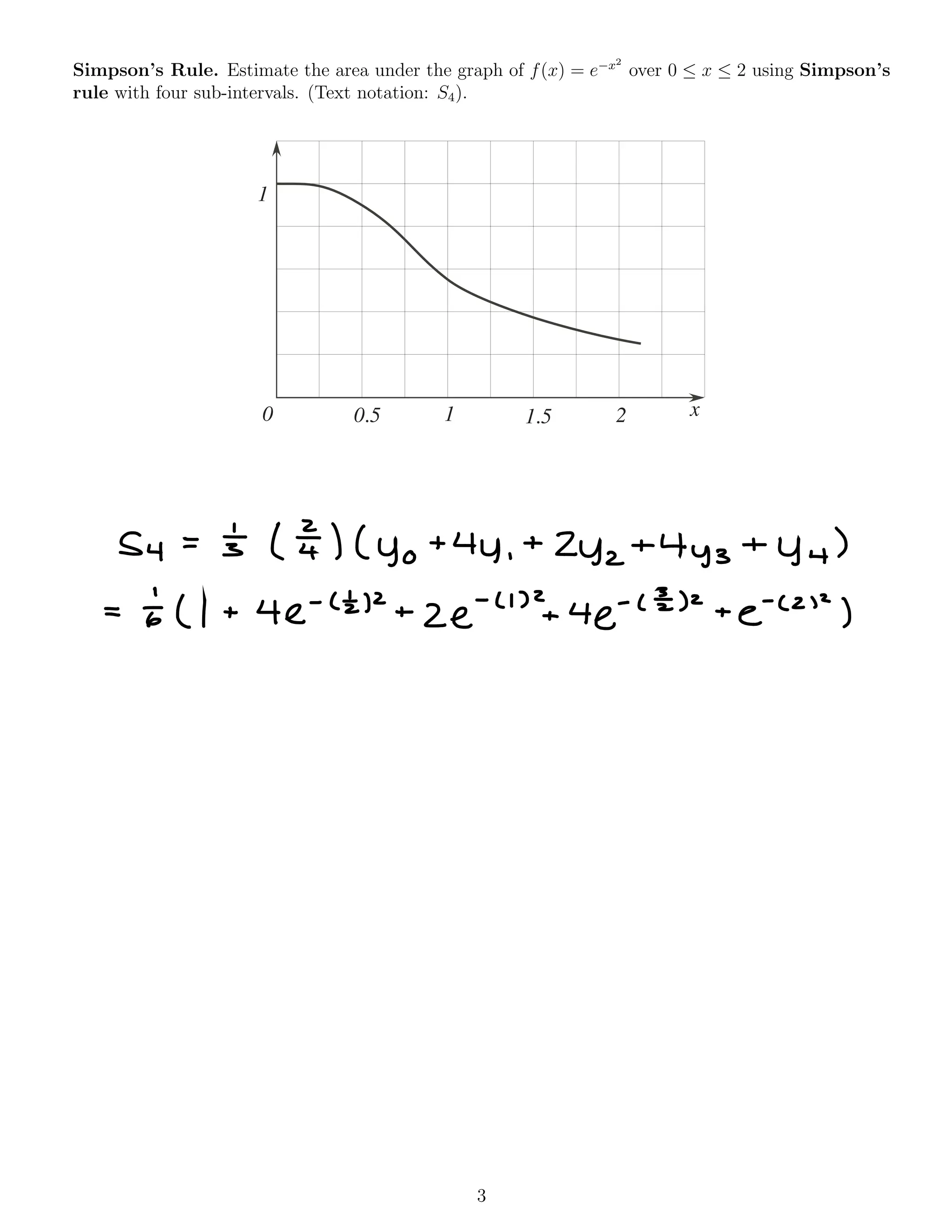
31. Method 3 :
Simpson 's Rule
p ,
f
•
Take 2 adjacent sub -
n intervals [ Xo ,
X ,
]
,
µ•¥Yz✓=
[ x. ,
Xz ]
⇐i
-
-
-
•
Consider the parabola P ,
= .
-
-
-
passing through f ( Xo ) ,
.
-
-
a--
-
b f( × ,
)
, { f( Xz )
to t.dz •
Approximate S Itf< > < s
ox ox
by SIE P
,
dx
=3 ( Dx ) ( yo
+
4y ,
+
yz )
•
Repeat E add up SUM :
SN = 's DX ( yo
.
1
44 , +242+4 Yost
. . .
+
Zyn -
z
+
44N .
,
+
YN )
*
Note that N has to be even

32. Math 10360 – Example Set 05A
7.9 Numerical Integration
Midpoint Rule. Estimate the area under the graph of f(x) = e x2
over 0  x  2 using Midpoint
rule with four sub-intervals. (Text notation: M4).
0
1
0.5 1 1.5 2 x
1
• • • •
o × =
2
I
°
= I
M 4
= £ ( f ( I ) + f ( ÷,
) + f ( I ) +
f ( I ) )
=
I ( e
-
l ÷ )
2
+
e
-
C I )
2
.
e
-
C E ) 2
+
e
-
( ÷ I 2
)

33. Simpson’s Rule. Estimate the area under the graph of f(x) = e x2
over 0  x  2 using Simpson’s
rule with four sub-intervals. (Text notation: S4).
0
1
0.5 1 1.5 2 x
3
54 = 5 ( ¥ ) ( yo +44 ,
+
Zyz+4y3 +44 )
= to ( 1 + 4e
-
( £12 +
ze
.
' ' '
2+4 e-
C E) 2
+
e-
( 2 "
)

34. Integration by Parts
( Indefinite Integrals )
Recall
:S udV= UV
-
SVDU
For definite integration :
Sba udv = Uv 13 -
fbvdu
a
Ex :
Sotxcosxdx
U= × dV= COSXDX
du=dx V =
sihx
xsihx lot -
SE sinxdx
ITS int -
( -
Cos × IE )
0
-
L -
COST + cos 0 )
0 -
( 1 + 1 )
-
2
Trig Integration Techniques
5 sin ( ZX ) ( OS ( 3× ) DX
E 5 sin ( 2×+3×1 + sin ( 2×-3×1 dx
I Ssihcsx ) +
sin C- x ) dx = £ Ssihcsx ) -
sin ( × ) dx
I ( -
stcos ( Sx ) +
COS C- x ) ) + C
5 COS
2
( X ) d X
f 1¥54 dx =
I f 1 +
cos CZX )dx
I ( × +
'
zsinlzx ) ) + C
5 sin 2
( Zx )dX
f lazy =
lz f 1 -
COS ( 4× )

35. 55in 4
( X ) DX
S sin
2
( × ) .
sin
2
( × ) d ×
f ¥4
.
t.co#ax=f*2xftcoI2Idx
LT f I -
ZCOSZX + COS 2C Zx ) DX
LT f I -
ZCOSZX +
1 + COS ( 4 x )
d×
z
f- ( × -
sin Zx +
÷ ( x +
÷ sin ( 4 × ) ) ) +
C
Remark :Ssin
6
( × ) dx = sin
2
( × ) .
sin 4 × ) .
sin
2
( x ) dx
=
S ( In )
3
so this is the strategy that we follow to integrate
Ssihm ( x ) dx ,
SCOSM ( x ) dx ,
When M is even
S sins ( × ) dx
S sin
"
( × ) .
sin ( × ) DX
S ( sin 2
( × ) )
2
.
sin ( × )d×
S ( l -
COS
2
( × ) )2 sink )dX
U =
cos ( × )
du = -
sink
)dx-
du = sin ( x ) DX
-
S ( 1 -
U 2) 2
du
-
S 1 -
242 + U4dU
-
( U
-
Eu 3 + 's Us ) + C
-
( COSX
-
=3 COS 3×+5 COSSX ) +
C
Remark : This is similar for any odd powers of sin E
Cos

36. 50*2 COS (5 × ) COS ( X ) d X
I S 5
' 2
cos Csx + x ) +
COS ( sx -
× ) d ×
£ SE
' 2
COS ( 6 × ) +
COS ( 4 x ) DX
£ ( to sin ( 6 × ) +
Is in ( 4 × ) 1 512
I ( to sin ( 3 Hk't sin ( Zit ) -
0 )
¥0
)

37. Integration Method :
Partial Fractions
Ex : 3×-7 A
+
B ( A E B are
( ×
-
2) ( ×
-
3)
=
×
-
2 ×
-
3 constants )
Multiply both sides by ( X
-
2) ( ×
-
3)
3×-7 = A ( ×
-
3) + B ( × -
2) *
× =3 ¥-9 -
7 =
BC 3 -
2)
B=2
× -
zinxns -
1 =
A (2-3)
A = I
3×-7 I 2
+
( X -
2) ( ×
-
3) ×
-
Z X -
3
Alternatively
:
To find A. B :
Compare coefficients in *
X 3 = A +
B
Constant
-
7 = -3A -
ZB
Solve for A E B
53×2*7+60=5#z +
Fax
=
In 1×-21 + 21h 1×-31 + C
Remark : PFD :
Distinct Linear Factors
p ( × ) , qlx ) polynomials
if degree (D) <
degree ( q )
{ q( × ) = ( ×
-
q , ) .
. .
( ×
-
qn )
Then We Can find A. . . .
,
An
'
=q=×A÷q .
+ .
.
.
team

38. Def :
We Call ±a with deg ( p ) < deg (
q ) a proper
rational function
E × : 2×3 + ×2 -
×
-
1
2×2 -
×
deg ( p ) =3 > deg ( q ) =
2 → not proper
1×+2×2
-
× 2×3
+ ×
2
-
×
-
1
2×3-2×2 -
×
-
1
2×2=-1
2×3 -
×
2 -
×
-
I =
( 2×2 -
× ) ( × + I ) + ( -
l )
2×3 + X
2 -
X
-
1
= × + 1 +
=
2×2 -
X 2×2 -
×
×¥×.
, ,
=
¥ +
B-
¥
2×-1
1 =
A (2×-1) -
BX
× =
0 → I =
A ( 2 ( 0 ) -
l )
A = -
1
× = I → I = I B
B =2
2¥ ×
=
¥ +
¥ ,
f
2×3 + x2 -
× -
I
dx =
S ( x + I +
xt -
¥ ,
) dx
2×2 -
×

39. Ex :
Repeated Linear Factors
× 2 + × + 1
( × + 1) ( × + 4) 2
=
¥1 +
# +
¥+4,2
×
2
+ × + 1 =
A ( X +
4)
2
+ B ( x + 1) ( X +4 ) + ( ( X + 1 )
× =
-
1 →
( -
1)
2
+
C- 1) +1 -
A ( -1 +
4)
2
1 =
9 A
A =
at
X =
-
4 → ( .
4)
2
+
( -
4) + I =
( ( .
4+1 )
13 = -
3C
C =
-
÷
× = 0 → 1 = ÷ ( 4)
2
+ B ( 1) (4) -
¥ ( l )
f ¥+1
B= 4
( X + 1) ( × + 4)
2
A ×
Ex :
Quadratic Factors that are Irreducible
×
-
1
( X 2+1 )×
=
¥ +
BXTCXZ+ I
×
-
1 =
A ( ×2 + 1) + ( BX + C) X
× = 0 → -
1 = ACI )
A - -
1
× = I → 0 =
2A +
( Btc )
×
= -
1 →

40. Recall partial fraction decomposition
Distinct linear :
I A B
X ( × -2 )
X X -2
Repeated linear :
A B
+
C-
( Xtl )3 xtl 1×+112 ( xtl )3
Distinct Irreducible Quadratic :
AX+B CX + D
(112+111×2+2) 112+1 XZ +2

41. Ex
:[ =
f #
DX
X(×2+1 )
x*×2+| )
=
¥ +
BXTCXZ
+ 1
× -
1 =
A 1×2+1 ) + ( BX + C) X = AXZ + A + BXZ + CX
Compare coefficients
XZ :
0 =
A + B →
B =
I
×
:
I =
C
/
Constant : -
l=A
I =
ffxt +
¥+1,
)dx= -
fat +
f # ,
dxtfxazx,
= -
In 1×1 +
I In 1×2+11 + tan
'
( × ) +
C
Improper Integrals
Wenknow Sba is
f
÷
-
= =
= -
= -
,
a b
# → [ a ,
b ]
What about unbounded intervals ?
r
Stao f =
?
Ef
↳
improper
.
=
⇒
,
a R

42. Case 1
Definition
( Improper integrals Over Unbounded intervals )
Stao f ( × ) d × = kinds S I f ( × ) dx
Similarly ,
for
f Is f ( × ) dx = kinda far f ( × ) d ×
Ex : SF 9¥
kinds S ? ¥ =
kinds ( t
'
z ) I F) = trims a Hta -
l ) ) = 1
* We say that SF ¥ is a convergent improper integral
Ex : SF dgx
kimsa ( SR, Ex ) = kinds ( ( In 1×1 ) 17 ) =
kinds ( In IRI -
0 ) = a
* we call this
divergent

43. Case 1 :
( improper integrals Over unbounded intervals )
f {fcx )dX
=p"→% far f ( × ) DX
Question : What about integral of unbounded functions ?
f
¥ .
:R b
Sba f =
Linda +
( Srbf )
Case 2 :
Def .
( Improper integrals for Unbounded
functions )
Ex :
Sj ( xtz ) dx
=kiTo+Sk (9¥ )
=km→o+l÷lk )
=km→o+ ( -
( i -
£ ) )
=
-
1 +
lim
R→o+ £ = as
Divergent

44. Ex :
I =
fj ( ¥3 ) dx
S I ( ¥ . ) dx +
S
o
'
( ¥ ) dx
-
I ,
I 2
I .
=Linfo .
S ? ¥a =
kinso .
( 3 x
' ' 3
I ? )
=
kim→
o
.
( 3 ( R
' ' 3 -
L -
l )
) =3
I z
=
dingo +
S is ¥3 =
kimso + ( 3 ×
" 3
I
'
r
)
=
King o + ( 3 ( l -
R
' ' 3
) ) =3
I =
3 + 3 = 6
Ex :
S I ¥52
S % if'±x .
+
SS ¥7
. .
I .
I z
I ,
=
kinf .
as Spina =
kind.
a ( ±'
arctan ¥ 1 °r )
=
kind .
-
ta ( arctan F ) =
-
±,
. -
E =
Io
Iz =
kima S or ¥1 =
him • ( ÷,
arctan ¥ To )
=
kinds ÷,
larctan E. ) =
't .
E =
too
too +
Io =
LF

45. Ex :
f 5 × e-
×
dx
kinds S ! xe
.
×d×
U= X dV= e
-
×
AX
du = dx V = -
e-
×
x l -
e
'
×
) 1
or
-
for.
e'×d×
' im -
( re
-
R -
I
) -
( e
-
R -
i
)
pmim
k¥+1
+ 1
lim R
R → co Ers
=
kimscsetr = 0
* Choptal Rule
0 + I + I = 2
Functions of 2 or more variables
f( × ,
y ) =
14 -
o÷o ( x
2
+
y2 ) * see week 6 ex
K .
y=x
-
20
HK ) = 14 -
ioo ( XZ + ( ×
-
20 )
2
)
H
'
( × ) =
0
↳ × =
10 →
y
=
-
10
Id .

46. Paramet .
^
Y R={ ( x. g) /
R
01×14 }
< •
>
✓
4 ×
: R={ ( X. g) 1
R 01×14
< • > OEYEG }
V 4
R={ ( X. g) I
•
4
YI
-
X+4 }
y= -
X+4
× c- f-
'
( y )
R •
4

47. Parameterization
^ f
- R={ ( x. y )lyE
-
×+2 }
rzy/Y=
-
×+2
vertical
parameterization
•
if
-
'
(
y )
R={ ( x. y ) 1
XEF
-
'
(
y
) }
R 2
<
✓
•
,
> =
{ ( X. y
) 1×12 -
y }
horizontal parameterization
^
r
R={ ( X. g) IYE
-
×+2 ,
01×12 }
2•
r R={ ( x. g) IOEXEF
-
'
C y ) , 0<-412 }
L -
y
2 -
y
<
✓ ×
•
2
)
,

48. Double Integration
Eaxni
Find
the
volume of the
foyer
%
f( x. y ) = 14 -
o÷o ( ×2+y2 )
T
-
zo
.
y=×
-
20 We FC x. y ) DX by
w V= [ f ( × , y ) OX Dy
Cox ,Dy in R )
X first
VEE
( E ( FC x. y ) .
ox ) )oy-
ZOEY
±0O£×Ef"ly)2o+y
Y ^
Aly ) 2
By taking ox , Oy → 0 ×
V=fIo(580+4 fcx
,y)dx)dy .
£041>
4
Y
zo
=
S .°zo ( 5200+914
-
÷oo(x2+y2 ) )dx)dY
ux*
y
is fixed
= S -
z°o(( 14x -
o÷o ( ¥ +
yzx ) ) 128+4 )
dy
=
f }o ( 14 ( 20 +
y )
-
÷oo( (20*3+42 ( zoty ) ) dy

49. x
y first
Va E ( EFC x. y ) oy ) ox
0<-0×120×-201 OYEO
DX , Dy → 0 Alx )
-
rzv =
5020 ( SI .
zoflxiyldy )dx < %,
Y
>
=
fo20 ( f I. zo
14 -
÷oo ( x2+y2 ) dy ))d×u×
=SY ( my
-
o÷o ( ×2y+ ¥ ) 11 a) dx
Instead of height
:
density
Find the total mass
DM =
( Density ) .
( OA )
f( x. y ) .
ox .
oy eared
EX :
R :
region bounded by y=×2 , y=
-
× ,
×=2
"
I S§ ( 6×2 y+xe4)dA
y first-
2-
×=2
g }§I2×(6×2y+xeY)dy)d×

50. Polar Coordinates
^
% 111 '
.
PCX
,y ) = ( r ,
co )
r = 010<2 't RZO
<
)O
=
>
or
v x
-
it < OEH RIO
x=rcoso
y=rsiho tano=¥
cos @ = I sina.lt
r r
XZ +
y2 - r2
Ex
:(
convert from Cartesian Coordinates to Polar
Coordinates
( 2,53 )
B -
•
( 2,53 ) r2=
22+532--4+3=7r=T7
)0 tan @ =
-5
I
z
2
co =
arctan -32×0.7137 radians
( 3
,
-3 )
( 570.7137 )
} r2= 32+32=9+9--18
)× r=T8 =
352tanx=-32=-1-
3- •
( 3 ,
-3 ) x= -
¥
O= ZIT -
y±= ¥
( 3Vz ,
7*14 )

51. Ex :
Convert polar coordinates to rectangular
coordinates .
( Fz ,
+14 ) × = VZ COS It =
VZ Iz = l
y
=
Vz sin I =
Tz rz =
I
( 1
,
1
)
( 2 ,
7+16 )
cos @ =
cos ( it + × ) = -
COS ×
A = O -
IT =
" '
16 -
IT =
+16
O
-
COS the = -
✓3/z
Sino = sin ( it + a ) = -
sin x
x l
'
-
sin "E =
-
E
X = 2 (
-
B/z ) =
-
B
y
=
2 (
-
'
z ) = - 1
( -
Vs
,
-
1)
Ex : f ( × , y ) =
2×2 +
y2
Write in polar coordinates
f ( × , y ) =
×
2
+
×
2
+
YZ =
×
2
+ r
2
f ( r
,
O )
.
- ( RCOSO )2 + r2
f ( r
,
@ ) =
r
2
COS 20 + r
2
f ( × ,
y
) = 2×2 +
y2 + 2 y±
f ( X.
y
) = ×2 + ×2 +
y2 +
z±y = ×2 + r
2
+
25
=
( RCOSO )
2
+ t 2+2 y±
= TZCOSZ @ + rz + 2 RCOSORsince
f ( r ,
G) = r
2
Cos 20 + r
2
+ ZCOTO

52. Ex :
GRE
set up the total mass comp .
÷ ur
00
,
)Ir
DO
a
a or
or
oA= roo .
or
OM = mass
density
.
DA
= f ( r
,
O ) .
DA
=
f ( r
,
@ ) .
r DO .
Dr
m=§o §"o ( rzcoszotr 2) rdodr

53. Recall :
Diff .
EQS
separable equations
d-Y - p ( × ) .
q ( y )
%÷y ,
dy =
f P ( × ) dx
Ex :
dydx = 3×2
y
flydy =
f 3×2 d ×
Ln I
y
l = ×3 + C
I
y I =
ex
3
+
C
=
e
C .
ex
3
y =
±@
.
ex
3
A → some undetermined constant
y
- A e×3
Ex Set 08A
Application :
Models
involving
Y
'
=
K (
y
-
b )
r a
Constants
d-4 = k ( y
-
b )
at
f ⇒ =
fkdt
Ln 1
y
-
bl = kt + C
I
y
-
b 1 =
ekt
+ C
= ec .
ekt
y
-
b = ± ec ekt
4 = A ekt + b

54. Newton 's Cooling Law :
object
c
surrounding
temp :
? given G constant
=
b
Newton 's Cooling Law :
RateofC@ftemprukLy.b
)
⇒t
Ex 2 ( 08A ) :
Temp of
turkey at time t :
y
( t )
Info :
1
.
Y ( 0 ) =
185
2. room temperature
=
75 = b
3 .
Y ( 30 ) =
150
Problem :
Find y
( 45 )
da-
= K (
y
-
7S )
y
= Aekt +75
185 = A + 75
A =
110
150 =
110 ek
( 30 )
+ 7 s
75 =
110 e
30k
1£ =
@
30k
In (
'
5122 ) -
30k
1<=1*22 ) Since k is negative , y
= Aekttb # b
30
y ( 45 ) = 110 e
k¥022
)
'
45
+ 75

55. Other Models :
¥ = -
3 y
312
tan
2
( t )
y ( 0 ) =
4
Find
y for all time t
For what t do we have y → 0 ?
f #dy = -
3f tan
2
Lt ) dt
.
3¥ ,
y
-
" 2
=
-
3
f 1 + tan
2
L t ) - 1
dt
-
zy
-
' ' 2
= -
3 tan ( t ) + 3t + C
y
-
1/2 = 3/2 tan t -
3/2 t + C
1
4-
' ' 2
=
3/2 tan 0 -
3/2 ( 0 ) + C
'
=
(
'
a =
£
y
- ' 1 2
= 3/2 tant -
3/2 t +
1/2
y
=
( 3/2 (
tant
-
t ) +
'
12 )
-
Z
Y =
( 3/2 ( tant -
t ) +
'
12 )
2
As t → tyz
we have
y
→ 0

56. Recall :
application of ( Separable ) diff .
EQ
'
s
:
-
Newton 's
Cooling Law
-
logistic model
This models the rate of
change of a
quantity y ,
With
growth constant C
Assumption :
y has exponential growth with a maximum
*+
=
Cy ( N -
y )
Solve :
f # y ,
=
of at *
LHS of * :
# ,
=
tyt
+
Fy
I = A ( N -
y ) + B (
y )
y
=
0 → I = A CN )
A =
Nt
y
= N → I =
BCN )
B = th
S
nyttnclny,
dY= Stu ( yt +
n÷y) dy
Alternatively
:
-
1
.
Y + ( N -
y ) ,
yen
.
y )
=
F # =
a # +
ty )
IS ( yttnty ) dy
to ( Lnlyl
-
Ln IN -
y I +
-

57. Nt ( Ln lyl
-
Ln IN -
y
1
) = Ct + B
Lnlyl
-
Ln IN -
y
1 = Nct +
NB
Ln
( ¥1 ) = Not + NB
/
# / =
e.
Nct + NB
=
EN
Ct
@
NB
#
=
( ±
e
NB
) e
Not
-
A
y
=
A e
Not
( N -
y )
y ( l + Nenct ) = A .
enct N
Ae
Nct
N
y
= -
I + Ne Nct
Remark : If
you are
given y
( 0 ) =
-
,
then you can
find A that will give you the particular solutions

58. Ex :
( 08 B -
Zombie Population )
Z ( t ) :
zombie population at time t per thousand
Info :
Z ( t=0 ) = I
N =
40
C = is
logistic model
dzdt =
CZ ( 40
-
z )
z = A e
40 ( ÷o ) +
( 40 -
z ) =
A @
4t
( 40
-
z )
1 = A e4w
)
( 40 -
1) =
39 A
A = sat
Particular solution :
z =
sat e4t ( 40 -
2)
2
( i +
zta e4t ) =
4£ e4t
4013g e
4 t
2 =
1 +
'
13g e4t
* -
z
=
zgle
4T
40 -
z
2-
~ e
-
4t
4-20 ~ e
-
4++1
-
yo
Gets small v. fast
z
→ 1
quickly

59. Recall :
1st Order diff .
equations
dy = f(× ,
y ) K
dx
.
when f( ×
, y ) =
f ( × ) ,
can
#
*
by integration
find y
in terms Of
x.
separable
f( × ) =p ( × ) .
q (
y )
Can solve *
by
Shy ,
dy =
f plx )dx
.
Next :
"
linear
"
first order diff .
EQS
Ex :
×
DI
#
= ezx
d-
dx ( ×
y ) J integrate
×y=Se2×d×
=
'ze2× +
(
y
= xtl 'ze2×t C ) (
general solution )
y ( 1 ) = 0
0
=
÷ ( ÷e2 + C )
0 = I e2 +
C
( = -
tze
2
y=÷(÷e2× -
'ze2 ) ( particular solution )

60. More
generally ,
we can solve linear first order
diff EQ :
-04 + A ( × )
y
= B ( × ) * *
DX
Linear refers to flx , y ) in ¥ =
fcx , y ) being linear in
y
How to solve * *
Idea :
Multiply both sides
by some function I ( × )
I ( × )
#
+ A ( × ) I ( × ) y = B ( x ) I ( X )
⇐I ( × ) .
y ) key Condition
( In previous example ,
I ( X ) = 1)
Find I ( X ) for Ex ( I.
y
) to be equal to LHS
Must have
¥ = A ( × ) I ( × ) + as CI'
yktcxiaat +
FEY
ACXYI ( × )
Question : Can we find I ?
Answer :
Yes ,
+ is a separable diff EQ
f 9¥ =
f A ( x ) dx
Ln I I I = S Adx
I = ± es Adx
Looking for
any
I that satisfies
key
Condition .
SO We will choose to
ignore
I ( × ) = esak 'd×
negative sign 4
integrating constant .
Def : I ( × ) is Called an
integrating factor

61. Ex : Solve the initial value problem
Ay -
tan ( × )
y = I A
*0 ) =3
,
-
±z I × ± tz
-
tan ( × ) =
ALX ) ,
1 =
B ( × )
I ( × ) .
-
e
-
Stan ( × ) dx
S tank ) dx =
SEE dx
u =
cos X
-
f due =
-
↳ I U I + C
= -
Ln I cos × I + C Drop C
-
EE ×<_ E →
Cos × 10
I ( × ) = e
4 ( cos × )
=
cos ×
→ ICOSX 1 =
Cos ×
NOW , Multiply both sides of 4 by COSX
COS ( × ) # -
COS ( × ) tan ( × ) y
=
Cos ( × )
ddx ( cos ( x ) -
y ) = COS 4)
d integrate
y
.
cos ×
= S Cosxdx
=
Sin × + C
y =
tanx +
C-
( general solution )
COSX
3 =
tan LO ) toy ,
=
0 + C =
C
y =
tanx +
costs×
( particular solution )

62. Ex :
×
¥ +
Sy =
¥3
day +
I y
=
e÷→A ( X ) BCX )
I ( × ) =
e
S AK ) d ×
=
e
5 S ¥ =
e
S In ( × ) =
@
in ( x
s
)
I ( × ) =
×
s
MUH both sides by I ( × ) :
dT9 ( y
.
xs ) = ×e×
Integrate to get
:
y
.
×
5
=
f xexdx
4 =
× e
×
d x i dv
du =
DX ex =
V
y
.
×
s
= xe
×
-
ex + C
y = x÷ ( ×e× -
e
×
+
C )

63. Graphical E Numerical Methods
Consider the diff eq .
:
AY = ×2 +
42DX
Point Slope_
( 0,0 ) 0
( 0 ,
0.5 ) ¥
( 0 ,
1 ) 1
( 0 .
5,0 ) ÷,
( 1,0 ) 1
( 05
,
0.5 ) 'z
( I
,
l ) z
( Os ,
i ) E-
( I ,
0.5 ) £
a.
a 9
I 11
It
I
l=-
Can we use this data to approximate
→
-7 what the particular solution looks
05 '
11
I ' '
=
like say assuming YC 01=0.5 ?
<
qFTF DFIELD
0.5 1

64. Euler 's Method :
Linear Approximation
Problem :
⇒ = ×2 +
y2 *
Note :
not linear
If we are given yI)= 0.5 ,
f- ( 0 )
Can we estimate
#
= ?
f- ( 0.1 )
^
o.s.fi#iEIitEeFnrEEyFEiom.8ti5wi+hsiopez
= ( aaf ) ( 0
,
0.5 )
=
, )
0.1
Back to *
y
-
yI)=
(d) ( 0
,
0.5 ) ( x -
0 )
0.5 =
4
y
= 0.5 + ÷ ( × -
o )
is the equation of L
SO the tin .
approx .
Of y ( 0.1 ) :
y ( 0 .
1) = 0.5 + ±,
( 0 .
1) .
-
0.525
Summary :
1. Find the equation of L
2. Find point *
by subbing X =
0.1 in L

65. We can use the estimate
y
( 0 .
1
) =
. 525
and repeat the process to estimate y ( 0 .
2 ) :
y
( 0 .
1 ) +
(date ) ( 0 .
1
,
0 .
525 ) ( x
-
0 .
1 )

66. Euler Method
dY_ = ×
2+42
%0 ) =
0.5
Estimate
y ( 0.3 ) by repeatedly applying linear approximation
Step 1 :
Approximate y ( 0 .
1
) :
^
( 1) /
'
L ,
o .s•
-
¥
Li :
line through ( 0 ,
0.5 )
;
with slope
=
dat ( 0,0 .
5) =
IT
, s EQ Of L ,
:
y = 0.5 +
IT ×
0.1 Yx
'
:
y
( 0.1 ) = 0.5 + LT ( 0 .
1) = 0.525
Step 2 :
Approx .
y( 0.2 ) using approximation y( 0.1 ) in
step I
ask
*l
" 4×2
'
↳
< 2
:
line through
K
, ,k
with slope = aatx ( ¥ )
=
.
=
8¥ ( 0.1 ,
0.525 )
=
=
( 0 .
1) 2.1 ( 0.525 )
2
>
EQ of Lz :
y= 0.525 +
( (0.172+6.525) 2) ( x
-
0.1 )0 !1 & 2
¥
)
:
Approx of y ( 0 .
2) Using ¥ :
0.525 + ( ( 0 .
1)
2 + ( 0.525 ) 2) (0.2-0.1)
= 0.554
Step 3 :
Approx .
y L 0.3 ) Using approximation y ( 0.2 ) in
step 2
n
YLO .
3) a 0.554 + ( CO . 2)
2
+ ( 0.55 4) 2) (0.3-0.2)
(3) =
0.588
(2) * ↳
0554.1111¥¥ * Euler 's method of estimation YCO .
3)
>
wl 3 equal Steps of size 4/1=0.1
to !z o's using YLO ) = 0.5
Note : In each step of size ax we are using
y ( × tax ) ~~y ( × ) + ( dost ) ( × ) .
DX { use the
approximation of y ( × ) in the previous step

67. Mixing Problem :
Ex Set IOC # 2
Tank :
400 ( L ) of Water W/ To € Of chlorine
Italian
400 ( Fo ) =
20g Of chlorine
Incoming
:
4 Lst ) ×
oto LE ) = Too ( ÷ )
- -
concentration
incoming rate of Chlorine
Outgoing :
5 ( ÷ )
×[?](E)_
=
Outgoing rate of chlorine
Concentration
y ( t ) :
quantity of chlorine at time t
Find ylt )

68. Exam 2 Review Packet
2 .
( ×
2
+
1
)
y
'
=
Zxy
-
3 ( × 2+1 )
y ( 1
) = - 1
*
If flx , y ) is a function of ×
,
then solve by integration
*
If f ( ×
, y ) =p ( × ) qly ) :
separable →
separate then
integrate
* If f ( × , y ) is linear in y then use integrating factor
¥
-
×2I+,
y =
-
3
I =
e-SEE , dx U = 112+1
-
S tudu
=
e
-
MU
= a-
'
= ( × 2+15
'
du =
Zx E
duh ( x 2+1 )
'
'
-
¥+1,29 = 3 ( × 2+1 )
-
'
# ×2+1 )
-
'
y ) = 3 ( × 2+1 )
'
'
( ×
2
+ I )
-
'
y
=
-
3 arctanx + C
y
=
( × 2+1 ) ( -3 arctanx + C)
-
1 =
( 2) ( -3 ( +14 ) + C )
3.
Triangular Region
( 1
,
2) ( 1
,
-1 ) ( 2
,
0 )
a
•
Find :
Srs C ( x , y ) da
-
f ? FIYI
4
e× +
6yz dyax
X -
241-2×+4
< i
• s
I I × 1 2
.•
f ? exy +
2y3 /
II
"
ax
f ? e× (-2×+4) + 2 (-2×+4) 3 -
e× ( ×
-
2) -
2 ( X -
2)
3
dx

69. 5.
¥4 =y( ytl ) =
yzty YC
-
2) - 1
Estimate YGI ) in 2 steps
YC
-
1. S ) = 1 + ( 12+1 ) C. S ) =
1+1=2
y(
-
1) = 2+(22+2) C. 5) = 2 +
( 6) C. 5) = 2+3=5
y(
-
1. 5) =
y( -
2) + ( date )(×= -
2 ) .
( .
5 )
y
( -
17 =
YC
-
1. 5) + ( aatx ) ( ×
= -
1.5 ) .
C. S )
9.
flo foF×2 ( xz +
yz )2dyd× y=
Fx 2
Y
2
= 1 -
×
2
ftohfj
(rY2rdrdO=fY
"
florsdrdo1 =
xztyz
Stonier•
I 'o do=p onto do
' -
10A .
Tank :
SO ( L ) ×
to ( the )
:
= 5 ( lb )
incoming :3 ( Ymin ) × To (E)
outgoing
:S( Ymin ) × ? ( ¥ )
date =3 ( ÷ ) -
5
( Shoto )
date
+
stay =3
IOB .

70. Recall :
logistic equation
# =gy
( N -
y ) = ( CN ) y ( l -
F )^
T T
growth maximum intrinsic
rate ( or carrying growth rate
Capacity )
Ex : Set 11A
1. plt ) :
population of fish in thousands
( N = 44,00
N= 105
Extra :
harvesting at rate of 8 thousand per year
a)
E- Yotopll
-
Is ) -
8
b) Sketch the graph of Fai VS .
p and find the point
where # is Max
⇒ =
⇒ PIKE ) -8
•
=( Yotoxnos )( iosp -
pz ) -
o
;
=L ( IOSP -
p2 -
2000 )
1
=
Io ( p
-
zs ) ( p -80 )
(•#ps
Use part b To draw The slope
fields 525 80
Indicate where the slopes are +1-10
÷
oo
-
y y , y y -
If Plt =
01=25 ,
then no
80-41,1*1
,
1,1=1
o Change in Population ,
E same
sG⇐in in p p p p , +
FOR if p(t=O)= 80
40 -
post ggq
↳ Sometimes called equilibrium228=11 1 1 1 1 11 0 Solutions
to to I to t -
t

71. pn If p(t=o ) = 20 →
extinction
Kagy
, y y
1
solution curve for the initial
80 -
balgl*bn1,1,l←ss¥¥a
Value prob . W/ p(t=O ) =
20
SKYEin , p , ↳
Eonguwthocnn
If p(t=0)= 40 → @
40 -
a g g g g q
'
¥aYsF¥EF If p(t=O ) =
100 → 3
25 -
1 ] 1 1 1 | ) 1 ←
threshold
20
#y y y y
( of extinction )
t
f ) .
25 < PCO ) < 80 →
plt ) increases
G tinsoplt )= 80
.
PCO ) < zs →
plt ) decreases to extinction
.
PLO ) > 80 →
p a) decreases
{ times plt ) =
80
( # =
Cp ( N -
p ) )
* )
Note :
this is an example of autonomous diff .
equation
y
'
= FCY ) ( not )
Here for each fixed y slope does not
change
in time

72. Generalized Logistic Equations
Example Set 12A
Recall exponential growth 1 decay model :
by =
Ky ( I )
dt
and logistic model :
⇒+
=
Cy ( N -
y )
=
( CN ) y ( l -
f- ) ( 2)
( and harvesting model :
⇐ =
( CN ) y ( 1- In ) -
harvesting rate )
Introduce Birch Model
dy_ = Al (3)
At N -
y +
Cy
( 1
) { ( 2) are special case of birch model :
*
c =0 →
¥ =
ay
( 1
)
* *
( = 1 →
off =
NE ( y ) ( N -
y ) (2)

73. Ex : h ( t ) :
height of plant at time t
Max height :
5 feet
h Lt ) satisfies :
ath =
go .
#
( * )
5 + 2h
and h LO ) =
2
Problem : How long does it take to reach height = 2 .
S ?
We Will find t in terms of h :
( * ) is separable
f Elk dh =
f For dt
LHS :
¥22 ,
=
f- +
IT
5 +
2h = A ( S -
h ) + Bh
A = 1 B = 3
f th +
IT dh =
foe f At
Ln 1h 1 -
3 Lh 15 -
h 1 =
To t + C
Lh
¥ =
Fo t +
(
Use h ( t =
0 ) = 2
Ln
z÷ = c
t =
to (Ln ( ¥3 ) -
Ln
( I ))
When h =
2.5 ,
+ =
'
EhnEE -
in
÷ )

74. Why introduce Birch model ?
Answer : more
flexibility
Note :
For logistic equation we have :
a =
( CN ) y ( 1
-
Fu )
At
When I is small or y is small then :
dydN
a ( CN )
y
→
y has exponential growth
^
*
EmotionlessTarawa
no
×
SO Max rate of growth happens only when y is small
But for bitch model We have :
•
C > I →
Max rate of growth at
y
< Nz
•
( < I →
Max rate of growth at
y
> E

75. Partial Derivatives
14 .
3
2 .
f ( x , y ) = 3×2 y
b) Derivative of f With respect to X ( With y fixed )
( 3x ) ( ZX ) =
( by ) X
a ) y
=
2
=L ZX
Derivative of f with respect to
y ( with × fixed )
d ) =
3×2
C ) × = 1
=3
Def :
partial Derivative
( 1
) If =
f ×
ox
(2)
¥ =
fy
2nd Partial Derivatives
Def 1 Notation :
fx ×
=
¥ f
×
=
¥
0×2
fyy =
¥ fy =
¥2
fxy = ( f × )
y
=
Fy ( f × )
=
¥
oyax
fyx = ( fy ) × =
¥ ( fy ) =
#
axoy
In this Course , fxy =
fyx

76. Example :
g ( × , y ) =×e×2y
9 ×
=
-3×9 =
ex2y
+×(z×y)e×=
9Y =
§ = ×3 @
xzy
ZX2ye×2y
9××=F× ( 9× )
=
2×ye×2Y +
4xye×2Y +
(2×24) ( Zxy ) e×2Y

77. Estimating Derivatives
^ Slope of L :
f
Ohl f ( at OX ) -
f ( a ) ( , )
Variable
L
ox
'
Yes'in¥ As ox →
other ( 1
)
<
= -
>
1
✓ a atox
d¥ (a)
We Call ( I ) the
"
forward difference estimate
"
of
*
ax
at a .
Similarly , we can define
backward :
n
f ( a ) -
f- ( a -
ox ) f
OX L
f (a)
fca .
ox ) ,
'
41,1¥
<
= -
>
✓ a- ox a
central :
f( a + DX ) -
f ( a -
DX ) ^
2 DX
f ( atlx ) 11 1 11 l I '
fca -
ox , y,
,¥[
<
= = =
< )
✓ a -
ox a atox

78. Similarly ,
We can also define forward ,
backward ,
and central estimates in each variable for
multivariable functions
Estimating partial derivatives
f= f ( × , y )
Forward of :
f ( a + OX ,
b) -
f( a ,
b )
f× at ( a
,
b) Ox
Ex :
Example Set IZB
1. See chart
F= FCT ,
w )
a) Estimate 3¥ at ( 1=-20 ,
W= IS )
Forward
FCZO -
S ,
IS ) -
FC 20,15 )
=
13 -
6
=
75 5 5
Backward
FC2.0.IS ) -
GF
(20-5,15)
=
6
SO =
§Central
1=(20+5,15) -
F ( 20 .
s ,
IS ) 13 -
O 13
= =
-
ZCS ) 10 10

79. Chain Rule for Partial Derivatives
Recall :
one variable :
f=f ( × ) G × =
XCS )
If =
-d× .
If
ds ds DX
Two variables :
f=f( × ,
y ) × =
× ( S ,
t )
y=y
l S ,
t )
df =
Zfx
dx +
#
dy
2 z
Then
⇒ ¥ ⇒ +
⇒ ⇒
¥=¥s÷+¥⇒
f
x
y
s t s t
Same for more variables
22 .
U= Ln ( xztyz )
×= COS Lzt )
y=sih( t )
# = ?
at
du =
¥ dxt
⇒ dy ( I )
# =
Fy¥ +
In
-24ay at
⇐-
dydt At

80. -24 =
# ( 2 )
2 X ×
2
+
y2
*y
=
29×2+
YZ
*
g +
= -
2 sin ( Zt )
-04
= Cost
at
→
⇒ =
(}z÷yz) L -
zsint ) +
( ¥-2 ) cost
Zb .
U =
U ( X
, ,
Xz ,
X 3
)
du =
¥ ax +
Fay ay +
⇒ dz
¥ =
( Ux ) ( xs )
+ ( U
y
) ( y s ) +
( Uz ) ( Zs )
Implicit differentiation :
inter
We say Z is an implicit function of × , y if it satisfies
f ( × , y ,
2) TO
For some function F ( for all values of × , y ,
2 )
→ d F =
0
Fx DX +
Fydy + Fzdz
tiffs Fx ¥ +
Fy a+
Fz -3×2=0wrt x
I I I I
1 0
→
FE -
E÷
€2 = -
#
2 Y Fz

81. Z is an implicit function of × &
y if :
f ( ×
, y ,
z ) = 0
⇒ =¥E ⇒ =¥e
Example
32×3yz
-
y
2 -
3×+2×23+7=0
Zy =
¥2
=
¥29
Fy
'
-
×3z -
Zy
Fz =
×3y + 6×22
Zy =
-1¥
X3y + 6×22
Zy ( I ,
I ,
-
1) = # =
3-
3b .
EYZ +
×+÷z -
5=0
7¥×
=
-
k¥2
Fz =
ye
YZ -
(×¥z)2
Z× =
k¥2
YEYZ -
¥22,2

82. Linear approximation for multivariable functions
Ex Set 13 A
Recall in one variable case
f =f ( x )
n f
EQ
n
of [
:
fcatox ) .
# [ y
-
f (a) = ( ddxt ) ( × =
a ) .
( ×
-
a )
* -
•
•_ -
= -
Slope
( , >
✓
a a + ox Linear approx of flat DX ) :
flat ox ) a f (a) + ( 8¥ ) ( ×= a) ( DX )
fLat_ox)fa= (aa¥ ) ( × =
a ) ( DX )
Of
Multivariable Case :
f = f ( × ,
y )
Lin approx of flatox ,
b +
oy )
f ( a + DX ,
b +
oy ) ~~ f ( a ,
b) +
FI ( a ,
b )
.
DX +
¥y ( a. b)
by
flat Ox , btoy ) -
f ( a ,
b) ~~ FE ( a ,
b) DX +
¥y ( a ,
b) Oy
.f
Example :
Use lin .
approx to estimate the
change in
g ( × , y
) = ×e×2Y when ( × , y ) changes from ( 1,0 ) to
( 0.9 , 0.2 )
( 1
,
0 ) → ( 0.9 ,
0.2 ) DX = 0.9 -
1 = -
0 .
1
Oy =
0.2-0=0.2
Dg a ¥ ( 1,0 ) .
( it ) +
¥ ( 1,0 ) .
( to )
g ×
=
e×2Y +
× ( Zxy ) e×2Y
9 ×
( 1
) =/
gy
= x ( x4e×4 = ×3e×2Y
Dg a
-
to +
to =
to
9 y ( 1
) =/

83. Sensitivity
f = f ( × .
y )
Def : Sensitivity of f wrt x at ( a ,
b) =
3¥ ( a ,
b )
(
sensitivity Coefficient )
.
Sensitivity Of f wrt
y at ( a
,
b) =
¥y ( a ,
b)
Elasticity :
( a ,
b) → ( a +
to a
,
b )
of a ¥x ( a ,
b) ( too a) +
@
no
change in
y direction
Def :
elasticity of f wrt × at ( a , b) =
% Of
change in
f due to it .
change in × = ¥( a ,
b) ( o÷o a)
× 100%
( elasticity coefficient )
f ( a
i
b )
Similarly , elasticity of f
wrty at ( a
,
b)
= ¥y ( a ,
b) ( too b)
f ( a ,
b)
EX 2 :
Cylinder rod W 1
height
=
100 ,
diameter =
5
22 . Volume =
V ( h ,
d ) =
IT (E) 2h =
IT d 2h
( 100 ,
S ) →
100 ± to ,
s ± io
OV a ¥n ( 100 ,
S ) ( ± to ) +
Fa ( 100 ,
s ) ( ± to )
F- =
YI A
2
=
In ( s 2) =
2¥
Tat =
¥ h ( Zd ) =
ZSO it

84. Recall :
Example 2 :
Cylind Rod
Height
:
100
Diameter :S
Volume = ✓ ( h ,
d) = ¥ d 2h
Zb .
Sensitivity of the Volume wrt h at ( 100 ,
S )
=
¥ ( 100 ,
S ) =
YI ( ZS )
sensitivity wrt d
=
¥ ( 100 ,
S ) =
250 IT
ZC .
Elasticity wrth
( 100 ,
5) → ( 100 +
¥100) ,
S )
oh = I
LW a ¥h ( 100 ,
S ) -
I
=
E ( ZS )
Elasticity coefficient = ¥ × 100%
¥ ( ZS )
÷±
(g) ( 100 )
× ' 00% = I %
Elasticity wrtd :
( 100 ,
5) → ( 100 ,
Eis )
od =
zto
LW = Fa ( 100 ,
s ) .
to
=
250 # ( To ) =
I ( 25 )
Elasticity Coeff :
ten
IT (E) ( 100 )
× 100 % = 2%

85. Recall :
Linear Approx
:
f = fcx , y )
( a ,
b ) →
( a +
ox ,
b +
by )
f ( a + DX ,
b + D y ) a f- ( a ,
b) + 3¥ ( a
,
b ) .
Ox +
Fy ( a ,
b) Oy
of a FE ( a ,
b ) .
DX +
¥y ( a ,
b) Oy
More examples :
3 .
200 ft
100ft
I 3 inch
;
Problem :
Use tin approx to
inch find the area Of the frame
A =
A ( × , y ) =
xy
I A =
A ( 200 +
£ ,
100++2 ) -
A ( 200 ,
100 )
~~ ¥ ( 200 ,
100 ) ( I ) +
¥ ( 200 ,
100 ) ( I )
=
100 ( E) +200 ( I ) =
ISO

86. Example set 13
1
.
Approx f ( -0.8 ,
2. 2)
Using
the value of fat
( -
0 . s ,
2 )
( -0.5 ,
2) → ( -0 .
8 ,
2 . 2)
Ox = -
0 .
8+0.5 = -0.3
Oy = 2 .
2
-
2 =
.
2
f ( -
0 .
8 ,
2. 2) a f- C- 0 .
s
,
2) +
¥ ( -0.5 ,
2) ( -0 .
3) +
¥y TO .S
,
2) C. 2)
* Use chart
-
5
3×1 to .s ,
2) = ?
Backward :
f ( -0 .
5 ,
2) -
f ( -1 , 2) =
S -
4 .
5
= ,
Approx . S .
5
ofy
( -
0.5
,
2) = ?
Forward :
f ( -0.5 ,
2.
5.)gift
0.5 ,
2)
=
6 .
If
5
= z . z
Approx
Sub Back
Lagrange Multipliers
Problem :
Given f ( × , y ) ,
find the points Lx , y )
Satisfying g ( × , y ) = 0 ,
Where the function FC × , y )
reaches its Max or min
Def :
Level Sets :
Points ( × , y ) that satisfy f ( × , y ) =
C for Some
constant C T
intersection of f w1 horiz . plane 2 -
C
Key Idea : the points we are looking for happen where :
level
sets and g ( x ,
y ) =O share the same tangent direction after
projectiononto xy
-
plane

87. 1.
Tangent to f=C at ( x , y ) =
tangent to
g
2.
g ( × , y
) = 0
Q :
HOW to find ddxt for FCX , y ) =C ?
Implicit diff :
dy =
-
fx
dx fy
similarly ,
dy =
-
9 ×
dx gy
1.
¥ =
sgxyn
at ( x , y )
→ ( f × , fy ) = X .
( g × , gy )
→
so we have to solve :
If
= ×
#
at ( × , y )
ax ox
If = ×
-09
at ( X , y )
oy Zy
g( x. y ) = 0
Example Set 13C
Ex :
la .
height of roof : h ( × , y ) =
2×+4 y + 20
Spider 's Path :
×2 +
y2 =
4
g
=
×2ty2
-
4
Solve :
*
y¥o
hx -
Xgx 2 = X ( Zx )
hy =
Xgy
I 4 =
× ( zy )
→
÷ =
I =
y±
g
= 0
y=z×
XZ + ( Zx ) 2
= 4 =
5×2
×=±
; Its ,
Es )
y = ±
IF f Ers
,
-
Is )

88. h ( r÷ ,
Is
)=
4 is +20
h
( -
Is ,
-
Is ) =
-
4 is + 20
when
y
= 0 → × = ± z
h ( ± 2 ,
0 ) =
20 ± 4
SO Max
=
4 is +20 at ( Is ,
Fst )
min =
20 -
4 is at t÷ ,
-
Fs )
lb .
If the path is a semicircle maxlmih could
happen at endpoints ,
when path is not closed
h ( 2 ,
0 ) =
4 + 20 =
24
h C- 2 ,
0 ) = -
4 + 20 = 16
( ⇒ ,
-
Ffs ) is not part of the new path
so min =
16
2 .
P =
60 k
' 14
[
3/4
30 ,
000=15 K + 3L ←
g
Solve Pk =
X 9 k
PL =
XGL
g
= 0
P k
=
IS K
-
3/4
L
314
PL =
45 k 114
[
114
/ S K
-
314
L
3/4
= × .
IS
45 k
' ' 4
[
' 14
=
X .
3
's 15
'
L = S
L = 15 k
IS K + 3 ( 15 ) K = 30000
k = SOO
L = 1
S ( SOO )

89. Sequence and Series
Example Set 14A :
.
sequence
:
an ordered
listing of numbers n
an
.
Sequence Of odd numbers : 1
,
3 ,
5 ,
7 ,
9 ,
...
-
Or a =
2h - 1
-
•
n .
-
•
a ,
=L -
-
•
az =3 -
23=5 =
•
{ an }F= ,
-
•
(
✓
I I I I I I )
'
Sequence Of powers of I
bnr
lim
n
n → a
an = as
bn = ( it
"
I -
•
b. =
I lim
n→abn=O
bz= KY l -
•
4
b3= ( EP l - •
8
{ bn }F=l c i 1 1 >
✓ n
Find limits :
lim
1 -
e2n + 4e6n
h→•
( 3 +
Sen +
econ)=4= him .
-4%1=4
lim
n→•
COS ( ht ) = DNE
h=1 :
COS ( A) = -
1
h=2 :
Cos ( ZT ) = 1
n =3 :
COS ( 3T ) = -
1
SO COS ( hit )
{
-
1
,
n Odd
=
( y )n
1
,
n even
Limit Laws :
Assume
thinks ( an ) and hinto (
bn
) both exist ( *
a. not
divergent )
1. hinfo ( an ±
bn )=hi→mo( an )±n"Too ( bn )
2. Lisa ( an bn )= ( n'irsoankninsabn )
3. himo (E) tree
lim
n→abn
4. dish ( C .
an )= c. high an
T
Constant

90. Squeeze Theorem
{ an } ,
{ bn } .
{ Cn } 3 sequences
an I bn E Cn
for every n ( or for some n 2 M ,
M c IN
If high an = hints Cn =L
Then Links bn =L
lim
n → a ( ein sin ( h ) ) =
0
-
11 sin ( h ) El
-
e
-
nee
'
hsin ( n ) E ein
t t
o 0
By squeeze theorem → him a ( Ens in ( n ) ) =
0
Def :
geometric sequence
{ an }F= , if for every n we have
an + I
an
= r ← Common ratio
for some fixed r
÷ ,
kt ,
hp
i
2 2
so a ,
=
C
az
=
Cr
23 = Cr
2
24
=
Cr
3
an =
crn
-
'
Alternatively ,
we can start at 0
ao =
C
a ,
=
Cr
dz =
C p
2
an
=
Crn

91. za ) { tz ,
÷ ,
÷ .
÷ , ...
}
an
= #
not
geometriclim
n → as an =/
zb ) { -
s±
,
E ,
-
¥ ,
¥ , ...
}
÷ . .
÷= .
÷
-
E .
¥= .
÷
geometric
an =
f÷ ) f ± )
n
lim
n → a an = 0
ZC ) Cn + ,
=
( n + I ) Cn for n >_ I and C ,
= I
C ,
= 1
Cz =
( I + 1 ) ( I ) =
2
Cz =
( 2+1 ) ( 2) =
6
lim
n → as
Cn = Cs

92. Def :
Series is the sum of all terms of a sequence
{ an }F=i
=
a ,
+ a z
+
23 + . . .
:[ an
:Ummation notation :
53 =
§ ,
a
k
= a
,
+
az + a
3
Sn =
§,
a
k
= a
,
+ . . .
+
an ( Nth partial sum )
so
§,
an =
n'info ( Sn )
More on
geometric sequences and series
Example Set 14 B
1. ball projected 10ft E bounces at 801 .
of previous height
10 ,
1010.8 ) ,
10 ( 0 . 8)
2
,
10 ( 0 .
8)
n -
'
hn =
10 ( 0.8 )
n -
'
C = 10 ,
r = 0.8
So = 101¥ ) =
⇒ SO
2 ( SO ) =
100 ( bk
goes up E down )
Def :
Geometric Series
=
sum of all terms in the
geometric sequence { Crn }F=o
=
C + Cr + C r
2
+ . . .
+
c to
a C rn
h = 0
or { crn
'
'
}F= ,
a C rn
-
i
n = 1

93. Claim :
an =
c .
rn
-
'
{ an } F- I
S n
=
§,
C rn
-
'
=
C + Cr + C r
2
+ . . .
+
cr
N -
I
=
cliIn 1
Proof
t.SN =
Cr + Cr
2
+ Cr
3 + . . . +
Cr
N - 1
+
Cr
N
Sn
-
r SN =
C -
Cr
N
=
c ( 1 -
rn )
Sn ( 1 -
r ) =
C ( 1 -
rn )
Sn =
c ( ¥ )
E. c. rn
'
=
n'i→ma ( sn I =
n'into Klein ) ) =
{ufnraeiiined!ItYrhi
3 a ) F -
as +
ET -
if + . . .
C =
I ,
r =
-
's
⇐ It 's In
"
=
n'info sn =
if =
F
3 "
I ¥ =
EE
,
l÷ in =
E o
last -
( I +
÷ +
t⇐DN E Sz
bk 4/3 > 1
↳
E.3
¥ dogspiomit+
have
5 .
Rewrite as fractions
5 a ) 0.9 =
0 .
9999 . . .
=
to +
÷o +
÷oo+ . . . = EE
,
( Fo ) l ÷o)
n '
'
= Fo ( i÷÷ ) =
To .
'
÷ = 1

94. Sb ) 3. OII
=3 + ( 12×10
-
3) +
( 12×10
's
) +
( 12×10-7 ) + . . .
=
3 +
n§
,
( 12×10
-
3) ( 10
-
2)
n -
I
=3 + ( 12×10
-
s
) ( ¥2 )
=3 +
( 12×10
's
) (
'
fat )
=3 + hat × to =3 +
Is =
YET

95. Recall :
1 .
rmi '
1 + r + r
2 + . . .
+
r
m
= Fr
Notation :
SN =
sum of first n terms
Ex : { an }F=i , an =
c. rn
'
'
SN =
C + Cr + . . . +
cr
n -
'
=
c ( Fn )
T 4
a ,
an
{ an } F. o ,
an = c. rn
Sn =
C -
cr + . . .
+ cr
N -
'
=
( ( Ff )
T In
do 2 N -
1
Example Set 14C :
1.
Day
0 :
30
←
Xo
1 : To ( 30 ) + 30 ← X ,
2 : I (To(301+30)+30←
xz
↳ =
( to ) 2130) + to 130 ) +30
Xn = 30 + ( To ) ( 30 ) +
(E) 430 ) + . . .
+
( To )
"
( 30 )
Day 2 before the next dose is
given
:
Xz
-
30
Day n before the next dose is given
:
xn
-
30
Xn -
30 = To ( 30 ) ( 1 +
to +
( E)
2
+ . . .
+
(To )
n '
'
)
=
Fo ( 30 ) ( ¥91
"
) = 4s
( l -
( to )
"
)
Long term measurement before the next dose is given
:
n
"→ma ( 45 ( 1 -
( to )
"
) ) = 4s

96. Za ) Xo =
100
X ,
=
100 + to ( 100 ) -
Fo ( 100 ) =
100 ( To )
Xn+ ,
=
Xn
-
to ( × n
)
=
Fo Xn
Xo :
100
× ,
: Fo ( 100 )
xz
:
l Fo) 4100 )
xn
:
( E)
"
( 100 )
so { xn }F=o is a geometric series
Zb ) Xn + ,
= ( Fo ) × n
+ I
X o
:
100
× ,
:( to ) ( 100 ) + Fo
xz
:
I ÷o)l÷o l 100 ) +
E) +
Fo =
( ÷ ) 21100k (E) (E) +
Fo
xn
=
( To )
"
( 100 ) +
[ Fo +
Fo ( E) +
to ( E) 2+ . . .
+
( E) (E)
m '
]
=
( to Yu oo ) +
Fo .
HEE (E)
"
( 1001+811 -
l÷o )
"
)
As n → A
,
xn
→ 8

97. A note on elasticity
:
Wrt × :
( a ,
b) →
( a + iota ,
b)
If = f× ( a ,
b ) .
( ioo a )
Elasticity wrtx at ( a ,
b) = fx ( a , b) iota × 100% =
¥ × 100 %
f ( a ,
b)
E if given
table
Ex : f ( × , y ) = e×Y
f ×
=
ye
×Y
elasticity wrtx at ( 2.1 ) :
fx ( 2 , 1) '
too (2) =
EZ -
2
=
z
f ( 2 ,
1 ) e
2

98. Computing Infinite Series
( Set 15 b)
Recall geometric series
⇐ c.
renting .
c
thy
SN
If I r 1<1 → ( ( I )
In addition to this there is another set of standard examples where we can
Compute the a -
series :
telescopic series
Ex :
S =
EE
,
t ,
=
÷ +
at +
÷ + . . .
k¥1 FIt -
¥ =
lek
K ( kt I )
partial fraction decomposition
S =
EE
,
÷ -
In
sn=E. ,
÷ -
±=k -
tzttl 's -
tttl 's -
It + it
# -
tnttfn -
n÷,
)
= 1 -
nt ,
s =
winds Sn =
dingo ( l -
n÷, ) =L
What about S = EE ¥+2 ?
¥+2 , =÷Ii÷t= It ÷ -
±zt .
EE,
{ He -
¥1 +1¥ -
¥1
→
sn =
's §,
it -
he )=E{ ( I -
n÷,
) +
ltzntz ) }
S =
tnimsasn =
zt ( i + tz )

99. A
Ex
:s=E
1<=3

100. Convergence of Infinite Series
Ratio Test
s=E an
Define e - dba / ¥1
If e < 1 → S
converges
If e > 1 → S has no limits
If e = I → inconclusive
Ex :
Za )
s = £ I -
7)
"
n = 1
n÷
let k¥I¥i
him n
n → ants = I
C =Linfo I -7
¥, ,s
/ = 7 > I → no limits
A
n
Zb ) s = [
2h=
O
n !
l¥th¥l
hints ¥n .
=
ntinto ¥ =
o
e =
nlinfo ( 2 -
ant ) =
0
→
by ratio test ,
S
converges
co
ZC )
s =
E
nh= |
N +2
# .
#
n +3 n
C = 1 →
inconclusive

101. But in
general ,
if an 1- 0 ,
then E an has no limits
Power Series :
Def :
We Call
co
S ( x ) = E an ( x -
C )
"
T n = 0 T
function Constant
Of X
=
a o
+ a ,
( ×
-
C ) +
a z
( ×
-
C)
2
+ . . .
A power series centered atc
we will address 2 questions
:
I .
For what values of × does s ( × )
converge ?
2. smooth functions as power series
Convergence
Def :
Given power series S ( × )
we call a non negative number R C
including + A ) the radius of
convergence if S ( x )
Converges for all ×
satisfying
1
× -
C I < R
r
c-
I I 1
ofq
convergent
and has no limits for all ×
satisfying
1
x
-
C 1 > R
To find R :
Use ratio test
co
3a )
s ( × ) = E
#
"
n = 1 n
3
k¥25" Ertl # pix
.
a 1
Ask → co
| ¥3,3 ( × -
2)
| → 1×-21
By ratio test S ( × )
converges if 1×-21<1 { has no limits if 1×-21>1
R = 1

102. Radius of
Convergence
Ex :
3b ) s ( × ) = £ ×2k
K 2kt I
let 't=k÷IIax÷tkE÷sl
As K → a
1×21 =
1×12
SK )
Converges if
1×12<1 ←>
1×1<1
R = 1

103. Taylor Series for Smooth Functions
Example Set 16A
Smooth Function = have differentiable derivatives of all orders
Recall
÷× = I + × + ×
2
+ ×
3
+ . . .
a < 1
SO 1 is the radius of
convergence of the power series on the RHS
and I + x + x2 + . . .
is a power series representation of ÷x over
-
17×71
centered at 0
Similar Examples
Find a power series representation for
f ( × ) =
z÷× centered at 0
z?×=÷ It )
=
3z ( I +
÷ x +
( Ix )
2
+
. . .
)
I × 1
< 2 =
I +
÷ x +
3z×2 + . . .
T
R
NOW centered at C- I )
T?×=F×3t=3÷× , ,
=3
,÷¥
,
F
I +
¥1 +
( ¥
)2+
. . .
÷ 1<1 ←> 1×+11 <3
p
R

104. Q :
Can We find such power series representation for other smooth
functions ?
Yes .
Suppose we can
Centered at 0 :
f ( × ) =
a o
+
a ,
× + a 2×2 + . . .
→
a o
=
f ( 0 )
f
'
( x ) = a ,
+
Zaz × + 3 a 3×2 + . . .
→
f
'
( 0 ) =
a ,
f
"
( x ) =
Zaz +
6 a
3
× + . . .
f
"
( 0 ) =
Zaz
→
a z
-
zt f
( 2)
( 0 )
a 3
=
to
f
' 3 '
( 0 )
an
=
n÷ f
' n'
( 0 )
→ f ( x )
=§o ¥40
'
xn
Centered at C
f ( x ) =
do
+
a ,
( × -
c ) +
a 2
( ×
.
C )
2
+ . . .
Evaluate f at C
f ( ( ) =
a o
f
'
( ( ) =
a ,
an = n÷ f
' n'
( ( )
→ f ( × )
=n§o nah
)
( × -
c)
n
Def :
Taylor Series
We call TCX ) =
⇐ ¥54 ( ×
-
c)
n
the Taylor Series of f at C ( or centered at C )

105. Def :
Taylor Polynomial
Given TH )
=§o fly '
( ×
-
c)
n
We Call the deg -
Nth part ( sum of polynomials in TCX ) of degree
IN ) of TCX ) the Ntt
'
Taylor Polynomial
Notation :
Tn ( × )
EX :
To ( × ) =
do
=
f ( C )
Tz ( × ) =
f ( c ) + f
'
( c ) ( × -
c ) +
¥9
'
( ×
.
c)
2
→ TH ) = discs ( Tn ( × ) )
Def :
When C= 0 ,
we call the Taylor Series TCX ) the Maclaurin
Series
* In this Class ,
we Will assume that Over domain off 4 wlin the
radius Of Cohv .
Of TCX ) we have : f ( X ) =
TCX )
The
geometric series are all examples of Taylor Series :
# = 1 + × + ×
2
+ . . i
-
Tko ) Ito ) .
x
f
1×1 < 1
# =p÷ +
÷ × +
38×2 + . . .
⇒2
f ( 0 ) f
'
( 0 ) .
×
⇐×
,
Imation,
+
# + . . .

106. Za ) Find TCX ) for e
×
at 0
f- ( × ) =
e
×
f ( 0 ) = 1
,
f
'
( 0 ) = 1
,
f
' '
( 0 ) =
I
,
f
( n '
( 0 ) =
/
→ text
EIo±LY0xn=Eo #
= 1 + n +
¥ +
¥ + . . .
The interval of
Convergence
×
nt '
.
n ! ×
( nil ) ! Xn ( nil )
IS 0 < 1
4
for all X
ratio test → the radius of corn .
= A
→
interval =
R

107. Recall :
Find TCX ) for e× at 0 :
Tineo ¥9 ×n=nE=o ¥
Zb ) Estimate e° '
2
using 4th
Taylor Poly Ii ( x )
Ta ( × ) =n&o¥n =
I + × + ¥ +
¥ "
'¥
f ( × ) =T( X ) wl in radius Of corn .
f ( × ) ~~ TN ( x )
f ( 0.2 ) ~~ Ty ( 0.2 )
= 1 +
To +
tz (÷o )
2
+
at ( to )3+ at ( to )
"
= 1.2214
Remark :
fC0)+f'(0)×_
=
linear approximation
T ,
at to
T ,
( ÷o ) =
f ( 0 ) + f
'
( 0 ) ( E) =
lin approx .
of f ( To ) at 0
÷c) Write down the error of this estimate .
Error = ( f ( × ) -
Ty ( × ) ) ( 0.2 )
* )
a Of
n=S n !
Example Set 16 B
I .
f ( × ) =
Lh ( × + 2)
Find Is ( x ) at -1
I ( x ) =n&o ¥7 '
( x +
1)
n
f ( -
1) =
Ln ( l ) =
Of'tn= #
kiri }IYYIYY¥I¥hEt¥tI,Yt
' "
f
"
( -
1) =
¥2,2 ( -
1 ) = -
1
f ' 3)
tl ) =
1+-2,3 (-1 ) =
2

108. Use previous answer to estimate In ( 0.8 )
Lh ( X + 2) a Ts ( × )
Ln ( 0 .
8) =
Lh ( -
1
.
2+2 ) ~~
Tz ( -
1. 2)
-
×
=
( -
1. 2 + 1 ) -
zt ( -0 .
2)
2
+ 's ( -0 .
2)
3
2 .
Use the Taylor Series for i÷x at 0 to find the one for u¥z)z
Observation :
¥a= Fox ( ¥ )
1- =
1-
I + ×2 1- ( -
×2 )
co co
=
E ( -
× 2)
n
= E ( -
1) n×2n
T n = 0 n=o
1×21<1
¥XZ
=
¥ ( §o th
"
x2n
) =§?o # ( ( -
hnxzn )
=n⇐,
fax ( ( -
i ) nxzn )
co
= [ ( -
1)
n
( 2h ) ×2n
-
l
n=O
a
Change to 1
0 ! = 1
4 b) Find B at I for y ( t ) ; the solution of y
'
=
y
2
+
ty , y ( 1) = -
I
I
ltl=&o Yad ( t -
1)
n
Y ( 1) = -
1
Y
'
( l ) = ( -
1)
2
+
( 1) ( -1 ) = 0
Y
' '
( l ) = ?
y
' '
=
Zy y
'
+
y
+
ty
'
→
Y
' '
( 1 ) = 2( -
1) ( 0 ) + ( -
1
) + 0 = - 1

109. Y
' ' '
= 2 ( y
'
FtZy y
' '
+
y
'
+
y
'
+ t
y
' '
Y
' ' '
( 1
) = 2 ( 0 )
2
+
2C -
1) ( -
1 ) +0 +
0 + ( 1 ) ( -
1
) = 1
Y ( t ) a Tz ( t ) = -
1
-
£ ( t -
1)
2
+ z÷ ( t -
1 )
3
3 a 1 Use Taylor Series itxz to find the one for tah
'
'
( x ) over
-
1 < × < l
fax = tah
-
'
( x 7 + C
# =
¥2 ,
=
§o tx 2)
n
=n⇐o t 1)
n
xzn
tan
- '
( × ) +
C
=
f§=o thn
x2ndX=nEo( f thnxzndx )
=
§o C- 1
)
n
In ×
2h +1
To find C
,
evaluate both sides at × =
0 :
0 + C = 0 → C =
0