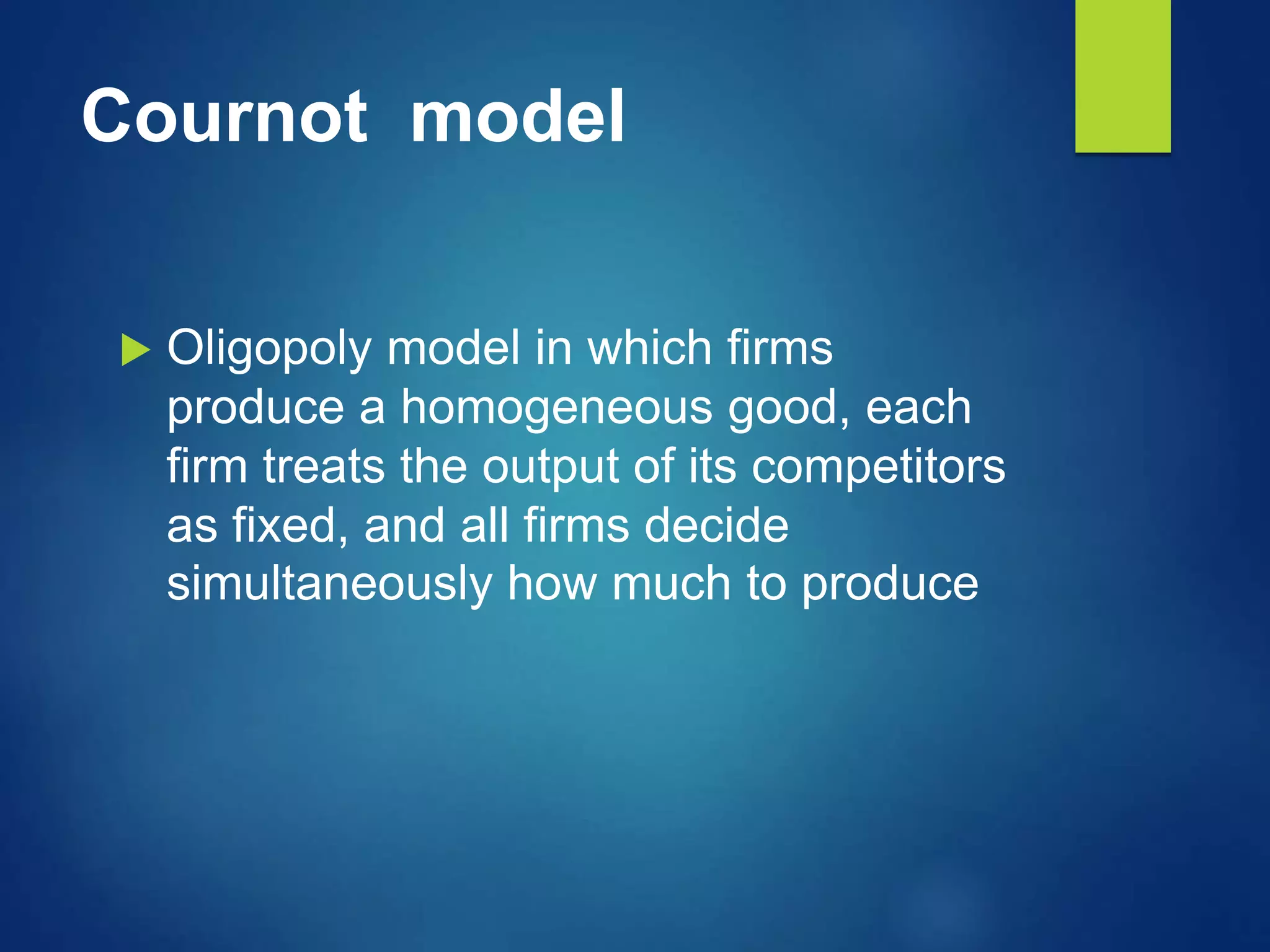
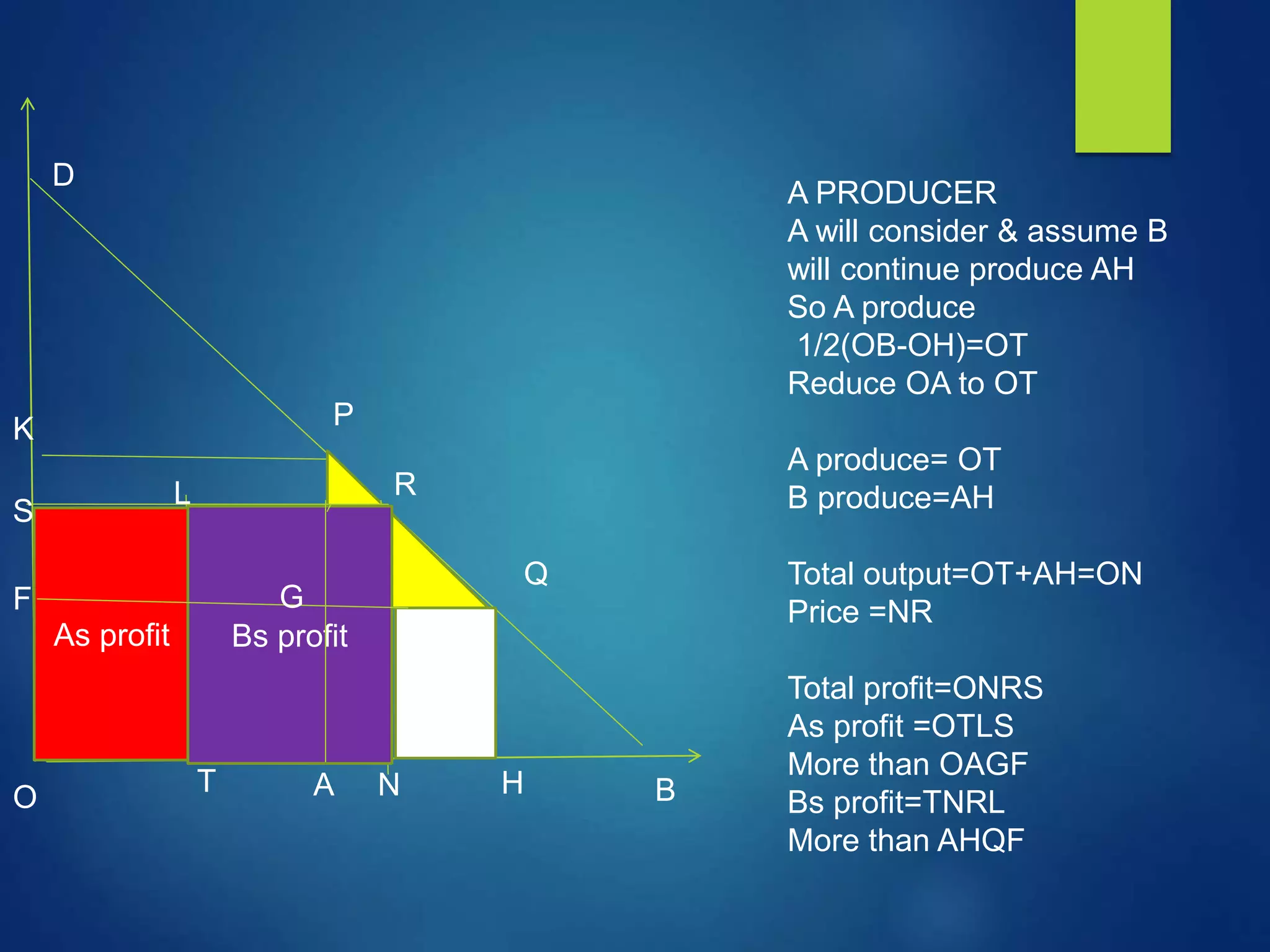
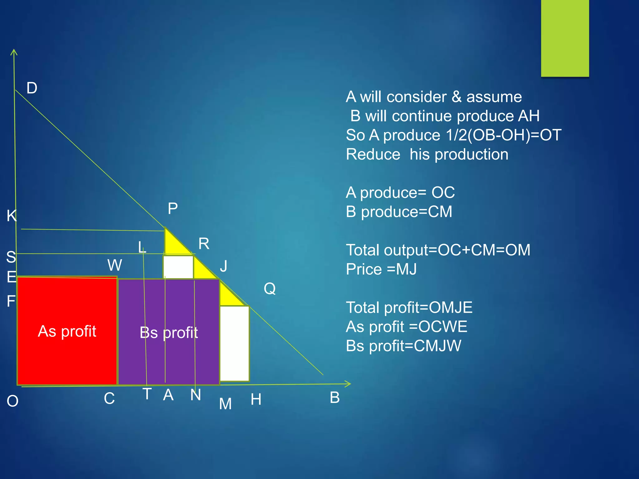
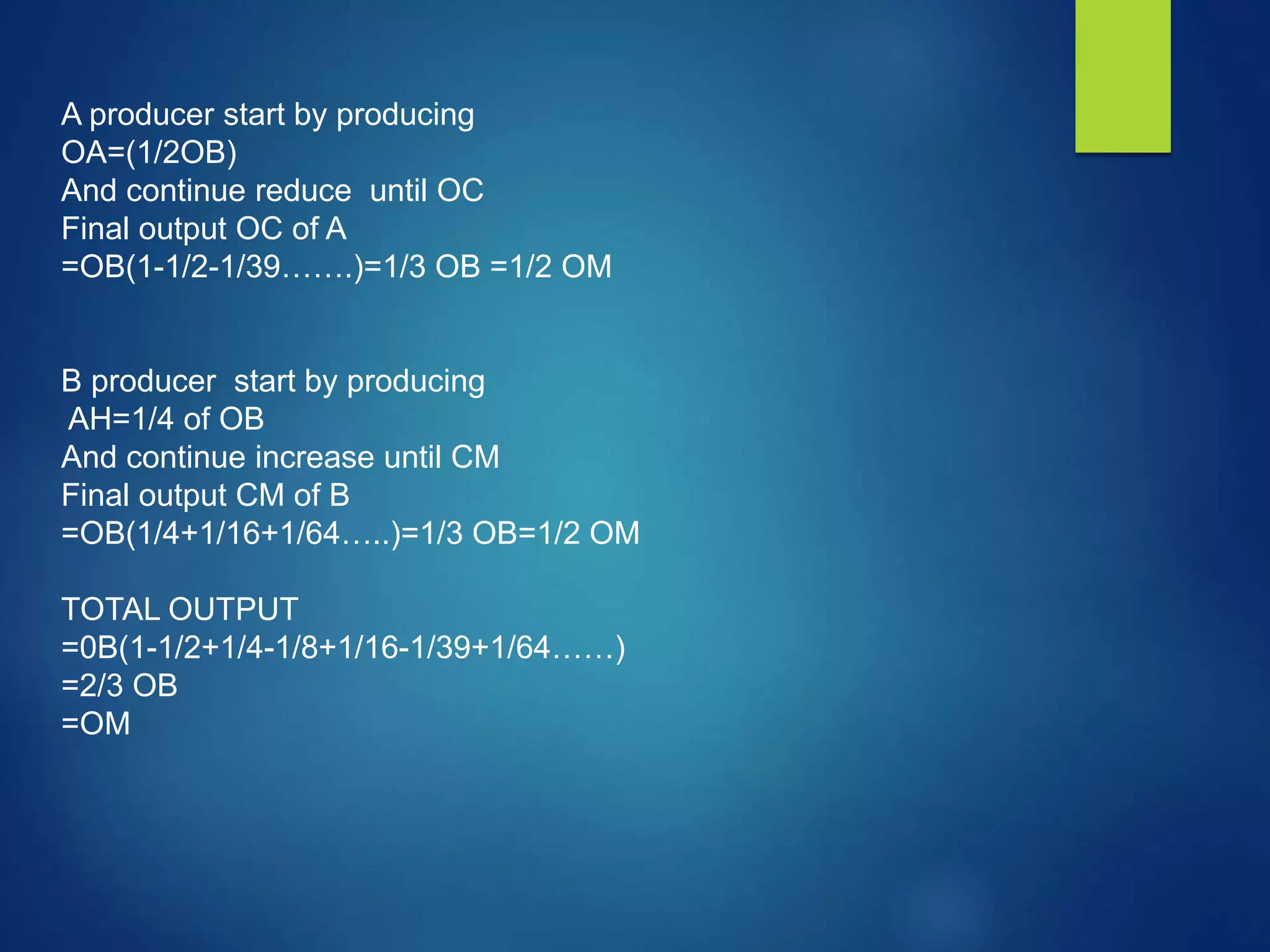
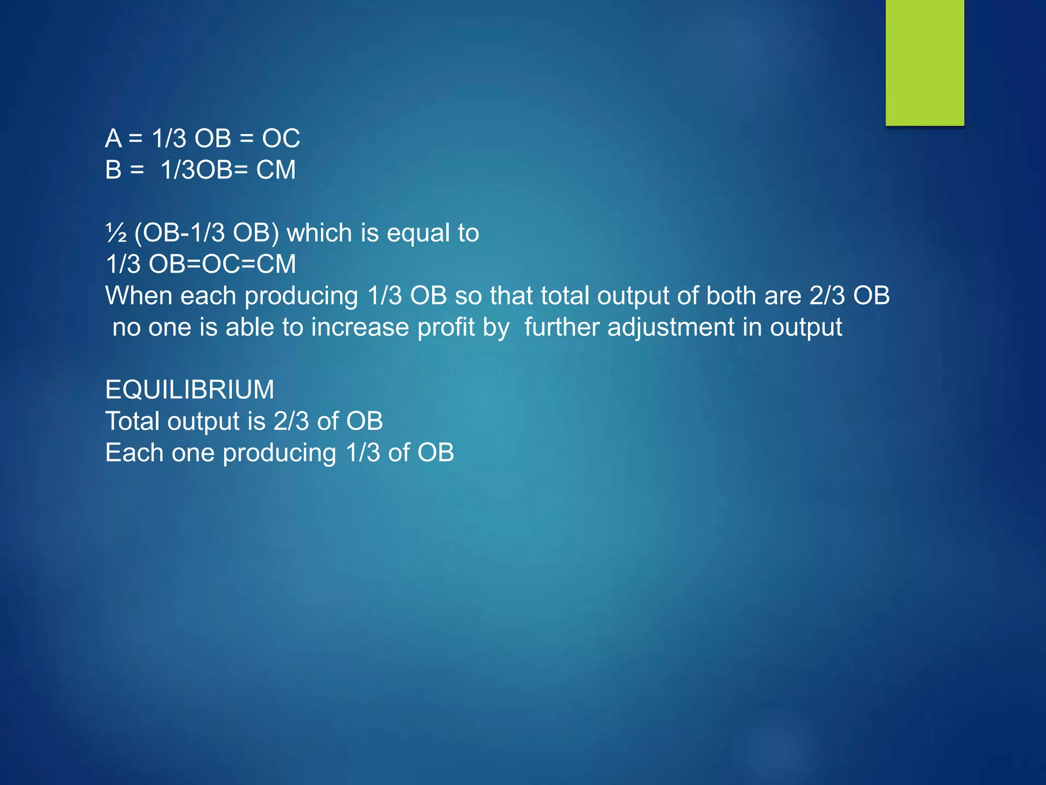
This document provides an overview of the Cournot model for duopoly markets. The key points are: 1) The Cournot model assumes two firms produce a homogeneous good, each treats the other's output as fixed, and they decide quantity simultaneously. 2) Through a process of adjustment and readjustment, each firm will gradually reduce or increase production until equilibrium is reached where both firms produce 1/3 of the total market output and maximize their profits. 3) The equilibrium point occurs when no firm can increase profits by altering their quantity unilaterally, and total output is 2/3 of the maximum market quantity.

1. COURNOT MODEL FOR
DUOPOLY MARKET

2. Presented by,
Yagnesh Sondarva
04-2664-2015
MSc. Agri.Extension
BACA, Anand

3. Market Structure
1) Number of firms in market
2) Product Differentiation
Markets are often described by the degree of concentration
Monopoly is one extreme with the highest concentration - one seller
Perfect competition is the other extreme with innumerable sellers
Oligopoly involves few sellers engaging in strategic competition

4. Number of Sellers
Degree of
Product
Differentiation
Many Few One
Dominant
One
Firms produce
identical
products
Perfect
Competition
Oligopoly with
homogeneous
products
Dominant
firm
Monopoly
Firms produce
differentiated
products
Monopolistic
Competition
Oligopoly with
differentiated
products
------------ ------------

5. PERFECT

6. Perfect Competition
1) Many Firms
2) Homogeneous Products
examples: farm commodities like wheat, Pulses

7. Monopolistic Competition
1) Many Firms
2) Differentiated Products
Examples: retail trade

8. Monopoly
1) One Firm
2) One Product
Example : railway , post , electricity, Insurance
(government monopoly)

9. Oligopoly
A) Homogeneous Products Oligopoly
1) Few Firms
2) Homogeneous Products
Examples: steel ,chemical.
B) Differentiated Products Oligopoly
1) Few Firms
2) Differentiated Products
Examples: automobile , computer

10. Oligopoly
 Market has a small number of sellers
 Pricing and output decisions by each firm affects the
price and output in the industry
 Oligopoly models (Cournot, Bertrand) focus on how
firms react to each other’s moves

11. Oligopoly – Characteristics
 Product differentiation may or may not exist
 Barriers to entry
 Small number of firms
 Scale economies
 Patents
 Technology
 Name recognition
 Strategic action

12. Oligopoly
 Examples
 Automobiles
 Steel
 Aluminum
 Petrochemicals
 Electrical equipment

13. Management Challenges
 Strategic actions to deter entry
 Threaten to decrease price against new competitors by
keeping excess capacity
 Rival behavior
 Because only a few firms, each must consider how its
actions will affect its rivals and in turn how their rivals will
react

14. Interdependence
Your actions affect the
profits of your rivals.
Your rivals’ actions
affect your profits

15. An Example
 You and another firm sell
differentiated products such as
cars.
 How does the quantity demanded
for your cars change when you
change your price?

16. Oligopoly – Equilibrium
 If one firm decides to cut their price, they must
consider what the other firms in the industry will do
Could cut price some, the same amount, or more than firm
 Could lead to price war and drastic fall in profits for all
 Actions and reactions are dynamic, evolving over
time

17. Oligopoly – Equilibrium
 Defining Equilibrium
 Firms are doing the best they can and have no
incentive to change their output or price
 All firms assume competitors are taking rival
decisions into account
 Nash Equilibrium
 Each firm is doing the best it can given what its
competitors are doing
 We will focus on duopoly
 Markets in which two firms compete

18. Duopoly models
 Cournot model
 Edgeworth model
 Chamberlin model
 Price leadership model
 Bertrand model
 Kinked demand curve
 Centralized cartel model
 Market sharing cartel model

19. Cournot model
 Developed by French
economist
 Augustin cournot in 1838.

20. Cournot model
 Oligopoly model in which firms
produce a homogeneous good, each
firm treats the output of its competitors
as fixed, and all firms decide
simultaneously how much to produce

21. Assumptions of Cournot Model
Four assumptions:
1. there are two firms and no other firms can
enter in the market,
2. the firms have identical costs,
3. they sell identical products
4. the firms set their quantities
simultaneously.

22. O
A
B
D
DB = demand curve
Suppose OA=AB max
daily output of each
producer
Total
output=OA+AB=OB

23. D
K
O
A B
P
DB= demand curve
OA=daily max output
OA= max profit
Ma x revenue =OAPK
Profit of AAs profit
A producer

24. P
Q
D
O A
H B
B producer
B assume A will produce
½ of OB=OA
PB = demand curve for him
B produce AH=1/2 AB
Total output OA+AH=OH
Price fall =HQ
Total profit=OHQF
Is less than OAPK of 1st condition
As profit = OAGF
Bs profit =AHQG
Profit of A reduced due to AH
produced by B
Bs profit
G
K
F
As profit
As profit

25. P
Q
D
O A H B
G
K
F
As profit
As profit
A PRODUCER
A will consider & assume B
will continue produce AH
So A produce
1/2(OB-OH)=OT
Reduce OA to OT
A produce= OT
B produce=AH
Total output=OT+AH=ON
Price =NR
Total profit=ONRS
As profit =OTLS
More than OAGF
Bs profit=TNRL
More than AHQF
T
R
N
S
L
As profit Bs profit
G

26. B surprised by reduction of output to OT by A and
Also find his share of total profit is less than A
So B assume A will continue produce OT
And B find his maximum profit by producing output=1/2(OB-O T)=1/2 TB
B increase output to ½ TB
Producer A consider and find that he can maximize his profit by producing
output=1/2 OB-output of B
This process of adjustment and readjustment by each producer will continue ,
A being forced gradually to reduce his output
B being able to increase his output gradually until total output OM is produced
OM=2/3 OF OB
And each producing same amount of output
A= OC
B=CM
OC=CM

27. P
Q
D
O A H B
G
K
F
As p
T
R
N
S
L
A will consider & assume
B will continue produce AH
So A produce 1/2(OB-OH)=OT
Reduce his production
A produce= OC
B produce=CM
Total output=OC+CM=OM
Price =MJ
Total profit=OMJE
As profit =OCWE
Bs profit=CMJW
As profit
E
J
C
W
Bs profit
M

28. Throughout the process of adjustment & readjustment each producer
assume that the
Other will keep his output constant at the present level
& then always find his maximum profit by producing output
½(OB-present output of other )

29. P
Q
D
O A H B
G
K
F
As p
T
R
N
S
L
As profit
E
J
C
W
Bs profit
M

30. A producer start by producing
OA=(1/2OB)
And continue reduce until OC
Final output OC of A
=OB(1-1/2-1/39…….)=1/3 OB =1/2 OM
B producer start by producing
AH=1/4 of OB
And continue increase until CM
Final output CM of B
=OB(1/4+1/16+1/64…..)=1/3 OB=1/2 OM
TOTAL OUTPUT
=0B(1-1/2+1/4-1/8+1/16-1/39+1/64……)
=2/3 OB
=OM

31. A = 1/3 OB = OC
B = 1/3OB= CM
½ (OB-1/3 OB) which is equal to
1/3 OB=OC=CM
When each producing 1/3 OB so that total output of both are 2/3 OB
no one is able to increase profit by further adjustment in output
EQUILIBRIUM
Total output is 2/3 of OB
Each one producing 1/3 of OB

32. Criticism
 Behavioural pattern of firm is naive . Means firm not
know from past miscalculation of competitors reaction.
 Quantity produced by competitor is as assumed
constant at a each stage
 Model can be extended to many number of firms
however it is a closed model in that entry is not
allowed number of firms remain same through out
adjustment process.
 It doesn’t say how long adjustment period will be.

33. Thank you