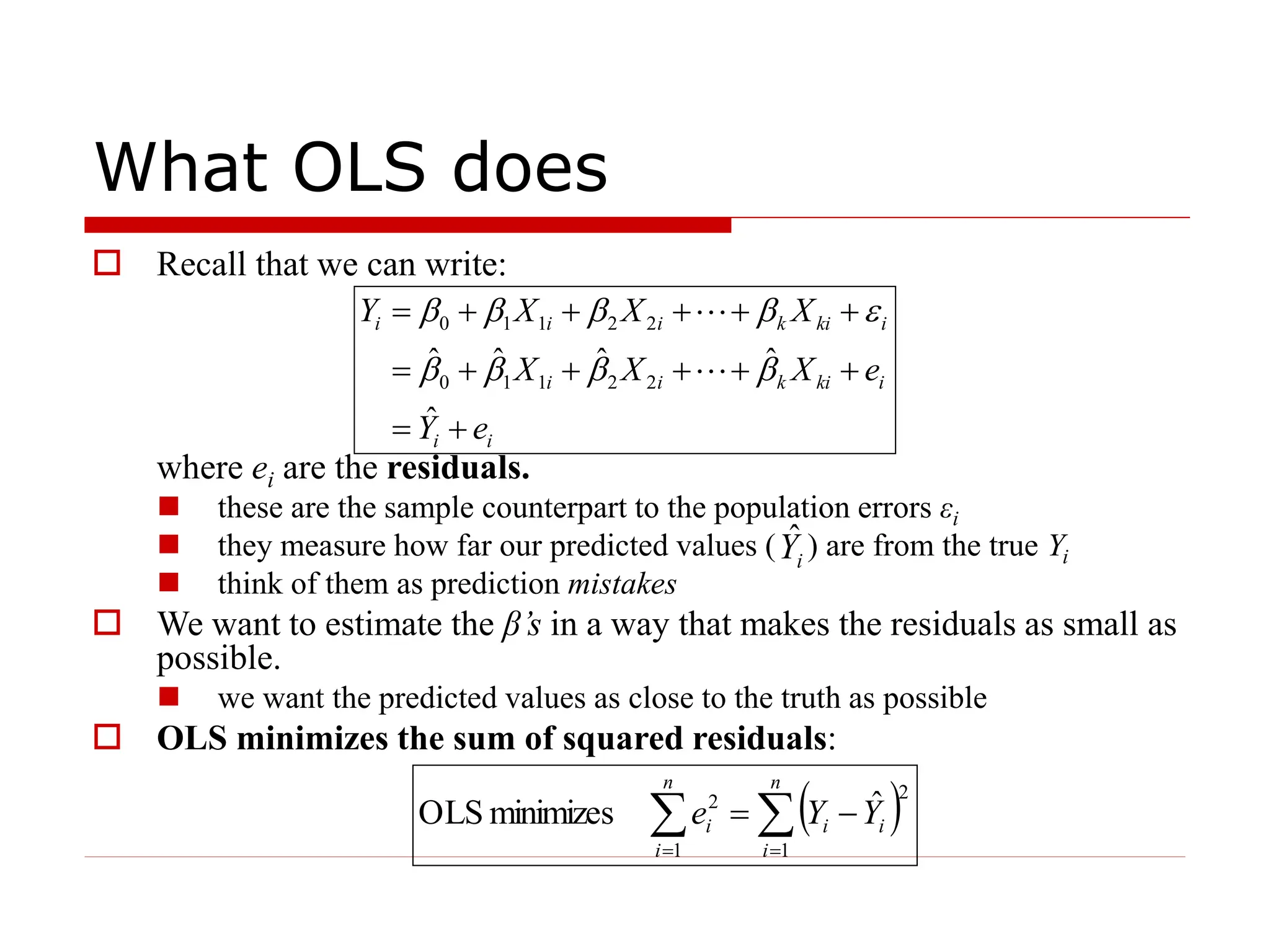
- Ordinary Least Squares (OLS) estimation is commonly used to estimate the coefficients in a linear regression model. OLS chooses coefficients that minimize the sum of squared residuals between predicted and actual values of the dependent variable. - OLS finds the coefficients that make the prediction errors as small as possible. It does this by minimizing the sum of squared errors between the predicted and actual y-values. 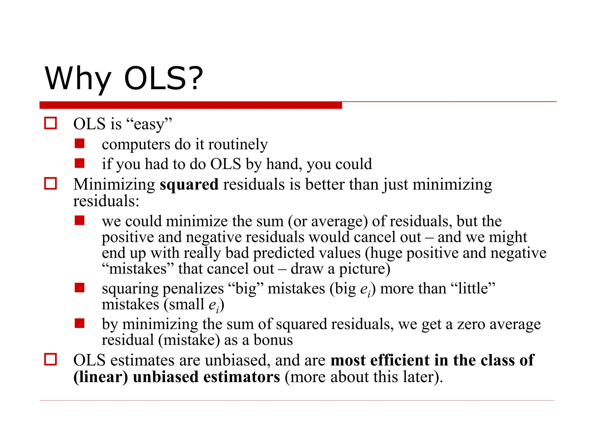- OLS provides unbiased estimates of the coefficients and produces estimates with the smallest possible variance, making it very widely used for linear regression analysis.

1. Ordinary Least Squares
Estimation
Simon Woodcock

2. From Last Day
 Recall our population regression function:
 Because the coefficients (β) and the errors (εi) are population quantities, we
don’t observe them.
 Sometimes our primary interest is the coefficients themselves
 βk measures the marginal effect of variable Xki on the dependent variable Yi.
 Sometimes we’re more interested in predicting Yi.
 if we have sample estimates of the coefficients, we can calculate predicted
values:
 In either case, we need a way to estimate the unknown β’s.
 That is, we need a way to compute from a sample of data
 It turns out there are lots of ways to estimate the β’s (compute ).
 By far the most common method is called ordinary least squares (OLS).
i
ki
k
i
i
i
i X
X
X
X
Y 




 





 
3
3
2
2
1
1
0
ki
k
i
i
i X
X
X
Y 


 ˆ
ˆ
ˆ
ˆ
ˆ
2
2
1
1
0 



 
s
'
ˆ

s
'
ˆ


3. What OLS does
 Recall that we can write:
where ei are the residuals.
 these are the sample counterpart to the population errors εi
 they measure how far our predicted values ( ) are from the true Yi
 think of them as prediction mistakes
 We want to estimate the β’s in a way that makes the residuals as small as
possible.
 we want the predicted values as close to the truth as possible
 OLS minimizes the sum of squared residuals:
i
i
i
ki
k
i
i
i
ki
k
i
i
i
e
Y
e
X
X
X
X
X
X
Y














ˆ
ˆ
ˆ
ˆ
ˆ
2
2
1
1
0
2
2
1
1
0











i
Y
ˆ
 
 
 


n
i
n
i
i
i
i Y
Y
e
1 1
2
2 ˆ
minimizes
OLS

4. Why OLS?
 OLS is “easy”
 computers do it routinely
 if you had to do OLS by hand, you could
 Minimizing squared residuals is better than just minimizing
residuals:
 we could minimize the sum (or average) of residuals, but the
positive and negative residuals would cancel out – and we might
end up with really bad predicted values (huge positive and negative
“mistakes” that cancel out – draw a picture)
 squaring penalizes “big” mistakes (big ei) more than “little”
mistakes (small ei)
 by minimizing the sum of squared residuals, we get a zero average
residual (mistake) as a bonus
 OLS estimates are unbiased, and are most efficient in the class of
(linear) unbiased estimators (more about this later).

5. How OLS works
 Suppose we have a linear regression model with one independent
variable:
 The OLS estimates of β0 and β1 are the values that minimize:
 you all know how to solve for the OLS estimates. We just differentiate this
expression with respect to β0 and β1, set the derivatives equal to zero, and
solve.
 The solutions to this minimization problem are (look familiar?):
i
i
i X
Y 

 

 1
0
   

  
 





n
i
i
i
n
i
n
i
i
i
i X
Y
Y
Y
e
1
2
1
0
1 1
2
2 ˆ
ˆ
ˆ 

  
 
X
Y
β
X
X
Y
Y
X
X
n
i
i
n
i
i
i
1
0
1
2
1
1
ˆ
ˆ
and
ˆ 
 










6. OLS in practice
 Knowing the summation formulas for OLS
estimates is useful for understanding how OLS
estimation works.
 once we add more than one independent variable,
these summation formulas become cumbersome
 In practice, we never do least squares calculations
by hand (that’s what computers are for)
 In fact, doing least squares regression in
EViews is a piece of cake – time for an
example.

7. An example
 Suppose we are interested in how an NHL hockey player’s salary varies
with the number of points they score.
 it’s natural to think variation in salary is related to variation in points scored
 our dependent variable (Yi) will be SALARY_USD
 our independent variable (Xi) will be POINTS
 After opening the EViews workfile, there are two ways to set up the
equation:
1. select SALARY_USD and then POINTS (the order is important), then
right-click one of the selected objects, and OPEN -> AS EQUATION
or
2. QUICK -> ESTIMATE EQUATION and then in the EQUATION
SPECIFICATION dialog box, type:
salary_usd points c
(the first variable in the list is the dependent variable, the remaining
variables are the independent variables including the intercept c)
 You’ll see a drop down box for the estimation METHOD, and notice that
least squares (LS) is the default. Click OK.
 It’s as easy as that. Your results should look like the next slide ...

8. Estimation Results

9. What the results mean
 The column labeled “Coefficient” gives the least squares estimates of the
regression coefficients.
 So our estimated model is:
USD_SALARY = 335602 + (41801.42)*POINTS
 That is, players who scored zero points earned $335,602 on average
 For each point scored, players were paid an additional $41,801 on average
 So the “average” 100-point player was paid $4,515,702
 The column labeled “Std. Error” gives the standard error (square root of the
sampling variance) of the regression coefficients
 the OLS estimates are functions of the sample data, and hence are RVs – more
on their sampling distribution later
 The column labeled “t-Statistic” is a test statistic for the null hypothesis that
the corresponding regression coefficient is zero (more about this later)
 The column labeled “Prob.” is the p-value associated with this test
 Ignore the rest for now
 Now let’s see if anything changes when we add a player’s age & years of
NHL experience to our model

10. Another Example

11. What’s Changed: The Intercept
 You’ll notice that the estimated coefficient on POINTS and the intercept
have changed.
 This is because they now measure different things.
 In our original model (without AGE and YEARS_EXP among the
independent variables), the intercept (c) measured the average
USD_SALARY when POINTS was zero ($335,602)
 That is, the intercept estimated E(USD_SALARY | POINTS=0)
 This quantity puts no restriction on the value of AGE and YEARS_EXP
 In the new model (including AGE and YEARS_EXP among the
independent variables), the intercept measures the average
USD_SALARY when POINTS, AGE, and YEARS_EXP are all zero
($419,897.8)
 That is, the new intercept estimates
E(USD_SALARY | POINTS = 0, AGE = 0, YEARS_EXP = 0)

12. What’s Changed: The Slope
 In our original model (excluding AGE and YEARS_EXP), the coefficient
on POINTS was an estimate of the marginal effect of POINTS on
USD_SALARY, i.e.,
 This quantity puts no restriction on the values of AGE and YEARS_EXP
(implicitly, we are allowing them to vary along with POINTS) – it’s a total
derivative
 In the new model (which includes AGE and YEARS_EXP), the coefficient
on POINTS measures the marginal effect of POINTS on USD_SALARY
holding AGE and YEARS_EXP constant, i.e.,
 That is, it’s a partial derivative
 The point: what your estimated regression coefficients measure
depends on what is (and isn’t) in your model!
42
41801
(POINTS)
Y)
(USD_SALAR
.
d
d

37
.
36603
(POINTS)
Y)
(USD_SALAR


