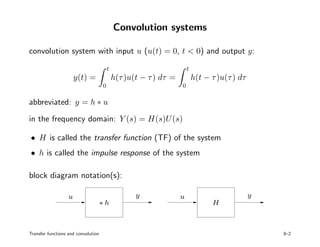
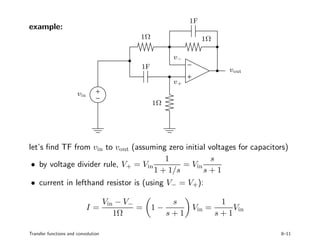
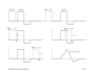
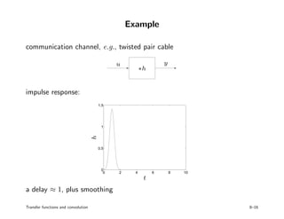
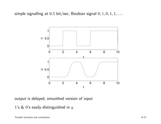
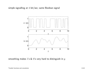
S. Boyd EE102
Lecture 8
Transfer functions and convolution
• convolution & transfer functions
• properties
• examples
• interpretation of convolution
• representation of linear time-invariant systems
8–1
Convolution systems
convolution system with input u (u(t) = 0, t < 0) and output y:
y(t) =
t
0
h(τ)u(t − τ) dτ =
t
0
h(t − τ)u(τ) dτ
abbreviated: y = h ∗ u
in the frequency domain: Y (s) = H(s)U(s)
• H is called the transfer function (TF) of the system
• h is called the impulse response of the system
block diagram notation(s):
PSfrag replacements
u y u y
∗ h H
Transfer functions and convolution 8–2
Properties
1. convolution systems are linear: for all signals u1, u2 and all α, β ∈ R,
h ∗ (αu1 + βu2) = α(h ∗ u1) + β(h ∗ u2)
2. convolution systems are causal: the output y(t) at time t depends only
on past inputs u(τ), 0 ≤ τ ≤ t
3. convolution systems are time-invariant: if we shift the input signal u
over T > 0, i.e., apply the input
u(t) =
0 t < T
u(t − T) t ≥ 0
to the system, the output is
y(t) =
0 t < T
y(t − T) t ≥ 0
in other words: convolution systems commute with delay
Transfer functions and convolution 8–3
4. composition of convolution systems corresponds to
• multiplication of transfer functions
• convolution of impulse responses
PSfrag replacements
u
u
composition
y
yA B
BA
ramifications:
• can manipulate block diagrams with transfer functions as if they were
simple gains
• convolution systems commute with each other
Transfer functions and convolution 8–4
Example: feedback connection
PSfrag replacements
u G y
in time domain, we have complicated integral equation
y(t) =
t
0
g(t − τ)(u(τ) − y(τ)) dτ
which is not easy to understand or solve . . .
in frequency domain, we have Y = G(U − Y ); solve for Y to get
Y (s) = H(s)U(s), H(s) =
G(s)
1 + G(s)
(as if G were a simple scaling system!)
Transfer functions and convolution 8–5
General examples
first order LCCODE: y + y = u, y(0) = 0
take Laplace transform to get
Y (s) =
1
s + 1
U(s)
transfer function is 1/(s + 1); impulse response is e−t
integrator: y(t) =
t
0
u(τ) dτ
transfer function is 1/s; impulse response is 1
delay: with T ≥ 0,
y(t) =
0 t < T
u(t − T) t ≥ T
impulse response is δ(t − T); transfer function is e−sT
Transfer functions and convolution 8–6
Vehicle suspension system
(simple model of) vehicle suspension system:
PSfrag replacements
u
y
m
k b
• input u is road height (along vehicle path); output y is vehicle height
• vehicle dynamics: my + by + ky = bu + ku
assuming y(0) = 0, y (0) = 0, (and u(0−) = 0),
(ms2
+ bs + k)Y = (bs + k)U
TF from road height to vehicle height is H(s) =
bs + k
ms2 + bs + k
Transfer functions and convolution 8–7
DC motor
PSfrag replacements
i θ
Jθ + bθ = ki
(J is rotational inertia of shaft & load; b is mechanical resistance of shaft
& load; k is motor constant)
assuming θ(0) = θ (0) = 0,
Js2
Θ(s) + bsΘ(s) = kI(s), Θ(s) =
k
Js2 + bs
I(s)
i.e., transfer function H from i to θ is
H(s) =
k
Js2 + bs
Transfer functions and convolution 8–8
Circuit examples
consider a circuit with linear elements, zero initial conditions for inductors
and capacitors,
• one independent source with value u
• y is a voltage or current somewhere in the circuit
then we have Y (s) = H(s)U(s)
example: RC circuit
PSfrag replacements
u y
R
C
RCy (t) + y(t) = u(t), Y (s) =
1
1 + sRC
U(s)
impulse response is L−1 1
1 + sRC
=
1
RC
e−t/RC
Transfer functions and convolution 8–9
to find H: write circuit equations in frequency domain:
• resistor: v(t) = Ri(t) becomes V (s) = RI(s)
• capacitor: i(t) = Cv (t) becomes I(s) = sCV (s)
• inductor: v(t) = Li (t) becomes V (s) = sLI(s)
in frequency domain, circuit equations become algebraic equations
Transfer functions and convolution 8–10
example:
PSfrag replacements
vin
vout
1Ω
1Ω
1Ω
1F
1F
v−
v+
let’s find TF from vin to vout (assuming zero initial voltages for capacitors)
• by voltage divider rule, V+ = Vin
1
1 + 1/s
= Vin
s
s + 1
• current in lefthand resistor is (using V− = V+):
I =
Vin − V−
1Ω
= 1 −
s
s + 1
Vin =
1
s + 1
Vin
Transfer functions and convolution 8–11
• I flows through 1F 1Ω, yielding voltage
Vin
1
s + 1
(1)(1/s)
1 + 1/s
= Vin
1
(s + 1)2
• finally we have Vout = V− − Vin
1
(s + 1)2
= Vin
s2
+ s − 1
(s + 1)2
so transfer function is
H(s) =
s2
+ s − 1
(s + 1)2
= 1 −
1
s + 1
−
1
(s + 1)2
impulse response is
h(t) = L−1
(H) = δ(t) − e−t
− te−t
we have
vout(t) = vin(t) −
t
0
(1 + τ)e−τ
vin(t − τ) dτ
Transfer functions and convolution 8–12
Interpretation of convolution
y(t) =
t
0
h(τ)u(t − τ) dτ
• y(t) is current output; u(t − τ) is what the input was τ seconds ago
• h(τ) shows how much current output depends on what input was τ
seconds ago
for example,
• h(21) big means current output depends quite a bit on what input was,
21sec ago
• if h(τ) is small for τ > 3, then y(t) depends mostly on what the input
has been over the last 3 seconds
• h(τ) → 0 as τ → ∞ means y(t) depends less and less on remote past
input
Transfer functions and convolution 8–13
Graphical interpretation
y(t) =
t
0
h(t − τ)u(τ) dτ
to find y(t):
• flip impulse response h(τ) backwards in time (yields h(−τ))
• drag to the right over t (yields h(t − τ))
• multiply pointwise by u (yields u(τ)h(t − τ))
• integrate over τ to get y(t)
Transfer functions and convolution 8–14
placements
h(τ) u(τ)u(τ) h(−τ)
h(t1 − τ) h(t2 − τ)
h(t3 − τ)
τ
τ
τ
τ
τ
τ
y = u ∗ h
t1 t2
t3
Transfer functions and convolution 8–15
Example
communication channel, e.g., twisted pair cable
PSfrag replacements
u y
∗h
impulse response:
0 2 4 6 8 10
0
0.5
1
1.5
PSfrag replacements
t
h
a delay ≈ 1, plus smoothing
Transfer functions and convolution 8–16
simple signalling at 0.5 bit/sec; Boolean signal 0, 1, 0, 1, 1, . . .
0 2 4 6 8 10
0
0.5
1
0 2 4 6 8 10
0
0.5
1
PSfrag replacements
t
t
uy
output is delayed, smoothed version of input
1’s & 0’s easily distinguished in y
Transfer functions and convolution 8–17
simple signalling at 4 bit/sec; same Boolean signal
0 2 4 6 8 10
0
0.5
1
0 2 4 6 8 10
0
0.5
1
PSfrag replacements
t
t
uy
smoothing makes 1’s & 0’s very hard to distinguish in y
Transfer functions and convolution 8–18
Linear time-invariant systems
consider a system A which is
• linear
• time-invariant (commutes with delays)
• causal (y(t) depends only on u(τ) for 0 ≤ τ ≤ t)
called a linear time-invariant (LTI) causal system
we have seen that any convolution system is LTI and causal; the converse
is also true: any LTI causal system can be represented by a convolution
system
convolution/transfer function representation gives universal description for
LTI causal systems
(precise statement & proof is not simple . . . )
Transfer functions and convolution 8–19

Tf

  • 1.
    S. Boyd EE102 Lecture8 Transfer functions and convolution • convolution & transfer functions • properties • examples • interpretation of convolution • representation of linear time-invariant systems 8–1
  • 2.
    Convolution systems convolution systemwith input u (u(t) = 0, t < 0) and output y: y(t) = t 0 h(τ)u(t − τ) dτ = t 0 h(t − τ)u(τ) dτ abbreviated: y = h ∗ u in the frequency domain: Y (s) = H(s)U(s) • H is called the transfer function (TF) of the system • h is called the impulse response of the system block diagram notation(s): PSfrag replacements u y u y ∗ h H Transfer functions and convolution 8–2
  • 3.
    Properties 1. convolution systemsare linear: for all signals u1, u2 and all α, β ∈ R, h ∗ (αu1 + βu2) = α(h ∗ u1) + β(h ∗ u2) 2. convolution systems are causal: the output y(t) at time t depends only on past inputs u(τ), 0 ≤ τ ≤ t 3. convolution systems are time-invariant: if we shift the input signal u over T > 0, i.e., apply the input u(t) = 0 t < T u(t − T) t ≥ 0 to the system, the output is y(t) = 0 t < T y(t − T) t ≥ 0 in other words: convolution systems commute with delay Transfer functions and convolution 8–3
  • 4.
    4. composition ofconvolution systems corresponds to • multiplication of transfer functions • convolution of impulse responses PSfrag replacements u u composition y yA B BA ramifications: • can manipulate block diagrams with transfer functions as if they were simple gains • convolution systems commute with each other Transfer functions and convolution 8–4
  • 5.
    Example: feedback connection PSfragreplacements u G y in time domain, we have complicated integral equation y(t) = t 0 g(t − τ)(u(τ) − y(τ)) dτ which is not easy to understand or solve . . . in frequency domain, we have Y = G(U − Y ); solve for Y to get Y (s) = H(s)U(s), H(s) = G(s) 1 + G(s) (as if G were a simple scaling system!) Transfer functions and convolution 8–5
  • 6.
    General examples first orderLCCODE: y + y = u, y(0) = 0 take Laplace transform to get Y (s) = 1 s + 1 U(s) transfer function is 1/(s + 1); impulse response is e−t integrator: y(t) = t 0 u(τ) dτ transfer function is 1/s; impulse response is 1 delay: with T ≥ 0, y(t) = 0 t < T u(t − T) t ≥ T impulse response is δ(t − T); transfer function is e−sT Transfer functions and convolution 8–6
  • 7.
    Vehicle suspension system (simplemodel of) vehicle suspension system: PSfrag replacements u y m k b • input u is road height (along vehicle path); output y is vehicle height • vehicle dynamics: my + by + ky = bu + ku assuming y(0) = 0, y (0) = 0, (and u(0−) = 0), (ms2 + bs + k)Y = (bs + k)U TF from road height to vehicle height is H(s) = bs + k ms2 + bs + k Transfer functions and convolution 8–7
  • 8.
    DC motor PSfrag replacements iθ Jθ + bθ = ki (J is rotational inertia of shaft & load; b is mechanical resistance of shaft & load; k is motor constant) assuming θ(0) = θ (0) = 0, Js2 Θ(s) + bsΘ(s) = kI(s), Θ(s) = k Js2 + bs I(s) i.e., transfer function H from i to θ is H(s) = k Js2 + bs Transfer functions and convolution 8–8
  • 9.
    Circuit examples consider acircuit with linear elements, zero initial conditions for inductors and capacitors, • one independent source with value u • y is a voltage or current somewhere in the circuit then we have Y (s) = H(s)U(s) example: RC circuit PSfrag replacements u y R C RCy (t) + y(t) = u(t), Y (s) = 1 1 + sRC U(s) impulse response is L−1 1 1 + sRC = 1 RC e−t/RC Transfer functions and convolution 8–9
  • 10.
    to find H:write circuit equations in frequency domain: • resistor: v(t) = Ri(t) becomes V (s) = RI(s) • capacitor: i(t) = Cv (t) becomes I(s) = sCV (s) • inductor: v(t) = Li (t) becomes V (s) = sLI(s) in frequency domain, circuit equations become algebraic equations Transfer functions and convolution 8–10
  • 11.
    example: PSfrag replacements vin vout 1Ω 1Ω 1Ω 1F 1F v− v+ let’s findTF from vin to vout (assuming zero initial voltages for capacitors) • by voltage divider rule, V+ = Vin 1 1 + 1/s = Vin s s + 1 • current in lefthand resistor is (using V− = V+): I = Vin − V− 1Ω = 1 − s s + 1 Vin = 1 s + 1 Vin Transfer functions and convolution 8–11
  • 12.
    • I flowsthrough 1F 1Ω, yielding voltage Vin 1 s + 1 (1)(1/s) 1 + 1/s = Vin 1 (s + 1)2 • finally we have Vout = V− − Vin 1 (s + 1)2 = Vin s2 + s − 1 (s + 1)2 so transfer function is H(s) = s2 + s − 1 (s + 1)2 = 1 − 1 s + 1 − 1 (s + 1)2 impulse response is h(t) = L−1 (H) = δ(t) − e−t − te−t we have vout(t) = vin(t) − t 0 (1 + τ)e−τ vin(t − τ) dτ Transfer functions and convolution 8–12
  • 13.
    Interpretation of convolution y(t)= t 0 h(τ)u(t − τ) dτ • y(t) is current output; u(t − τ) is what the input was τ seconds ago • h(τ) shows how much current output depends on what input was τ seconds ago for example, • h(21) big means current output depends quite a bit on what input was, 21sec ago • if h(τ) is small for τ > 3, then y(t) depends mostly on what the input has been over the last 3 seconds • h(τ) → 0 as τ → ∞ means y(t) depends less and less on remote past input Transfer functions and convolution 8–13
  • 14.
    Graphical interpretation y(t) = t 0 h(t− τ)u(τ) dτ to find y(t): • flip impulse response h(τ) backwards in time (yields h(−τ)) • drag to the right over t (yields h(t − τ)) • multiply pointwise by u (yields u(τ)h(t − τ)) • integrate over τ to get y(t) Transfer functions and convolution 8–14
  • 15.
    placements h(τ) u(τ)u(τ) h(−τ) h(t1− τ) h(t2 − τ) h(t3 − τ) τ τ τ τ τ τ y = u ∗ h t1 t2 t3 Transfer functions and convolution 8–15
  • 16.
    Example communication channel, e.g.,twisted pair cable PSfrag replacements u y ∗h impulse response: 0 2 4 6 8 10 0 0.5 1 1.5 PSfrag replacements t h a delay ≈ 1, plus smoothing Transfer functions and convolution 8–16
  • 17.
    simple signalling at0.5 bit/sec; Boolean signal 0, 1, 0, 1, 1, . . . 0 2 4 6 8 10 0 0.5 1 0 2 4 6 8 10 0 0.5 1 PSfrag replacements t t uy output is delayed, smoothed version of input 1’s & 0’s easily distinguished in y Transfer functions and convolution 8–17
  • 18.
    simple signalling at4 bit/sec; same Boolean signal 0 2 4 6 8 10 0 0.5 1 0 2 4 6 8 10 0 0.5 1 PSfrag replacements t t uy smoothing makes 1’s & 0’s very hard to distinguish in y Transfer functions and convolution 8–18
  • 19.
    Linear time-invariant systems considera system A which is • linear • time-invariant (commutes with delays) • causal (y(t) depends only on u(τ) for 0 ≤ τ ≤ t) called a linear time-invariant (LTI) causal system we have seen that any convolution system is LTI and causal; the converse is also true: any LTI causal system can be represented by a convolution system convolution/transfer function representation gives universal description for LTI causal systems (precise statement & proof is not simple . . . ) Transfer functions and convolution 8–19